Evaluation and Hydrological Simulation of CMADS and CFSR Reanalysis Datasets in the Qinghai-Tibet Plateau


1
State Key Laboratory of Cryospheric Science, Northwest Institute of Eco-Environment and Resources, Chinese Academy of Sciences, Lanzhou 730000, China
2
University of Chinese Academy of Sciences, Beijing 100049, China
3
Institute of International Rivers and Eco-Security, Yunnan University, Kunming 650500, China
*
Author to whom correspondence should be addressed.
Water 2018, 10(4), 513; https://doi.org/10.3390/w10040513
Submission received: 11 March 2018
/
Revised: 9 April 2018
/
Accepted: 10 April 2018
/
Published: 20 April 2018
(This article belongs to the Special Issue Application of the China Meteorological Assimilation Driving Datasets for the SWAT Model (CMADS) in East Asia)
Abstract
:Multisource reanalysis datasets provide an effective way to help us understand hydrological processes in inland alpine regions with sparsely distributed weather stations. The accuracy and quality of two widely used datasets, the China Meteorological Assimilation Driving Datasets to force the SWAT model (CMADS), and the Climate Forecast System Reanalysis (CFSR) in the Qinghai-Tibet Plateau (TP), were evaluated in this paper. The accuracy of daily precipitation, max/min temperature, relative humidity and wind speed from CMADS and CFSR are firstly evaluated by comparing them with results obtained from 131 meteorological stations in the TP. Statistical results show that most elements of CMADS are superior to those of CFSR. The average correlation coefficient (R) between the maximum temperature and the minimum temperature of CMADS and CFSR ranged from 0.93 to 0.97. The root mean square error (RMSE) for CMADS and CFSR ranged from 3.16 to 3.18 °C, and ranged from 5.19 °C to 8.14 °C respectively. The average R of precipitation, relative humidity, and wind speed for CMADS are 0.46; 0.88 and 0.64 respectively, while they are 0.43, 0.52, and 0.37 for CFSR. Gridded observation data is obtained using the professional interpolation software, ANUSPLIN. Meteorological elements from three gridded data have a similar overall distribution but have a different partial distribution. The Soil and Water Assessment Tool (SWAT) is used to simulate hydrological processes in the Yellow River Source Basin of the TP. The Nash Sutcliffe coefficients (NSE) of CMADS+SWAT in calibration and validation period are 0.78 and 0.68 for the monthly scale respectively, which are better than those of CFSR+SWAT and OBS+SWAT in the Yellow River Source Basin. The relationship between snowmelt and other variables is measured by GeoDetector. Air temperature, soil moisture, and soil temperature at 1.038 m has a greater influence on snowmelt than others.
1. Introduction
The Qinghai-Tibet Plateau (TP, 26°–40° N, 73°–104° E) is the largest and highest plateau in the world, with an average altitude higher than 4000 m over an area of about 2.5 million km2 [1,2]. Complex orographic and harsh weather conditions make it difficult to install and maintain synoptic stations in the TP. Almost all of the existing stations are located in the east and south of TP, and 70% of the stations are located below 4000 m. Scarcity and low elevation of the existing weather stations cannot accurately present the meteorological status of the TP. Likewise, scarcity and weak representation of meteorological data is fruitless for developing hydrological models [3,4]. Distributed models scientifically delineate water cycles in basin-scales, but also need high quality weather data as input [5]. Therefore, the poorly observed network is one of the reasons for the slowly progress of hydrological simulation and analysis in the basins of the TP.
Reanalysis datasets are based on remote sensing products and climate model outputs, and some are corrected by observed data and are an important surrogate for observations [6]. They will play a major role in the development of models [7], showing climate change trends, [8] un-gauged regions [9]. However, in view of uncertainties which exist in the process of data acquisition and assimilation, most studies are still predicated on the evaluation of reanalysis [10]. The accuracy of reanalysis is mainly assessed in one of the following two ways: (1) comparison of reanalysis with corresponding observed data [11,12]; (2) using reanalysis as input data to drive hydrological models and then comparing the hydrological features of model output with the observed [13,14].
The first way is always used over a large-scale, with a certain number of weather stations. Many statistic indexes are utilized to measure the quality of reanalysis datasets, such as: correlation coefficient (R), relative bias (BIAS), root mean square error (RMSE) et al. Evaluation of average temperature and precipitation from reanalysis are more frequently used than other meteorological variables. Wang et al. [15] compared two types of ERA-Interim datasets with gridded observation datasets. Results showed that after topographic correction, temperature distribution of reanalysis closely reproduces the temperature conditions of the TP, and that the increased trend is similar to observed data. Likewise, achievements of Gao et al. [16] showed that ERA-Interim temperature in the TP works well; R of temperature in the monthly scale ranges from 0.973 to 0.999 when compared with 75 stations’ data above 3000 m. Song et al. [17] compared precipitation from eight gridded datasets with station observations in Asian high mountains; the result indicated that gauge-based or multi-source datasets showed better performance, and that merged datasets are of potential use in modeling water cycles. You et al. [18] compared multisource datasets with gridded precipitation observations over the TP; most datasets can capture the precipitation distribution and identity varieties of mean monthly precipitation. Wang et al. [19] compared precipitation, temperature, radiation, wind speed and surface pressure from six multi-reanalysis products with observed data. Results indicate that different products have different abilities in calculating meteorological elements. For example; ERA-Interim performance is good with temperature, whereas the Global Land Data Assimilation Systems (GLDAS) shows the best performance with precipitation. In conclusion, reanalysis datasets can display the broad distribution of meteorological elements of the TP, but corrections using observed data are essential to minimize errors.
With long continuous time series and high spatial resolution, reanalysis datasets are suitable to create hydrological models, especially in regions that have few weather stations. High quality temporal and spatial resolution meteorological input data for distributed models largely determines the result of model output. Much research evaluates reanalysis at the watershed-scale by using hydrological models. Thomas et al. [20] evaluated ten satellite and reanalysis datasets in six, different sized watersheds in West Africa. Gilles et al. [21] analyzed the impact of combining different reanalysis and weather station data on the accuracy of discharge modeling in Canada and the USA. Both concluded that reanalysis datasets can be an alternative for observed data. Some reanalysis datasets do well in runoff simulation, and NSE are satisfactory, especially in the reanalysis datasets bias-corrected by weather station data. Kan et al. [22] evaluated “the Climate Prediction Center Morphing Technique (CMORPH)”, “Tropical Rain Measurement Mission Multi-satellite Precipitation Analysis (TRMM 3B42 V6)”, “China Meteorological Forcing Dataset (CMFD)” and “Asian Precipitation-Highly Resolved Observational Data Integration Towards Evaluation Of Water Resource (APHRODITE)” in the upper Yarkant River. Results indicate that datasets of distribution of precipitation from CMFD are more appropriate because they are consistent with the distribution of glaciers, and CMORPH based on satellite data, gets better results in forcing the Variable Infiltration Capacity (VIC) model. Guo et al. [23] compared two kind of multisource reanalysis data in hydrological simulation in the Lasa River Basin: the NSE is above 0.7 in the daily scale, and 0.8 in the monthly scale based on the HIMS model. Gao et al. [24] analyzed the application of CFSR, ERA-Interim in driving the VIC model in the Kash River Basins, and results indicate ERA-Interim is superior to CFSR. Hence, a set of reliable datasets can be a substitute for observed data in basins with sparsely distributed weather stations.
Previous studies, whether they use the first or the second method, always focus upon precipitation and average temperature. However, a complete set of data for distributed or semi-distributed hydrological models needs precipitation and average temperature, but also max/min temperatures, relative humidity, atmospheric pressure, wind speeds, solar radiation etc. For example, the SWAT model, as one of the most popular models, is extensively applied in runoff simulation and prediction, sediment transition etc. [25], and requires not only daily precipitation and temperature, but also relative humidity, atmospheric pressure, and wind speeds as input weather data, to obtain evapotranspiration [26]. Relative humidity, wind speed and max/min-temperatures also have great value in research. Relative humidity reflects the saturation of moisture in the atmosphere and has an impact on surface water, energy budgets, formation of aerosols, growth of plants and animals, etc. [27,28]. Wind speed depicts the movement of atmosphere and its influence affects other weather phenomena like precipitation, smog [29,30]. Maximum and minimum temperatures are more responsive to extreme weather events [31,32].
CMADS and CFSR, as two more complete datasets, contain several meteorological elements and are recommended by the SWAT official website (https://swat.tamu.edu/). CFSR has been widely used around the world. Dile et al. [33] and Abeyou et al. [34] used CFSR to drive three different hydrological models in the Blue Nile River Basin, and their results indicate that CFSR has the ability in forcing hydrological models; its simulation results were the same as, or better than, those forced by weather station data. In China, CFSR was used in the Bahe River Basin [35], Kaidu River Basin [36], Kash River Basins [24] etc. CMADS, built by Dr. Xianyong Meng from China Institute of Water Resources and Hydropower Research (IWHR), and bias-correction by observed data has been used in several basins including China’s Juntanghu watershed [37,38,39] and the Manas River Basin [40]; the results are satisfactory. However, comprehensive evaluation and application of these two datasets in the TP is scarce, especially CMADS. Thus, precipitation, max/min-temperatures, relative humidity and wind speed from CMADS and CFSR were evaluated using data from 131 weather stations in this paper. The Yellow River Source Basin was also selected for hydrological simulation and analysis.
2. Study Area
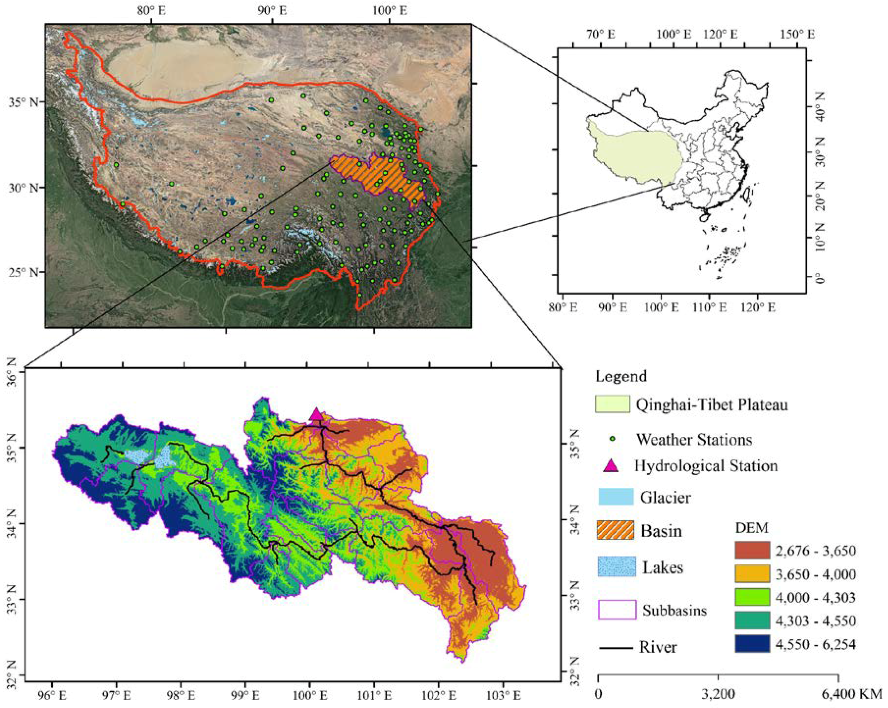
Located in south central Eurasia, affected by high elevation and far from the ocean, the TP forms a complex plateau climate system. The average annual temperature ranges from 20 °C in the southeast to −6 °C in the northwest, and precipitation declines from 2000 to 50 mm, correspondingly [41]. The TP is composed of a series of plateaus, mountains and valleys. The Yellow River Source Basin was selected to analyze the ability of two reanalysis in forcing hydrological models. The Yellow River Source Basin is located in the northeastern part of the TP (Figure 1), and refers to the basin above the Tangnaihai hydrological station (100°09′ E,35°30′ N, 2546 m) [42]. The catchment area is about 122 thousand square kilometers and the elevation ranges from 2676 to 6254 m (Figure 1). Permafrost is widely distributed within the Yellow River Source Basin, and most of it is seasonally frozen. The Yellow River Source Basin is rich in water resources and there are a large number of plateau lakes and wetlands. The Zaling and Erling lakes are the highest freshwater lakes in China [43].
3. Data and Methods
3.1. Data
The China Meteorological Assimilation Driving Datasets for the SWAT model version 1.0 (CMADS V1.0) was developed by Dr. Xianyong Meng using STMAS assimilation techniques [44]. Temperature, atmospheric pressure, specific humidity and wind speed of CMADS is based on The National Center for Environmental Prediction Global Forecast System (NECP/GFS), and is corrected by observed data. The background field for precipitation is CMORPH, and this is adjusted by observed precipitation data [44]. CMADS V1.0 provides: daily maximum/average/minimum temperatures, cumulative 24 h-precipitation, average solar radiation, air pressure, relative humidity, and average wind speed from 2008 to 2016. Ten layers of soil temperature from CMADS-ST are also used in this paper [45,46]. The depth from the first to the tenth are 0.007 m, 0.028 m, 0.062 m, 0.119 m, 0.212 m, 0.366 m, 0.62 m, 1.038 m, 1.727 m and 2.865 m. Climate and soil temperature data of CMADS can be downloaded CMADS official website (http://www.cmads.org/).
The Climate Forecast System Reanalysis datasets (CFSR) is developed by The National Center for Environmental Prediction (NCEP) and is derived from the Global Forecast System [47]. With high spatial resolution, reliability and long time series, CFSR is widely used in climate analysis and hydrological simulation. The SWAT official website provides data from a 36-year period (from 1979 to 2014) in the format requested by the SWAT model, with elements including: precipitation, max/min temperatures, relative humidity, wind speed and solar radiation [33]. For comparison purposes, we selected the period from 2008 to 2014; the CFSR dataset was freely accessible from the SWAT official website (https://globalweather.tamu.edu/).
We also collected measured data from 131 weather stations (Figure 1); meteorological elements included: mean/max/min temperatures, precipitation, wind speed, and relative humidity in daily scale, provided by the China Meteorological Administration Meteorological Data Center. Among the 131 weather stations, elevation of 9 stations are less than 2000 m, 42 stations are between 2000 and 3000 m, 55 stations range from 3000 to 4000 m, and 25 stations are above 4000 m, with highest at an altitude of 4800 m. Seventy four percent of sites were at an elevation of between 2000 and 4000 m.
Geographical and hydrological data includes: DEM (digital elevation model), soil, land cover, the 90 m DEM was downloaded from CGIAR-CSI (http://srtm.csi.cgiar.org/). Soil and land use data was provided by the Cold and Arid Regions Sciences Data Center at Lanzhou (http://westdc.westgis.ac.cn/).
3.2. Hydrological Models
SWAT was developed by the US Department of Agriculture in the 1990s and plays an important role in runoff simulation, sediment movement, and non-point source modeling [48]. According to elevation, a watershed will be divided into several sub-basins which will be further divided into hydrological response units (HRUs) based on land use, soil type and slope. Water balance will be calculated in each HRU. Soil Convention Service (SCS) runoff curve and Penman-Monteith methods are used to model surface runoff process and evapotranspiration. Precipitation will be divided into rain or snow, according to critical temperature. Snowfall is stored as snow on the surface, and the process of addition (), ablation () and sublimation will be calculated by the snow mass conservation Equation (1). Degree day method is used to simulate snow melt (), the snow temperature (), daily maximum temperature of the basin () and snowmelt threshold temperature () combined with snow cover area () and degree-day factor (). These parameters pertain to snowmelt, and their relationship is Equation (2). Lakes and reservoirs belong to the river network water cycle calculation. Wetland belongs to corresponding sub-basins, and the change is also based on the corresponding water balance equation. Therefore, SWAT has the ability to simulate the complicated hydrological process of the Yellow River Source Basin, which is a snow dominated watershed with wetland, lakes etc.
3.3. Spatial Analysis Methods
Observed meteorological data from 131 weather stations are used to interpolate though ANUSPLIN, which is a professional interpolation software based on the thin plate smooth spline technique. Wahba proposed the thin plate smoothing spline surface fitting technique in 1979; the theoretical model formula is as follows,
is a dependent variable, is independent variable, f is unknown smooth function, is independent covariate, b is coefficient and is random error.
Bates, Eblen, Hutchinson et al. updated this spatial interpolation method and eventually formed ANUSPLIN [49]. ANUSPLIN is convenient and has been widely used in Australia, Europe, the United States etc. [50]; more detailed information about each module is described by Liu et al. [51].
GeoDetector is an effective way to measure spatially stratified heterogeneity of variables, and to test the connection between variables according to the consistency of their spatial distributions [52]. It is widely used in the field of health to detect the correlation of distribution of disease incidence and their impact factors. However, Zhao et al. [53] use this model to analysis the impacts of terrestrial environmental factors on precipitation variation over the Beibu Gulf Economic Zone in Coastal Southwest China. Foroogh et al. [54] used this method to analyze the relationship between air temperature and land use, elevation, latitude et al. Therefore, we use this detector model for quantitative analysis of the relationship between snow melt and related factors, like soil temperature, soil humidity, or topographic parameters. The parameter to measure the degree of correlation between variables is q-stastic, and the formula is as follows,
stands for the variance of Y; N is the number of units of Y; Y is composed of L strata (h = 1, 2, …, L). It should be noted that q ϵ [0,1], and q = 0 means there is no association between Y and X; q = 1 indicates Y is completely determined by X.
3.4. Evaluation Index
The correlation coefficient (R), relative bias (BIAS), root mean square error (RMSE) and ratio of standard deviation (σ/σobs) are used to measure the accuracy of reanalysis datasets compared to observed data in both daily and monthly scale. R is Pearson correlation coefficient (R) and its square is coefficient of determination (R2). They are used to measure the correlation between variables. The range of R and R2 is [0,1]. If R = 0, there is no correlation between two variables. If R = 1, the two variables are linearly related. BIAS and RMSE are used to measure the deviation between variables; ranges are [−∞,+∞] and [0,+∞] respectively. σ/σobs is used to measure the simulated value compared to observed data.
Nash-Sutcliffe Efficiency (NSE) and the coefficient of determination (R2) are used to evaluate the simulation effect of hydrological models on runoff, the range is (−∞,1). 0.75 < NSE ≤ 1 means that the simulation results are excellent, 0.65 < NSE ≤ 0.75 means the simulation results are good. 0.5 < NSE ≤ 0.65 means the simulation results are acceptable. When NSE < 0.5, the simulation filed and the results is unacceptable [55]. NSE and R2 are calculated as follows,
4. Results
4.1. Comparison of CMADS and CFSR with Observation Data
Precipitation is affected by multi-factors and has large spatial heterogeneity in alpine regions, which is very difficult to capture accurately (Figure 2). Mean R of CMADS precipitation is within 0.16–0.66, with an average value of 0.46; Sixty-four percent of stations drop to 0.4–0.6 (Table 1). Range of BIAS is from −0.64 to 3.76, with an average value of 0.08, among which 56% weather stations have a positive value, 44% have a negative bias, and three stations have abnormal BIAS values beyond 2. RMSE ranges from 0.54 to 6.78 mm, and 80% stations are located in the 3–5 mm range with an average value of 3.77 mm. σ/σobs stands for the ratio of deviation used to measure the dissociation of two time series. σ/σobs of CMADS precipitation is within 0.28–2.12, with an average value of 1.07. Among the 131 stations, just one station is beyond 2, meaning that the degree of deviation is twice that of the observed data in this station. For CFSR, the evaluation results are still not grounds for optimism. Mean R of precipitation is in the range of 0.13–0.6, with a mean value of 0.43, approaching the result of CMADS; Sixty-five percent of stations are within 0.4–0.5 (Figure 2). BIAS shows that 77% stations overestimate precipitation, and one station presents unusually beyond 10. RMSE of CFSR precipitation ranges between 1.38 and 13.67 mm, with an average value of 4.5 mm; 22% stations are greater than 5 mm. Compared with observed data, σ/σobs of 63% of stations is larger than observations, and 9 stations are double. Precipitation of CMADS uses CMORPH as the background field and assimilates more than 30,000 mobile observation stations in China. CMORPH is derived from low orbiter satellite microwave observations, whose features are transported via spatial propagation information that is obtained entirely from geostationary satellite IR data. However, precipitation observed by satellites always underestimate light rainfall events, and tend to fail over snow- and ice-coved surfaces [56]; these system biases results in underestimation of precipitation provided by CMADS. CFSR is derived from the global forecast system and this dataset always overestimates precipitation in northwest China, which have been obtained in many studies [24,36,57,58].
Evaluation of results of max/min temperatures improved significantly compared to precipitation: R of CMADS max/min-temperatures are close to 1 and CFSR is within 0.78–0.98 (Table 1). However, CMADS underrates max/min-temperatures since the BIAS of max-temperature of 94% stations is less than zero and the corresponding value of min-temperature is 52%. Meanwhile, all 131 BIAS of CFSR max-temperatures have a cold value with the mean value of −0.56. This result improves in min-temperature, although 60% stations have a cold value. The RMSE is not optimal; this is also the case with Gao et al. [16], where RMSE is within 0.78–16.9 °C of CMADS maximum temperature and 1.4–10 °C of min-temperature, and the range for CFSR maximum and minimum temperature are 2.4–16 °C and 2.2–12.8 °C respectively. Two stations of CMADS maximum temperature have RMSE value 16.9 °C and 14.2 °C, and others lower than 10 °C. Forty-one stations have a RMSE of max-temperature of CFSR higher than 10 °C. The σ/σobs, of the maximum minimum temperature performs better and most stations of CMADS and CFSR are close to 1.
Evaluation results of relative humidity still have a gap between CMADS and CFSR (Figure 2). R of CMADS relative humidity is within 0.66–0.95, with an average value of 0.88, and 86% stations record above 0.8. Average value of BIAS is 0.01, and 62% have a negative value. RMSE is in the range of 3.99–22.4%, with a mean value of 8.9%, and 68% stations are within 10%. σ/σobs is within 0.7–1.33, with average value 1.09. R of CFSR relative humidity is within 0.13–0.79 with an average value of 0.51; average BIAS is 0.22. RMSE is within the range of 11.9–44.7%, and the average value is 20.63%. The wind speed of CFSR is worse, with an average R of 0.36; BIAS is 0.83, the average RMSE is 1.93 m/s, and average σ/σobs is 1.5 times that of observation. Thirty-two percent stations have a BIAS greater than 1, and 7 stations have a negative value; 40% show RMSE over 2 m/s. As for CMADS, BIAS of 91% stations has a negative value, which indicates that CMADS underestimates wind speed in the TP. The average value of R, BIAS and RMSE improved significantly compared with CFSR but a small number of stations still underperformed. Temperature, humidity and wind speed of CMADS are based on NCEP/GFS; they assimilate 2421 national automatic stations and 39,439 regional climate stations, so the results are an improvement compared to CFSR. Thus, observed climate data plays a significant role in the process of developing a high-quality reanalysis dataset.
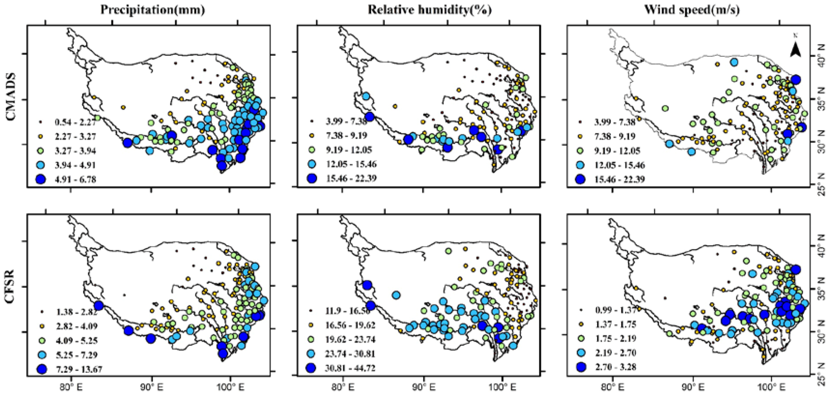
As is shown in Figure 3, the RMSE distribution of precipitation of CMADS decreases from southeast to northwest, which can be divided into four grades. The first gradient is the worst: RMSE ranges from 4.91 to 6.78 mm. All of these stations are located in the southeastern margin of the TP. Because of the complex orographic features and effects of the Pacific and Indian Ocean monsoons, this region’s precipitation exhibits large spatial heterogeneity. The second gradient surrounds the first gradient, mainly in the eastern and southern parts of the TP, and presents a RMSE range from 3.27 to 4.91 mm. The remaining stations are mainly located in the Qaidam Basin, which is flat and has a relatively stable weather pattern. This phenomenon is also reflected in the precipitation in the CFSR, which further corroborates the difficulty in describing precipitation in complex orographic regions. The abnormal values of relative humidity from both CMADS and CFSR are mainly located in the south of the TP. In the case of wind speed, three stations with large RMSE values are located in the east of the TP; this level of CFSR is mainly located in the south and east of the TP.
4.2. Distribution of Observed Data, CMADS and CFSR
We use ANUSPLIN to obtain gridded distribution of meteorological elements including precipitation, max/min temperatures, relative humidity and wind speed based on 131 observation stations with a spatial resolution of 0.3° (which approaches the resolution of CMADS V1.0 (1/3°) and CFSR (0.313°)). The distribution diagram displays the annual average values from 2008 to 2013.
Precipitation can be divided into three regions: abundant regions, relative rainy areas and arid regions (Figure 4). In the southeast margin of the TP, water vapor from Pacific and Indian Ocean brings abundant rainfall, so these are called abundant regions. Precipitation in this region is over 800 mm and, in some regions, greater than 1200 mm, as is shown by OBS (stands for ANUSPLIN interpolation results hereinafter). Precipitation distribution of CMADS in this region is not as high as OBS; some areas show precipitation within 800–1200 mm, others less than 800 mm, and a fraction show higher than 1200 mm. However, the precipitation of CFSR has abnormal characteristics: some regions show over 3000 mm, and individual sites even show over 10,000 mm. In addition, the annual average precipitation of CFSR in the southeast margin of the TP shows over 1200 mm. The second region is a relatively rainy area, that is, mainly around abundant regions and gradually decreases to the northwest. This is due to the increase in elevation, distance from the ocean, and a decrease in the presence of water vapor. This region shows a similarity between OBS and CMADS: precipitation is within 400–800 mm. The vast northwest is basically an arid region and precipitation is below 400 mm. Although precipitation of CFSR in this region still overestimated, it displays an obviously increasing trend from low altitudes to high mountains. This is important since precipitation in high mountainous areas occupies a vital status in runoff. In general, CMADS overestimated the amount of precipitation and CFSR widely overestimated it, compared with OBS.
Distribution of max/min-temperatures from OBS, CMADS and CFSR are more consistent when compared with precipitation (Figure 4). Factors which influence temperature are mainly (a) elevation, and (b) latitude. In the east of the TP, temperature increases from north to south with the corresponding decrease of latitude. Likewise, temperature decreases from east to west with elevation increase at the same latitude. In the southeast margin of the TP with low latitude and elevation, max/min-temperatures are high, and in the north-west high mountains, the opposite is true. CFSR underestimates maximum temperature in the south and east of the TP. Annual average Max-temperatures of OBS and CMADS mainly lie between 7 and 14 °C in the east and south of the TP, but in corresponding regions of CFSR records, they obviously go down.
Relative humidity is primarily affected by precipitation, and the distribution is consistent with precipitation (Figure 4). Relative humidity of CFSR is higher than in the observed data and CMADS in most part of the TP. For example, relative humidity of gridded observation and CMADS is within 30–40% in the south-central TP, but CFSR shows that it is within 40–60% in this region. In the hinterland, relative humidity of gridded observation and CMADS is within 30–40%, and the range of CFSR is 40–60%. Wind speed from gridded observation, CMADS and CFSR also show wide differences. Gridded observation reveals that annual average wind speed is in excess of 5 m/s in the northwest, but CMADS and CFSR do not show this characteristic, and the annual average wind speed is below 5 m/s. In the south east of the TP, wind speed of CFSR is overestimated at within 2–4 m/s, compared to 1–3 m/s, 1–2 m/s of gridded observation and CMADS respectively.
The TP is divided into three parts including: Tibet (Ι), Qinghai Provence (ΙΙ) and the remaining regions include parts of Gansu Provence, Sichuan Provence and Yunnan Provence (ΙΙΙ). Precipitation of CMADS is very close to observed data, but CFSR overestimates in all three regions (Figure 5). CMADS and CFSR underestimate maximum and minimum temperatures in most regions; only the comparison result of the minimum temperature of Qinghai Provence is satisfactory, and CFSR is substantially undervalued. Relative humidity and wind speed of CMADS and CFSR left little room for optimism: CFSR overestimates relative humidity in January to April and November to December in Qinghai Provence and each month is overvalued in Tibet and other regions. CMADS is consistent with observed data, except for a little overestimation in April to August in Tibet. Wind speed of CFSR still overestimated heavily in all three basins. Wind speed calculation of CMADS is more satisfactory in Tibet, but it underestimates in Qinghai and other regions. CMADS and CFSR calculate greater wind speed in winter and spring in comparison with summer and autumn, and this seasonal distribution is similar to the observed, gridded data (Figure 4).
4.3. Runoff Simulation in the Yellow River Source Basin
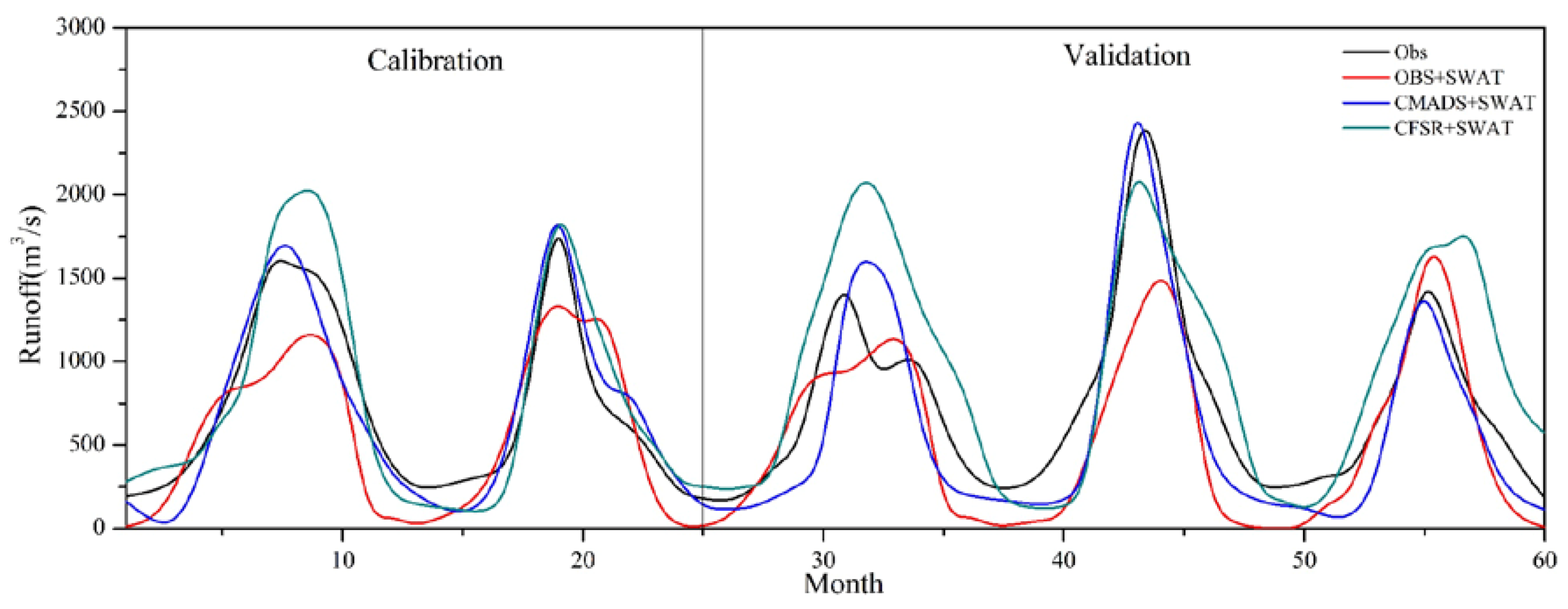
DEM is used in watershed delineation to generate stream networks and divide sub-basins; 25 sub-basins are divided in the Yellow River Source Basins. 2455 HRUs are generated by land use, soil and slope. Eleven observed stations, 107 CMADS grid, and 118 CFSR grid points are used to force SWAT in the Yellow River Source Basin. A weather generator which comes from the SWAT model is used to make up for the factors which are lacking from observed data. CMADS and CFSR provide all climate input data. Twelve sensitive parameters are selected to be calibrated. SWAT forced by CMADS (CMADS+SWAT) and CFSR (CFSR+SWAT) are better than observed data (OBS+SWAT) overall (Table 2 and Figure 6). In the monthly scale, NSE for CMADS+SWAT and CFSR+SWAT range from 0.42 to 0.68, which are improvements compared to OBS+SWAT. OBS+SWAT underestimate runoff: the NSE is −0.8 and −0.72 in calibration and validation over the period of a monthly scale. CFSR+SWAT overestimate runoff in most years and seriously overestimated the summer runoff in 2009, 2011 and 2013. NSE of CFSR+SWAT is 0.59 and 0.42 in calibration and validation over the period of a monthly scale. CMADS+SWAT do well in forcing the hydrological model and the simulation results are better, NSE of CMADS+SWAT is 0.68 to 0.58 in the monthly scale. In the daily scale, simulation results are not as good as in the monthly scale for all three datasets, but NSE of CMADS+SWAT is still above 0.5 (Table 2, Figure 7).
Different results of runoff simulation are mainly caused by the different climate forcing data. The SWAT output results show that annual average precipitation of CMADS is 560.1 mm in 2009–2013, and the corresponding value of OBS and CFSR are 536.5 mm, 815.4 mm respectively. This is consistent with the evaluation results. Precipitation of CFSR is overestimated in the TP (Table 1, Figure 2). The different amounts of precipitation result in the deviation simulation of runoff and streamflow of OBS+SWAT, CMADS+SWAT and CFSR+SWAT and are 171.9 mm, 203.4 mm, 284.7 mm respectively. However, evapotranspiration CMADS+SWAT and CFSR+SWAT is 314.8 mm, 526.4 mm. The difference between humidity, wind speed and max/min temperatures between CMADS and CFSR is the main reason for the deviation, according to Penman-Monteith.
4.4. Analysis of Snowmelt and Related variables
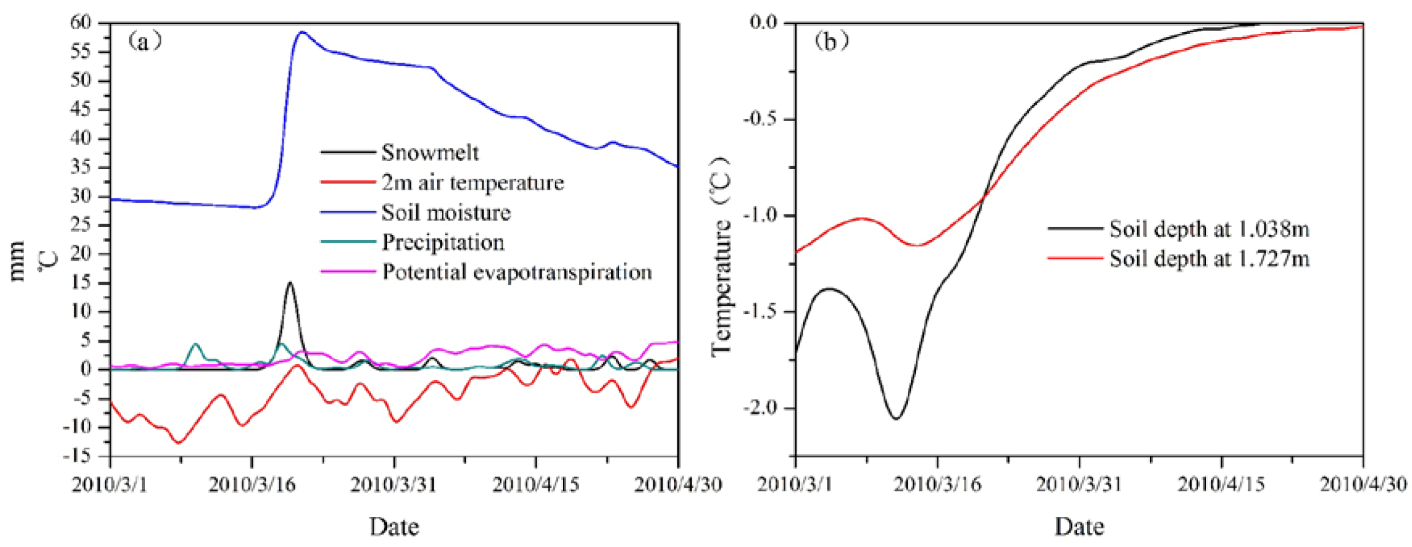
The hydrological process of CMADS+SWAT in March and April 2010 is used to find the relationship between snowmelt (Y) and other variables (X), including: precipitation, 2 m air temperature, solar radiation, soil relative humidity, potential evapotranspiration and soil temperature in different depths. q-statistic measures the association between Y and X variables, both linearly or nonlinearly. X are explanatory variables of Y, and the higher the q-statistic, the more contact between Y and X. Results of q value show that 2 m temperature and soil temperature at a depth of 1.038 m have greater effect on snowmelt; q-statistic values are 0.72 and 0.75 respectively. This is followed by soil relative humidity and soil temperature at depth of ST2, ST3, and ST9 (Table 3). Different q-statistics of different soil layer results from the complicated soil hydrothermal process during the snowmelt period [59]. Shallow soil temperatures are mainly affected by air temperature and have a high correlation with snowmelt results in q-statistics (which are high in ST2 and ST3 (Table 3)). Deep soil temperatures are protected by upper soil layers and have a smaller change. However, when the snow and frozen layers start to melt, this recharges the deeper layers and so the temperature will increase. Therefore, q-statistic of ST8 and ST9 is high.
The eighth sub-basin has a large amount of snowmelt and is selected for further analysis. Snowmelt increased significantly after March 16, accompanied by a rapid increase in soil moisture (Figure 8a). This process is caused by the increase of temperature. 2 m air temperature increased significantly around 16 March, and two depths soil temperature also show the same clear increase trend (Figure 8b). The change of snowmelt is stable before snowmelt, and soil moisture increased significantly as the snowmelt process occurs. Soil moisture supplementation by the melt of snow and frozen soil, and the large area of wetlands make this process more obvious. After snowmelt, evaporation rates increased and more soil water is evaporated. Deep soil temperature is less affected by air temperature, as shown in Figure 8. Before snowmelt, air temperature and soil temperature rises fluctuate, but as air temperature rises, there is an obvious increase in snowmelt and soil temperature.
5. Conclusions
Reanalysis datasets are an important alternative to observed data, especially for regions with few weather stations. They can provide several meteorological factors with higher-resolution data, which is profitable for hydrological simulation. However, various reanalysis datasets still have differences in sources, bias-corrected methods, resolution and temporal coverage et al. CMADS and CFSR are evaluated in this paper and the results show that bias-correction by observed weather data is important for reanalysis. CMADS assimilates nearly 40,000 regional automatic stations under China’s 2421 National Automatic and Business Assessment Centers, so that data accuracy is considerably improved. A complete set of data should contain as many climate elements as possible. Accuracy of relative humidity, wind speed, solar radiation etc. should receive more attention, not only due to their meteorological significance, but because they are also important to hydrological, ecological and erosion research etc. Evaluation results of CMADS and CFSR indicate that relative humidity and wind speed still have room for improvement (Table 1, Figure 2 and Figure 5). Besides, long-term series are more representative. CMADS just covers 9 years, compared to 35 years of CFSR, and is therefore too short. In overview, with good manifestation in meteorological elements and forcing hydrological models, it is hoped that authors expand the time series so as to provide convenience in assessing hydrological changes in a long-term context.
In this paper, precipitation, max/min temperatures, relative humidity and wind speed from CMADS and CFSR are evaluated. Discrepancies between these two datasets are fully demonstrated and main results are displayed as follows:
Compared with 131 metrological stations, daily precipitation is more difficult to simulate accurately. The average R for CMADS precipitation is 0.46, which is similar to CFSR (R = 0.43). R of CMADS and the CFSR max/min-temperatures is better, and the range is within 0.93–0.98. CMADS and CFSR both underestimate max/min-temperatures and average BIAS is cold. The average RMSE of max/min-temperatures is within 2.99–8.22 °C. Deviation of CMADS and CFSR temperature time series is close to observed data. Relative humidity and wind speed for CMADS is superior to those of CFSR according to various indexes.
The professional interpolation software ANUSPLIN is used to obtain the spatial distribution of annual average precipitation, max/min-temperatures, relative humidity and wind speed, based on the data from weather stations. Distribution of the three kinds of data is generally similar, but the local differences are more obvious. Precipitation of CFSR is overestimated in the whole TP, and unusually large values appeared in the southeast. Precipitation of CMADS is similar with observed data in distribution and in amount. As for the maximum and minimum temperatures, all three datasets have better consistency. Distribution of relative humidity of observed data shows that it is moister in the southeast and drier in the west, and this is different to what CMADS and CFSR present. A difference of distribution of wind speed is obvious in the northwest between observation and reanalysis.
CMADS has unique advantages in hydrological simulations compared with observed data and CFSR. Runoff simulations have achieved satisfactory results in the Yellow River Source Basin. NSE of CMADS+SWAT is 0.78 and 0.68 in calibration and validation, NSE of CFSR+SWAT is 0.69 and 0.52 in the Yellow River Source Basin and OBS+SWAT is unsatisfactory (NSE < 0). Obvious snow melting processes appeared in March and the temperature and soil moisture increased significantly around this time period. There are only eleven weather stations located in the Yellow River Source Basin, and these are located in the lower elevation areas of the eastern region, which means they are not representative. It is therefore difficult to achieve satisfactory simulation results only through adjustment of parameters in SWAT. Simulation results of runoff in the watershed are improved by two reanalysis datasets, due to their high resolution and quality, though CFSR overestimates precipitation in the Yellow River Source Basin, and results in excessive runoff. 2 m air temperature, soil moisture and 1.038 m depth soil temperature contribute more to snowmelt as shown, when measured by GeoDetector. Climate forcing data is important, deviation of precipitation (Table 1, Figure 2) results in the different amounts of runoff (Figure 6), and the temperature, humidity and wind speed, etc. also play an important role in calculating evapotranspiration. Evaluation of various reanalyses before forcing hydrological models is essential.
Acknowledgments
This work was financially supported by the National Natural Science Foundation of China (Grant nos. 41671066 & 41730751 & 41401084) and KJF-STS-ZDTP-015 & SKLCS-ZZ-2017.
Author Contributions
Donghui Shangguan, Shiyin Liu and Yongjian Ding conceived and designed the experiments; Jun Liu performed the experiments and wrote the paper.
Conflicts of Interest
The authors declare no conflict of interest.
References
- Qiu, J. The Third Pole. Nature 2008, 454, 393–396. [Google Scholar] [CrossRef] [PubMed]
- Zhang, Q.; Kong, D.; Shi, P.; Singh, V.P.; Sun, P. Vegetation phenology on the Qinghai-Tibetan Plateau and its response to climate change (1982–2013). Agric. For. Meteorol. 2018, 248, 408–417. [Google Scholar] [CrossRef]
- Zhou, J.; Pomeroy, J.W.; Zhang, W.; Cheng, G.; Wang, G.; Chen, C. Simulating cold regions hydrological processes using a modular model in the west of China. J. Hydrol. 2014, 509, 13–24. [Google Scholar] [CrossRef]
- Silberstein, R.P. Hydrological models are so good, do we still need data? Environ. Model. Softw. 2006, 21, 1340–1352. [Google Scholar] [CrossRef]
- Sun, W.; Ishidaira, H.; Bastola, S.; Yu, J. Estimating daily time series of streamflow using hydrological model calibrated based on satellite observations of river water surface width: Toward real world applications. Environ. Res. 2015, 139, 36–45. [Google Scholar] [CrossRef] [PubMed]
- Ma, Y.; Yang, Y.; Han, Z.; Tang, G.; Maguire, L.; Chu, Z.; Hong, Y. Comprehensive evaluation of Ensemble Multi-Satellite Precipitation Dataset using the Dynamic Bayesian Model Averaging scheme over the Tibetan plateau. J. Hydrol. 2018, 556, 634–644. [Google Scholar] [CrossRef]
- Huang, D.; Gao, S. Impact of different reanalysis data on WRF dynamical downscaling over China. Atmos. Res. 2018, 200, 25–35. [Google Scholar] [CrossRef]
- Agutu, N.O.; Awange, J.L.; Zerihun, A.; Ndehedehe, C.E.; Kuhn, M.; Fukuda, Y. Assessing multi-satellite remote sensing, reanalysis, and land surface models’ products in characterizing agricultural drought in East Africa. Remote Sens. Environ. 2017, 194, 287–302. [Google Scholar] [CrossRef]
- Moalafhi, D.B.; Sharma, A.; Evans, J.P. Reconstructing hydro-climatological data using dynamical downscaling of reanalysis products in data-sparse regions—Application to the Limpopo catchment in southern Africa. J. Hydrol. Reg. Stud. 2017, 12, 378–395. [Google Scholar] [CrossRef]
- Stopa, J.E.; Cheung, K.F. Intercomparison of wind and wave data from the ECMWF Reanalysis Interim and the NCEP Climate Forecast System Reanalysis. Ocean Model. 2014, 75, 65–83. [Google Scholar] [CrossRef]
- Sharp, E.; Dodds, P.; Barrett, M.; Spataru, C. Evaluating the accuracy of CFSR reanalysis hourly wind speed forecasts for the UK, using in situ measurements and geographical information. Renew. Energy 2015, 77, 527–538. [Google Scholar] [CrossRef]
- Zeng, J.; Li, Z.; Chen, Q.; Bi, H.; Qiu, J.; Zou, P. Evaluation of remotely sensed and reanalysis soil moisture products over the Tibetan Plateau using in-situ observations. Remote Sens. Environ. 2015, 163, 91–110. [Google Scholar] [CrossRef]
- Xu, H.; Xu, C.-Y.; Chen, S.; Chen, H. Similarity and difference of global reanalysis datasets (WFD and APHRODITE) in driving lumped and distributed hydrological models in a humid region of China. J. Hydrol. 2016, 542, 343–356. [Google Scholar] [CrossRef]
- Tomy, T.; Sumam, K.S. Determining the Adequacy of CFSR Data for Rainfall-Runoff Modeling Using SWAT. Procedia Technol. 2016, 24, 309–316. [Google Scholar] [CrossRef]
- Wang, X.; Pang, G.; Yang, M.; Zhao, G. Evaluation of climate on the Tibetan Plateau using ERA-Interim reanalysis and gridded observations during the period 1979–2012. Quat. Int. 2017, 444, 76–86. [Google Scholar] [CrossRef]
- Gao, L.; Hao, L.; Chen, X.-W. Evaluation of ERA-interim monthly temperature data over the Tibetan Plateau. J. Mt. Sci. 2014, 11, 1154–1168. [Google Scholar] [CrossRef]
- Song, C.; Huang, B.; Ke, L.; Ye, Q. Precipitation variability in High Mountain Asia from multiple datasets and implication for water balance analysis in large lake basins. Glob. Planet. Chang. 2016, 145, 20–29. [Google Scholar] [CrossRef]
- You, Q.; Min, J.; Zhang, W.; Pepin, N.; Kang, S. Comparison of multiple datasets with gridded precipitation observations over the Tibetan Plateau. Clim. Dyn. 2014, 45, 791–806. [Google Scholar] [CrossRef] [Green Version]
- Wang, A.; Zeng, X. Evaluation of multireanalysis products with in situ observations over the Tibetan Plateau. J. Geophys. Res. Atmos. 2012, 117. [Google Scholar] [CrossRef]
- Poméon, T.; Jackisch, D.; Diekkrüger, B. Evaluating the performance of remotely sensed and reanalysed precipitation data over West Africa using HBV light. J. Hydrol. 2017, 547, 222–235. [Google Scholar] [CrossRef]
- Essou, G.R.C.; Brissette, F.; Lucas-Picher, P. Impacts of combining reanalyses and weather station data on the accuracy of discharge modelling. J. Hydrol. 2017, 545, 120–131. [Google Scholar] [CrossRef]
- Kan, B.Y.; Su, F.G.; Tong, K.; Zhang, L.L. Analysis of the Applicability of Four Precipitation Datasets in the Upper Reaches of the Yarkant River, the Karakorum. J. Glaciol. Geocryol. 2013, 35, 710–722. [Google Scholar]
- Guo, Y.; Wang, Z.; Wu, Y. Comparison of applications of different reanalyzed precipitation data in the Lhasa River Basin based on HIMS model. Prog. Geogr. 2017, 36, 1033–1039. [Google Scholar]
- Gao, R.; Mu, Z.; Peng, L.; Z, Y.; Yin, Z.; Tang, R. Application of CFSR and ERA-Interim Reanalysis Data in Runoff Simulation in High Cold Alpine Area. Water Resour. Power 2017, 35, 8–12. [Google Scholar]
- Malago, A.; Bouraoui, F.; Vigiak, O.; Grizzetti, B.; Pastori, M. Modelling water and nutrient fluxes in the Danube River Basin with SWAT. Sci. Total Environ. 2017, 603–604, 196–218. [Google Scholar] [CrossRef] [PubMed]
- Patil, A.; Ramsankaran, R. Improving streamflow simulations and forecasting performance of SWAT model by assimilating remotely sensed soil moisture observations. J. Hydrol. 2017, 555, 683–696. [Google Scholar] [CrossRef]
- Vellei, M.; Herrera, M.; Fosas, D.; Natarajan, S. The influence of relative humidity on adaptive thermal comfort. Build. Environ. 2017, 124, 171–185. [Google Scholar] [CrossRef]
- Xiong, Y.; Meng, Q.-S.; Gao, J.; Tang, X.-F.; Zhang, H.-F. Effects of relative humidity on animal health and welfare. J. Integr. Agric. 2017, 16, 1653–1658. [Google Scholar] [CrossRef]
- Wang, Y.; Ma, H.; Wang, D.; Wang, G.; Wu, J.; Bian, J.; Liu, J. A new method for wind speed forecasting based on copula theory. Environ. Res. 2018, 160, 365–371. [Google Scholar] [CrossRef] [PubMed]
- Sedaghat, A.; Hassanzadeh, A.; Jamali, J.; Mostafaeipour, A.; Chen, W.-H. Determination of rated wind speed for maximum annual energy production of variable speed wind turbines. Appl. Energy 2017, 205, 781–789. [Google Scholar] [CrossRef]
- Li, T.; Li, J. A 564-year annual minimum temperature reconstruction for the east central Tibetan Plateau from tree rings. Glob. Planet. Chang. 2017, 157, 165–173. [Google Scholar] [CrossRef]
- Villarini, G.; Khouakhi, A.; Cunningham, E. On the impacts of computing daily temperatures as the average of the daily minimum and maximum temperatures. Atmos. Res. 2017, 198, 145–150. [Google Scholar] [CrossRef]
- Dile, Y.T.; Srinivasan, R. Evaluation of CFSR climate data for hydrologic prediction in data-scarce watersheds: An application in the Blue Nile River Basin. JAWRA J. Am. Water Resour. Assoc. 2014, 50, 1226–1241. [Google Scholar] [CrossRef]
- Worqlul, A.W.; Yen, H.; Collick, A.S.; Tilahun, S.A.; Langan, S.; Steenhuis, T.S. Evaluation of CFSR, TMPA 3B42 and ground-based rainfall data as input for hydrological models, in data-scarce regions: The upper Blue Nile Basin, Ethiopia. Catena 2017, 152, 242–251. [Google Scholar] [CrossRef]
- Hu, S.; Qiu, H.; Yang, D.; Cao, M.; Song, J.; Wu, J.; Huang, C.; Gao, Y. Evaluation of the applicability of climate forecast system reanalysis weather data for hydrologic simulation: A case study in the Bahe River Basin of the Qinling Mountains, China. J. Geogr. Sci. 2017, 27, 546–564. [Google Scholar] [CrossRef]
- Tian, L.; Liu, T.; Bao, A.M.; Huang, Y. Application of CFSR Precipitation Dataset inHydrological model for Arid Mountains Area: A Case Study in the Kaidu River Basin. Arid Zone Res. 2017, 34, 755–761. [Google Scholar]
- Meng, X.Y.; Dan, L.Y.; Liu, Z.-H. Energy balance-based SWAT model to simulate the mountain snowmelt and runoff—Taking the application in Juntanghu watershed (China) as an example. J. Mt. Sci. 2015, 12, 368–381. [Google Scholar] [CrossRef]
- Wang, Y.J.; Meng, X.Y.; Liu, Z.H.; Ji, X.N. Snowmelt Runoff Analysis under Generated Climate Change Scenarios for the Juntanghu River Basin, in Xinjiang, China. Tecnología y Ciencias del Agua 2016, 7, 41–54. [Google Scholar]
- Meng, X.Y. Spring Flood Forecasting Based on the WRF-TSRM Mode. Tehnički Vjesnik 2018, 25, 141–151. [Google Scholar]
- Meng, X.; Wang, H.; Lei, X.; Cai, S.; Wu, H.; Ji, X.; Wang, J. Hydrological Modeling in the Manas River Basin Using Soil and Water Assessment Tool Driven by CMADS. Tehnički Vjesnik 2017, 24, 525–534. [Google Scholar]
- Zhu, X.; Wu, T.; Li, R.; Wang, S.; Hu, G.; Wang, W.; Qin, Y.; Yang, S. Characteristics of the ratios of snow, rain and sleet to precipitation on the Qinghai-Tibet Plateau during 1961–2014. Quat. Int. 2017, 444, 137–150. [Google Scholar] [CrossRef]
- Qin, Y.; Yang, D.; Gao, B.; Wang, T.; Chen, J.; Chen, Y.; Wang, Y.; Zheng, G. Impacts of climate warming on the frozen ground and eco-hydrology in the Yellow River source region, China. Sci. Total Environ. 2017, 605–606, 830–841. [Google Scholar] [CrossRef] [PubMed]
- Nicoll, T.; Brierley, G.; Yu, G.A. A broad overview of landscape diversity of the Yellow River source zone. J. Geogr. Sci. 2013, 23, 793–816. [Google Scholar] [CrossRef]
- Meng, X.; Wang, H. Significance of the China Meteorological Assimilation Driving Datasets for the SWAT Model (CMADS) of East Asia. Water 2017, 9, 765. [Google Scholar] [CrossRef]
- Meng, X.; Wang, H.; Wu, Y.; Long, A.; Wang, J.; Shi, C.; Ji, X. Investigating spatiotemporal changes of the land-surface processes in Xinjiang using high-resolution CLM3.5 and CLDAS: Soil temperature. Sci. Rep. 2017, 7, 13286. [Google Scholar] [CrossRef] [PubMed]
- Shi, C.X.; Xie, Z.H.; Qian, H.; Liang, M.L.; Yang, X.C. China land soil moisture EnKF data assimilation based on satellite remote sensing data. Sci. China Earth Sci. 2011, 54, 1430–1440. [Google Scholar] [CrossRef]
- Fuka, D.R.; Walter, M.T.; MacAlister, C.; Degaetano, A.T.; Steenhuis, T.S.; Easton, Z.M. Using the Climate Forecast System Reanalysis as weather input data for watershed models. Hydrol. Process. 2014, 28, 5613–5623. [Google Scholar] [CrossRef]
- Grusson, Y.; Anctil, F.; Sauvage, S.; Sánchez Pérez, J. Testing the SWAT Model with Gridded Weather Data of Different Spatial Resolutions. Water 2017, 9, 54. [Google Scholar] [CrossRef]
- Hutchinson, M.F.; Gessler, P.E. Splines—More than just a smooth interpolator. Geoderma 1994, 62, 45–67. [Google Scholar] [CrossRef]
- McKenney, D.W.; Pedlar, J.H.; Papadopol, P.; Hutchinson, M.F. The development of 1901–2000 historical monthly climate models for Canada and the United States. Agric. For. Meteorol. 2006, 138, 69–81. [Google Scholar] [CrossRef]
- Liu, Z.H.; Li, L.T.; McVicar, T.R.; Van Niel, T.G.; Yang, Q.K.; Li, R. Introduction of the Professional Interpolation Software for Meteorology Data: ANUSPLINN. Meteorol. Mon. 2008, 34, 92–100. [Google Scholar]
- Wang, J.F.; Li, X.H.; Christakos, G.; Liao, Y.L.; Zhang, T.; Gu, X.; Zheng, X.Y. Geographical Detectors-Based Health Risk Assessment and its Application in the Neural Tube Defects Study of the Heshun Region, China. Int. J. Geogr. Inf. Sci. 2010, 24, 107–127. [Google Scholar] [CrossRef]
- Zhao, Y.; Deng, Q.; Lin, Q.; Cai, C. Quantitative analysis of the impacts of terrestrial environmental factors on precipitation variation over the Beibu Gulf Economic Zone in Coastal Southwest China. Sci. Rep. 2017, 7, 44412. [Google Scholar] [CrossRef] [PubMed]
- Golkar, F.; Sabziparvar, A.A.; Khanbilvardi, R.; Nazemosadat, M.J.; Parsa, S.Z.; Rezaei, Y. Estimation of instantaneous air temperature using remote sensing data. Int. J. Remote Sens. 2018, 39, 258–275. [Google Scholar] [CrossRef]
- Moriasi, D.N.; Arnold, J.G.; Liew, M.W.V.; Bingner, R.L.; Harmel, R.D.; Veith, T.L. Model Evaluation Guidelines for Systematic Quantification of Accuracy in Watershed Simulations. Trans. Asabe 2007, 50, 885–900. [Google Scholar] [CrossRef]
- Beck, H.E.; van Dijk, A.I.J.M.; Levizzani, V.; Schellekens, J.; Miralles, D.G.; Martens, B.; de Roo, A. MSWEP: 3-hourly 0.25°global gridded precipitation (1979–2015) by merging gauge, satellite, and reanalysis data. Hydrol. Earth Syst. Sci. 2017, 21, 589–615. [Google Scholar] [CrossRef]
- Sheng, H.U.; Cao, M.; Qiu, H.; Song, J.; Jiang, W.U.; Yu, G.; Jingzhong, L.I.; Sun, K. Applicability evaluation of CFSR climate data for hydrologic simulation: A case study in the Bahe River Basin. Acta Geogr. Sin. 2016, 71, 1571–1587. [Google Scholar]
- Zeng-Yun, H.U.; Yong-Yong, N.I.; Shao, H.; Yin, G.; Yan, Y.; Jia, C.J. Applicability study of CFSR, ERA-Interim and MERRA precipitation estimates in Central Asia. Arid Land Geogr. 2013, 36, 700–708. [Google Scholar]
- Wang, J.Z.; Liu, Z.H.; Tiyip, T.; Wang, L.; Zhang, B. Thawing Process of Seasonal Frozen Soil on Northern Slope of the Tianshan Mountains During Snowmelt Period. Arid Zone Res. 2017, 34, 282–291. [Google Scholar]
Figure 1.
The Locations of TP and the Digital Elevation Model of Yellow River Source Basin.

Figure 2.
Statistical factors map from CMADS, CFSR compared to 131 observations stations from 2008 to 2013 (Red line is CFSR, blue line is CMADS).
Figure 2.
Statistical factors map from CMADS, CFSR compared to 131 observations stations from 2008 to 2013 (Red line is CFSR, blue line is CMADS).

Figure 3.
RMSE distribution of precipitation, relative humidity and wind speed.

Figure 4.
Distribution characteristics of five meteorological factors of observation (ANUSPLIN), CMADS and CFSR.
Figure 4.
Distribution characteristics of five meteorological factors of observation (ANUSPLIN), CMADS and CFSR.

Figure 5.
Monthly average value in Tibet (Ι), Qinghai Provence (ΙΙ), and other areas(ΙΙΙ). (Bleak line is observed, Red line is CMADS, blue line is CFSR).
Figure 5.
Monthly average value in Tibet (Ι), Qinghai Provence (ΙΙ), and other areas(ΙΙΙ). (Bleak line is observed, Red line is CMADS, blue line is CFSR).

Figure 6.
Simulation result of OBS+SWAT, CMADS+SWAT and CFSR+SWAT in Yellow River Source Basin in monthly scale (2009–2013).
Figure 6.
Simulation result of OBS+SWAT, CMADS+SWAT and CFSR+SWAT in Yellow River Source Basin in monthly scale (2009–2013).

Figure 7.
Simulation result of CMADS+SWAT in Yellow River Source Basin in daily scale (2009–2013).

Figure 8.
Time series of hydrological factors from CMADS+SWAT in March and April 2010 (a) and the soil temperature during corresponding period (b).
Figure 8.
Time series of hydrological factors from CMADS+SWAT in March and April 2010 (a) and the soil temperature during corresponding period (b).


Table 1.
Average statistic value of CMADS and CFSR.
| Datasets | Elements | R | BIAS | RMSE | σ/σobs |
|---|---|---|---|---|---|
| CMADS | Precipitation | 0.46 | 0.08 | 3.77 | 0.92 |
| Max-temperature | 0.98 | −0.18 | 2.99 | 0.99 | |
| Min-temperature | 0.97 | −0.26 | 3.06 | 1.01 | |
| Humidity | 0.88 | 0.01 | 8.92 | 1.09 | |
| Wind speed | 0.64 | −0.15 | 0.83 | 0.74 | |
| CFSR | Precipitation | 0.43 | 0.76 | 4.50 | 1.19 |
| Max-temperature | 0.93 | −0.56 | 8.22 | 1.07 | |
| Min-temperature | 0.94 | −0.95 | 5.21 | 0.99 | |
| Humidity | 0.52 | 0.22 | 20.63 | 1.13 | |
| Wind speed | 0.37 | 0.83 | 1.93 | 1.53 |
Table 2.
Evaluation for simulation result of monthly scale.
| Forcing Data | Monthly | Daily | ||||||
|---|---|---|---|---|---|---|---|---|
| Calibration | Validation | Calibration | Validation | |||||
| R2 | NSE | R2 | NSE | R2 | NSE | R2 | NSE | |
| OBS+SWAT | 0.56 | −0.8 | 0.49 | −0.72 | 0.46 | −0.72 | 0.43 | −0.91 |
| CMADS+SWAT | 0.91 | 0.78 | 0.86 | 0.68 | 0.83 | 0.63 | 0.71 | 0.59 |
| CFSR+SWAT | 0.89 | 0.69 | 0.75 | 0.52 | 0.65 | 0.42 | 0.58 | 0.47 |
Table 3.
Results of q-statistic (Pre, precipitation; Tem, temperature; PET, potential evapotranspiration; SW, soil moisture; Ele, elevation; STi, soil temperature of layer i).
Table 3.
Results of q-statistic (Pre, precipitation; Tem, temperature; PET, potential evapotranspiration; SW, soil moisture; Ele, elevation; STi, soil temperature of layer i).
| Factors | Pre | Tem | Wind | Solar | PET | SW | Ele | Slope | ST1 |
|---|---|---|---|---|---|---|---|---|---|
| q statistic | 0.32 | 0.72 | 0.24 | 0.57 | 0.34 | 0.63 | 0.04 | 0.04 | 0.49 |
| Factors | ST2 | ST3 | ST4 | ST5 | ST6 | ST7 | ST8 | ST9 | ST10 |
| q statistic | 0.63 | 0.66 | 0.42 | 0.47 | 0.47 | 0.50 | 0.75 | 0.65 | 0.27 |
© 2018 by the authors. Licensee MDPI, Basel, Switzerland. This article is an open access article distributed under the terms and conditions of the Creative Commons Attribution (CC BY) license (http://creativecommons.org/licenses/by/4.0/).
Share and Cite
MDPI and ACS Style
Liu, J.; Shanguan, D.; Liu, S.; Ding, Y. Evaluation and Hydrological Simulation of CMADS and CFSR Reanalysis Datasets in the Qinghai-Tibet Plateau. Water 2018, 10, 513. https://doi.org/10.3390/w10040513
AMA Style
Liu J, Shanguan D, Liu S, Ding Y. Evaluation and Hydrological Simulation of CMADS and CFSR Reanalysis Datasets in the Qinghai-Tibet Plateau. Water. 2018; 10(4):513. https://doi.org/10.3390/w10040513
Chicago/Turabian StyleLiu, Jun, Donghui Shanguan, Shiyin Liu, and Yongjian Ding. 2018. "Evaluation and Hydrological Simulation of CMADS and CFSR Reanalysis Datasets in the Qinghai-Tibet Plateau" Water 10, no. 4: 513. https://doi.org/10.3390/w10040513
Note that from the first issue of 2016, this journal uses article numbers instead of page numbers. See further details here.