Comparing Transient and Steady-State Analysis of Single-Ring Infiltrometer Data for an Abandoned Field Affected by Fire in Eastern Spain

 ,
,  , ,
, ,  ,
,  and
and
Abstract
:1. Introduction
2. Theory
2.1. Steady-State Analysis of Single-Ring Infiltrometer Data
2.2. Transient Analysis of Single-Ring Infiltrometer Data
3. Materials and Methods
3.1. Soil Sampling
3.2. Single-Ring Infiltrometer
3.3. Data Analysis and Calculations
4. Results
4.1. Physical Properties
4.2. Performance of the Cumulative Linearization (CL) Method
4.3. Estimation of Kfs Data with the WU1 Method
4.4. Estimation of Kfs Data with Steady-State Methods
5. Discussion
6. Summary and Conclusions
Acknowledgments
Author Contributions
Conflicts of Interest
References
- Angulo-Jaramillo, R.; Bagarello, V.; Iovino, M.; Lassabatère, L. Infiltration Measurements for Soil Hydraulic Characterization; Springer International Publishing: New York, NY, USA, 2016; ISBN 978-3-319-31786-1. [Google Scholar]
- Ebel, B.A.; Moody, J.A.; Martin, D.A. Hydrologic conditions controlling runoff generation immediately after wildfire. Water Resour. Res. 2012, 48, W03529. [Google Scholar] [CrossRef]
- Certini, G. Effects of fire on properties of forest soils: A review. Oecologia 2005, 143, 1–10. [Google Scholar] [CrossRef] [PubMed]
- Mataix-Solera, J.; Cerdà, A.; Arcenegui, V.; Jordán, A.; Zavala, L.M. Fire effects on soil aggregation: A review. Earth-Sci. Rev. 2011, 109, 44–60. [Google Scholar] [CrossRef]
- Keesstra, S.; Wittenberg, L.; Maroulis, J.; Sambalino, F.; Malkinson, D.; Cerdà, A.; Pereira, P. The influence of fire history, plant species and post-fire management on soil water repellency in a Mediterranean catchment: The Mount Carmel range, Israel. CATENA 2017, 149, 857–866. [Google Scholar] [CrossRef]
- Cerdà, A. Changes in overland flow and infiltration after a rangeland fire in a Mediterranean scrubland. Hydrol. Process. 1998, 12, 1031–1042. [Google Scholar] [CrossRef]
- Novara, A.; Gristina, L.; Bodì, M.B.; Cerdà, A. The impact of fire on redistribution of soil organic matter on a mediterranean hillslope under maquia vegetation type. Land Degrad. Dev. 2011, 22, 530–536. [Google Scholar] [CrossRef]
- Pereira, P.; Cerdà, A.; Úbeda, X.; Mataix-Solera, J.; Arcenegui, V.; Zavala, L.M. Modelling the Impacts of Wildfire on Ash Thickness in a Short-Term Period. Land Degrad. Dev. 2015, 26, 180–192. [Google Scholar] [CrossRef]
- Cerdà, A.; Doerr, S.H. Influence of vegetation recovery on soil hydrology and erodibility following fire: An 11-year investigation. Int. J. Wildland Fire 2005, 14, 423–437. [Google Scholar] [CrossRef]
- Lassabatere, L.; Angulo-Jaramillo, R.; Soria Ugalde, J.M.; Cuenca, R.; Braud, I.; Haverkamp, R. Beerkan estimation of soil transfer parameters through infiltration experiments—BEST. Soil Sci. Soc. Am. J. 2006, 70, 521. [Google Scholar] [CrossRef]
- Nimmo, J.R.; Schmidt, K.M.; Perkins, K.S.; Stock, J.D. Rapid Measurement of Field-Saturated Hydraulic Conductivity for Areal Characterization. Vadose Zone J. 2009, 8, 142. [Google Scholar] [CrossRef]
- Reynolds, W.D.; Elrick, D.E. Ponded Infiltration from a Single Ring: I. Analysis of Steady Flow. Soil Sci. Soc. Am. J. 1990, 54, 1233. [Google Scholar] [CrossRef]
- Reynolds, W.D. Saturated hydraulic conductivity: Field measurement. In Soil Sampling and Methods of Analysis; Carter, M.R., Ed.; Canadian Society of Soil Science, Lewis Publishers: Boca Raton, FL, USA, 1993; pp. 599–613. [Google Scholar]
- Ciollaro, G.; Lamaddalena, N. Effect of tillage on the hydraulic properties of a vertic soil. J. Agric. Eng. Res. 1998, 71, 147–155. [Google Scholar] [CrossRef]
- Bagarello, V.; Iovino, M.; Elrick, D. A Simplified Falling-Head Technique for Rapid Determination of Field-Saturated Hydraulic Conductivity. Soil Sci. Soc. Am. J. 2004, 68, 66. [Google Scholar] [CrossRef]
- Bagarello, V.; Baiamonte, G.; Castellini, M.; Di Prima, S.; Iovino, M. A comparison between the single ring pressure infiltrometer and simplified falling head techniques. Hydrol. Process. 2014, 28, 4843–4853. [Google Scholar] [CrossRef]
- Gonzalez-Sosa, E.; Braud, I.; Dehotin, J.; Lassabatère, L.; Angulo-Jaramillo, R.; Lagouy, M.; Branger, F.; Jacqueminet, C.; Kermadi, S.; Michel, K. Impact of land use on the hydraulic properties of the topsoil in a small French catchment. Hydrol. Process. 2010, 24, 2382–2399. [Google Scholar] [CrossRef] [Green Version]
- Fisher, D.K.; Gould, P.J. Open-Source Hardware Is a Low-Cost Alternative for Scientific Instrumentation and Research. Mod. Instrum. 2012, 01, 8–20. [Google Scholar] [CrossRef]
- Di Prima, S. Automated single ring infiltrometer with a low-cost microcontroller circuit. Comput. Electron. Agric. 2015, 118, 390–395. [Google Scholar] [CrossRef]
- Fisher, D.K.; Fletcher, R.S.; Anapalli, S.S.; Iii, H.C.P. Development of an Open-Source Cloud-Connected Sensor-Monitoring Platform. Adv. Internet Things 2017, 8, 1. [Google Scholar] [CrossRef]
- Bagarello, V.; Di Prima, S.; Iovino, M.; Provenzano, G. Estimating field-saturated soil hydraulic conductivity by a simplified Beerkan infiltration experiment. Hydrol. Process. 2014, 28, 1095–1103. [Google Scholar] [CrossRef]
- Alagna, V.; Bagarello, V.; Di Prima, S.; Iovino, M. Determining hydraulic properties of a loam soil by alternative infiltrometer techniques. Hydrol. Process. 2016, 30, 263–275. [Google Scholar] [CrossRef]
- Bagarello, V.; Di Prima, S.; Iovino, M. Comparing Alternative Algorithms to Analyze the Beerkan Infiltration Experiment. Soil Sci. Soc. Am. J. 2014, 78, 724. [Google Scholar] [CrossRef]
- Bagarello, V.; Di Prima, S.; Iovino, M. Estimating saturated soil hydraulic conductivity by the near steady-state phase of a Beerkan infiltration test. Geoderma 2017, 303, 70–77. [Google Scholar] [CrossRef]
- Pachepsky, Y.A.; Guber, A.K.; Yakirevich, A.M.; McKee, L.; Cady, R.E.; Nicholson, T.J. Scaling and Pedotransfer in Numerical Simulations of Flow and Transport in Soils. Vadose Zone J. 2014, 13. [Google Scholar] [CrossRef]
- Khodaverdiloo, H.; Khani Cheraghabdal, H.; Bagarello, V.; Iovino, M.; Asgarzadeh, H.; Ghorbani Dashtaki, S. Ring diameter effects on determination of field-saturated hydraulic conductivity of different loam soils. Geoderma 2017, 303, 60–69. [Google Scholar] [CrossRef]
- Bagarello, V.; Santis, A.D.; Giordano, G.; Iovino, M. Source shape and data analysis procedure effects on hydraulic conductivity of a sandy-loam soil determined by ponding infiltration runs. J. Agric. Eng. 2017, 48, 71–80. [Google Scholar] [CrossRef]
- Di Prima, S.; Bagarello, V.; Lassabatere, L.; Angulo-Jaramillo, R.; Bautista, I.; Burguet, M.; Cerdà, A.; Iovino, M.; Prosdocimi, M. Comparing Beerkan infiltration tests with rainfall simulation experiments for hydraulic characterization of a sandy-loam soil. Hydrol. Process. 2017, 31, 3520–3532. [Google Scholar] [CrossRef]
- Di Prima, S.; Concialdi, P.; Lassabatère, L.; Angulo Jaramillo, R.; Pirastru, M.; Cerda, A.; Keesstra, S. Laboratory testing of Beerkan infiltration experiments for assessing the role of soil sealing on water infiltration. CATENA 2018, submitted. [Google Scholar]
- Haverkamp, R.; Bouraoui, F.; Zammit, C.; Angulo-Jaramillo, R. Soil properties and moisture movement in the unsaturated zone. In The Handbook of Groundwater Engineering, 3rd ed.; Taylor & Francis Group: Boca Raton, FL, USA, 1999. [Google Scholar]
- Brooks, E.S.; Boll, J.; McDaniel, P.A. A hillslope-scale experiment to measure lateral saturated hydraulic conductivity. Water Resour. Res. 2004, 40, W04208. [Google Scholar] [CrossRef]
- Castellini, M.; Di Prima, S.; Iovino, M. An assessment of the BEST procedure to estimate the soil water retention curve: A comparison with the evaporation method. Geoderma 2018, 320, 82–94. [Google Scholar] [CrossRef]
- Di Prima, S.; Marrosu, R.; Lassabatere, L.; Angulo Jaramillo, R.; Pirastru, M. Determination of lateral preferential flow by combining plot- and point-scale infiltration experiments on a hillslope. J. Hydrol. 2018, submitted. [Google Scholar]
- Bagarello, V.; Castellini, M.; Di Prima, S.; Giordano, G.; Iovino, M. Testing a Simplified Approach to Determine Field Saturated Soil Hydraulic Conductivity. Procedia Environ. Sci. 2013, 19, 599–608. [Google Scholar] [CrossRef]
- Touma, J.; Voltz, M.; Albergel, J. Determining soil saturated hydraulic conductivity and sorptivity from single ring infiltration tests. Eur. J. Soil Sci. 2007, 58, 229–238. [Google Scholar] [CrossRef]
- Wu, L.; Pan, L. A generalized solution to infiltration from single-ring infiltrometers by scaling. Soil Sci. Soc. Am. J. 1997, 61, 1318–1322. [Google Scholar] [CrossRef]
- Yilmaz, D.; Lassabatere, L.; Angulo-Jaramillo, R.; Deneele, D.; Legret, M. Hydrodynamic Characterization of Basic Oxygen Furnace Slag through an Adapted BEST Method. Vadose Zone J. 2010, 9, 107. [Google Scholar] [CrossRef]
- Wu, L.; Pan, L.; Mitchell, J.; Sanden, B. Measuring Saturated Hydraulic Conductivity using a Generalized Solution for Single-Ring Infiltrometers. Soil Sci. Soc. Am. J. 1999, 63, 788. [Google Scholar] [CrossRef]
- White, I.; Sully, M.J. Macroscopic and microscopic capillary length and time scales from field infiltration. Water Resour. Res. 1987, 23, 1514–1522. [Google Scholar] [CrossRef]
- Philip, J. The theory of infiltration: 4. Sorptivity and algebraic infiltration equations. Soil Sci. 1957, 84, 257–264. [Google Scholar] [CrossRef]
- Smiles, D.; Knight, J. A note on the use of the Philip infiltration equation. Soil Res. 1976, 14, 103–108. [Google Scholar] [CrossRef]
- Soil Survey Staff. Keys to Soil Taxonomy, 12th ed.; USDA-Natural Resources Conservation Service: Washington, DC, USA, 2014.
- Di Prima, S.; Rodrigo-Comino, J.; Novara, A.; Iovino, M.; Pirastru, M.; Keesstra, S.; Cerda, A. Assessing soil physical quality of citrus orchards under tillage, herbicide and organic managements. Pedosphere. in press.
- Mubarak, I.; Mailhol, J.C.; Angulo-Jaramillo, R.; Ruelle, P.; Boivin, P.; Khaledian, M. Temporal variability in soil hydraulic properties under drip irrigation. Geoderma 2009, 150, 158–165. [Google Scholar] [CrossRef]
- Xu, X.; Kiely, G.; Lewis, C. Estimation and analysis of soil hydraulic properties through infiltration experiments: Comparison of BEST and DL fitting methods. Soil Use Manag. 2009, 25, 354–361. [Google Scholar] [CrossRef]
- Bagarello, V.; Di Prima, S.; Iovino, M.; Provenzano, G.; Sgroi, A. Testing different approaches to characterize Burundian soils by the BEST procedure. Geoderma 2011, 162, 141–150. [Google Scholar] [CrossRef]
- Alagna, V.; Bagarello, V.; Di Prima, S.; Giordano, G.; Iovino, M. Testing infiltration run effects on the estimated water transmission properties of a sandy-loam soil. Geoderma 2016, 267, 24–33. [Google Scholar] [CrossRef]
- Alagna, V.; Di Prima, S.; Rodrigo-Comino, J.; Iovino, M.; Pirastru, M.; Keesstra, S.D.; Novara, A.; Cerdà, A. The Impact of the Age of Vines on Soil Hydraulic Conductivity in Vineyards in Eastern Spain. Water 2017, 10, 14. [Google Scholar] [CrossRef]
- Walkley, A.; Black, I.A. An examination of the Degtjareff method for determining soil organic matter, and a proposed modification of the chromic acid titration method. Soil Sci. 1934, 37, 29–38. [Google Scholar] [CrossRef]
- Mataix-Solera, J.; Doerr, S. Hydrophobicity and aggregate stability in calcareous topsoils from fire-affected pine forests in southeastern Spain. Geoderma 2004, 118, 77–88. [Google Scholar] [CrossRef]
- Cerdà, A.; Doerr, S.H. Soil wettability, runoff and erodibility of major dry-Mediterranean land use types on calcareous soils. Hydrol. Process. 2007, 21, 2325–2336. [Google Scholar] [CrossRef]
- Wang, Z.; Wu, L.; Wu, Q.J. Water-entry value as an alternative indicator of soil water-repellency and wettability. J. Hydrol. 2000, 231–232, 76–83. [Google Scholar] [CrossRef]
- Alagna, V.; Iovino, M.; Bagarello, V.; Mataix-Solera, J.; Lichner, Ľ. Application of minidisk infiltrometer to estimate water repellency in Mediterranean pine forest soils. J. Hydrol. Hydromech. 2017, 65. [Google Scholar] [CrossRef]
- Di Prima, S.; Bagarello, V.; Angulo-Jaramillo, R.; Bautista, I.; Cerdà, A.; del Campo, A.; González-Sanchis, M.; Iovino, M.; Lassabatere, L.; Maetzke, F. Impacts of thinning of a Mediterranean oak forest on soil properties influencing water infiltration. J. Hydrol. Hydromech. 2017, 65, 276–286. [Google Scholar] [CrossRef]
- Bagarello, V.; Iovino, M.; Reynolds, W. Measuring hydraulic conductivity in a cracking clay soil using the Guelph permeameter. Trans. ASAE 1999, 42, 957–964. [Google Scholar] [CrossRef]
- Elrick, D.E.; Reynolds, W.D. Methods for analyzing constant-head well permeameter data. Soil Sci. Soc. Am. J. 1992, 56, 320. [Google Scholar] [CrossRef]
- Mohanty, B.P.; Kanwar, R.S.; Everts, C.J. Comparison of saturated hydraulic conductivity measurement methods for a glacial-till soil. Soil Sci. Soc. Am. J. 1994, 58, 672–677. [Google Scholar] [CrossRef]
- Warrick, A.W. Spatial variability. In Environmental Soil Physics; Hillel, D., Ed.; Academic Press: San Diego, CA, USA, 1998; pp. 655–675. [Google Scholar]
- Lee, D.M.; Elrick, D.E.; Reynolds, W.D.; Clothier, B.E. A comparison of three field methods for measuring saturated hydraulic conductivity. Can. J. Soil Sci. 1985, 65, 563–573. [Google Scholar] [CrossRef]
- Reynolds, W.D.; Drury, C.F.; Tan, C.S.; Fox, C.A.; Yang, X.M. Use of indicators and pore volume-function characteristics to quantify soil physical quality. Geoderma 2009, 152, 252–263. [Google Scholar] [CrossRef]
- Garcı́a-Oliva, F.; Sanford, R.L.; Kelly, E. Effects of slash-and-burn management on soil aggregate organic C and N in a tropical deciduous forest. Geoderma 1999, 88, 1–12. [Google Scholar] [CrossRef]
- Kane, E.S.; Kasischke, E.S.; Valentine, D.W.; Turetsky, M.R.; McGuire, A.D. Topographic influences on wildfire consumption of soil organic carbon in interior Alaska: Implications for black carbon accumulation. J. Geophys. Res. Biogeosci. 2007, 112, G03017. [Google Scholar] [CrossRef]
- Ebel, B.A.; Moody, J.A. Rethinking infiltration in wildfire-affected soils. Hydrol. Process. 2013, 27, 1510–1514. [Google Scholar] [CrossRef]
- Rawls, W.J.; Pachepsky, Y.A.; Ritchie, J.C.; Sobecki, T.M.; Bloodworth, H. Effect of soil organic carbon on soil water retention. Geoderma 2003, 116, 61–76. [Google Scholar] [CrossRef]
- Vandervaere, J.-P.; Vauclin, M.; Elrick, D.E. Transient flow from tension infiltrometers I. The two-parameter equation. Soil Sci. Soc. Am. J. 2000, 64, 1263–1272. [Google Scholar] [CrossRef]
- Vandervaere, J.-P.; Vauclin, M.; Elrick, D.E. Transient Flow from Tension Infiltrometers II. Four Methods to Determine Sorptivity and Conductivity. Soil Sci. Soc. Am. J. 2000, 64, 1272–1284. [Google Scholar] [CrossRef]
- Lassabatere, L.; Angulo-Jaramillo, R.; Soria-Ugalde, J.M.; Šimůnek, J.; Haverkamp, R. Numerical evaluation of a set of analytical infiltration equations: EVALUATION INFILTRATION. Water Resour. Res. 2009, 45. [Google Scholar] [CrossRef]
- Carsel, R.F.; Parrish, R.S. Developing joint probability distributions of soil water retention characteristics. Water Resour. Res. 1988, 24, 755–769. [Google Scholar] [CrossRef]
- White, I.; Sully, M.J. On the variability and use of the hydraulic conductivity alpha parameter in stochastic treatments of unsaturated flow. Water Resour. Res. 1992, 28, 209–213. [Google Scholar] [CrossRef]
- Di Prima, S.; Lassabatere, L.; Bagarello, V.; Iovino, M.; Angulo-Jaramillo, R. Testing a new automated single ring infiltrometer for Beerkan infiltration experiments. Geoderma 2016, 262, 20–34. [Google Scholar] [CrossRef]
- Poulovassilis, A.; Elmaloglou, S.; Kerkides, P.; Argyrokastritis, I. A variable sorptivity infiltration equation. Water Resour. Manag. 1989, 3, 287–298. [Google Scholar] [CrossRef]
- Cerdà, A. The influence of aspect and vegetation on seasonal changes in erosion under rainfall simulation on a clay soil in Spain. Can. J. Soil Sci. 1998, 78, 321–330. [Google Scholar] [CrossRef]
- Badalamenti, E.; Gristina, L.; Laudicina, V.A.; Novara, A.; Pasta, S.; Mantia, T.L. The impact of Carpobrotus cfr. acinaciformis (L.) L. Bolus on soil nutrients, microbial communities structure and native plant communities in Mediterranean ecosystems. Plant Soil 2016, 409, 19–34. [Google Scholar] [CrossRef]
- Pasta, S.; Badalamenti, E.; Mantia, T.L. Acacia cyclops A. Cunn. ex G. Don (Leguminosae) in Italy: First cases of naturalization. An. Jardín Botánico Madr. 2012, 69, 193–200. [Google Scholar] [CrossRef]
- Moody, J.A.; Martin, D.A. Initial hydrologic and geomorphic response following a wildfire in the Colorado Front Range. Earth Surf. Process. Landf. 2001, 26, 1049–1070. [Google Scholar] [CrossRef]
- Castellini, M.; Iovino, M.; Pirastru, M.; Niedda, M.; Bagarello, V. Use of BEST Procedure to Assess Soil Physical Quality in the Baratz Lake Catchment (Sardinia, Italy). Soil Sci. Soc. Am. J. 2016. [Google Scholar] [CrossRef]


| Variable | Year | Site | Statistic | ||||
|---|---|---|---|---|---|---|---|
| N | min | max | mean | CV | |||
| Ksf-WU-CL | 2012 | Control | 10 | 0.18 | 5.36 | 1.11 | 211.8 |
| Burnt | 10 | 0.04 | 8.17 | 0.87 | 373.1 | ||
| 2017 | Control | 10 | 0.17 | 2.85 | 0.91 | 100.7 | |
| Burnt | 9 | 0.28 | 7.73 | 1.50 | 158.0 | ||
| Variable | Year | Site | Statistic | ||||
|---|---|---|---|---|---|---|---|
| N | min | max | mean | CV | |||
| α*CL | 2012 | Control | 10 | 0.90 | 79.99 | 6.45 | 436.8 |
| Burnt | 10 | 0.74 | 21.29 | 2.94 | 131.7 | ||
| 2017 | Control | 10 | 0.85 | 27.25 | 2.42 | 117.8 | |
| Burnt | 9 | 1.12 | 16.71 | 5.16 | 109.1 | ||
| Variable | Year | Site | Statistic | |||
|---|---|---|---|---|---|---|
| min | max | mean | CV | |||
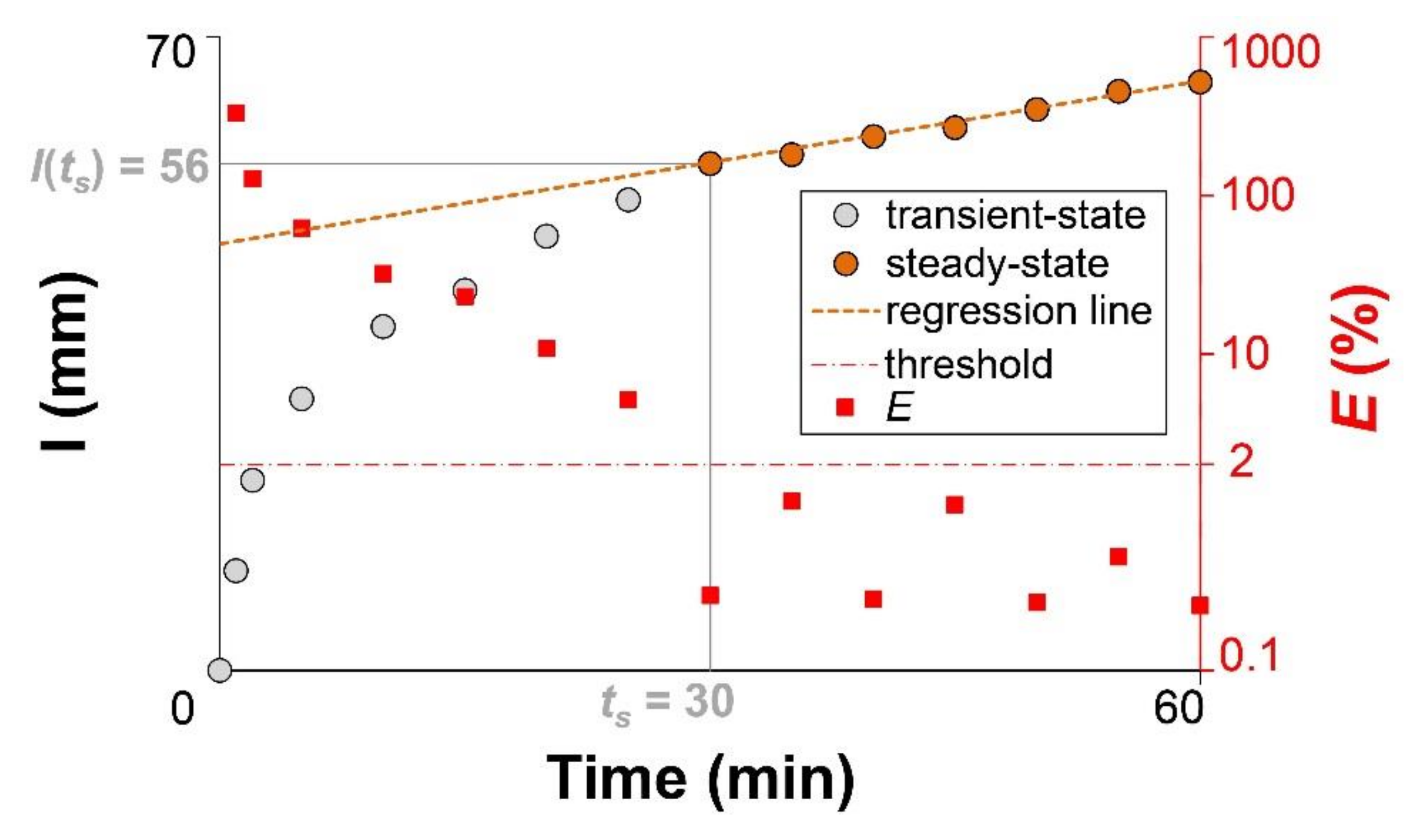
| ts (min) | 2012 | Control | 25 | 40 | 30.5 | 12.1 |
| Burnt | 25 | 45 | 35.0 | 22.3 | ||
| 2017 | Control | 20 | 50 | 33.5 | 29.9 | |
| Burnt | 15 | 45 | 32.5 | 32.6 | ||
| I(ts) (mm) | 2012 | Control | 29 | 86 | 61.9 | 22.0 |
| Burnt | 36 | 59 | 49.8 | 17.2 | ||
| 2017 | Control | 53 | 84 | 64.1 | 17.1 | |
| Burnt | 19 | 71 | 49.3 | 40.6 | ||
| Variable | Year | Site | Statistic | |||
|---|---|---|---|---|---|---|
| min | max | mean | CV | |||
| Ksf-BB | 2012 | Control | 1.52 | 4.99 | 3.04 AB | 45.4 |
| Burnt | 2.49 | 4.99 | 3.96 A | 19.5 | ||
| 2017 | Control | 2.18 | 5.35 | 3.62 A | 31.6 | |
| Burnt | 0.83 | 8.01 | 2.00 B | 68.7 | ||
| Ksf-WU2 | 2012 | Control | 1.34 | 5.28 | 2.95 AB | 59.5 |
| Burnt | 2.64 | 5.16 | 4.21 A | 20.6 | ||
| 2017 | Control | 2.00 | 5.82 | 3.57 AB | 39.1 | |
| Burnt | 0.88 | 8.91 | 2.03 B | 74.7 | ||
| Ksf-OPD | 2012 | Control | 1.24 | 4.98 | 2.85 AB | 56.2 |
| Burnt | 2.49 | 4.98 | 3.91 A | 19.9 | ||
| 2017 | Control | 1.99 | 5.34 | 3.44 A | 35.0 | |
| Burnt | 0.83 | 7.97 | 1.92 B | 71.8 | ||
© 2018 by the authors. Licensee MDPI, Basel, Switzerland. This article is an open access article distributed under the terms and conditions of the Creative Commons Attribution (CC BY) license (http://creativecommons.org/licenses/by/4.0/).
Share and Cite
Di Prima, S.; Lassabatere, L.; Rodrigo-Comino, J.; Marrosu, R.; Pulido, M.; Angulo-Jaramillo, R.; Úbeda, X.; Keesstra, S.; Cerdà, A.; Pirastru, M. Comparing Transient and Steady-State Analysis of Single-Ring Infiltrometer Data for an Abandoned Field Affected by Fire in Eastern Spain. Water 2018, 10, 514. https://doi.org/10.3390/w10040514
Di Prima S, Lassabatere L, Rodrigo-Comino J, Marrosu R, Pulido M, Angulo-Jaramillo R, Úbeda X, Keesstra S, Cerdà A, Pirastru M. Comparing Transient and Steady-State Analysis of Single-Ring Infiltrometer Data for an Abandoned Field Affected by Fire in Eastern Spain. Water. 2018; 10(4):514. https://doi.org/10.3390/w10040514
Chicago/Turabian StyleDi Prima, Simone, Laurent Lassabatere, Jesús Rodrigo-Comino, Roberto Marrosu, Manuel Pulido, Rafael Angulo-Jaramillo, Xavier Úbeda, Saskia Keesstra, Artemi Cerdà, and Mario Pirastru. 2018. "Comparing Transient and Steady-State Analysis of Single-Ring Infiltrometer Data for an Abandoned Field Affected by Fire in Eastern Spain" Water 10, no. 4: 514. https://doi.org/10.3390/w10040514