PATs Operating in Water Networks under Unsteady Flow Conditions: Control Valve Manoeuvre and Overspeed Effect


1
Hydraulic and Environmental Engineering Department, Universitat Politècnica de València, 46022 Valencia, Spain
2
Civil Engineering, Architecture and Georesources Departament, CERIS, Instituto Superior Técnico, Universidade de Lisboa, 1049-001 Lisboa, Portugal
*
Author to whom correspondence should be addressed.
Water 2018, 10(4), 529; https://doi.org/10.3390/w10040529
Submission received: 8 March 2018
/
Revised: 6 April 2018
/
Accepted: 9 April 2018
/
Published: 23 April 2018
(This article belongs to the Special Issue Advances in Water Distribution Networks)
Abstract
:The knowledge of transient conditions in water pressurized networks equipped with pump as turbines (PATs) is of the utmost importance and necessary for the design and correct implementation of these new renewable solutions. This research characterizes the water hammer phenomenon in the design of PAT systems, emphasizing the transient events that can occur during a normal operation. This is based on project concerns towards a stable and efficient operation associated with the normal dynamic behaviour of flow control valve closure or by the induced overspeed effect. Basic concepts of mathematical modelling, characterization of control valve behaviour, damping effects in the wave propagation and runaway conditions of PATs are currently related to an inadequate design. The precise evaluation of basic operating rules depends upon the system and component type, as well as the required safety level during each operation.
1. Introduction
The need to increase the efficiency in pressurized water networks has allowed the development of new water management strategies in the last decades [1,2]. These strategies have focused on two different directions according to the water pressurized network type (i.e., pumped or gravity systems). In pump solutions, the efficiency increase in the network is directly correlated with the reduction of the manometric head [3,4], the correction of operation rules and the design of facilities (e.g., pump efficiency, leakage control and the establishment of optimum schedules) [5]. In gravity systems, the efficiency improvement is related to the reduction of the leakage level through the installation of pressure reduction valves [6,7,8,9,10]. Ramos and Borga (1999) proposed the replacement of pressure reduction valves (PRVs) by hydraulic machines, which could also generate energy [11]. These systems provide two benefits: on the one hand, PATs reduce the pressure in the system and therefore, the leakages are also reduced by the operation of PRVs; on the other hand, the generated energy contributes to the improvement of the energy balance of these water systems, increasing the efficiency in the water networks, as well as improving performance indicators [12]. PATs can be used in any pipe system with excess of flow energy being more suitable for: (1) water supply networks, (2) irrigation systems, (3) industry processes, (4) drainage or storm systems and (5) treatment plants or at the entrance of reservoirs/tanks. The range operation (i.e., flow and head) is high and depends on the selected machine (i.e., radial, axial, mixed and multistage). Commonly, the flow rate is between 1 and 100 l/s and the head rate oscillates between 1 and 80 m w.c. (meters water column) However, it is possible to reach higher flows and heads if the machines are installed in parallel or in series. A deep analysis of the use of PATs in pipe systems, as well as the operation rate was described by [12]. Therefore, the success of PATs is related to the high operation rate and their combination (parallel or series), enabling the installation of these recovery machines where traditional turbines are not suitable.
Commonly, when replacing PRVs, a proposed hydraulic machine is a PAT [6]. Numerous researchers analysed the behaviour of these machines under steady flow conditions. A review of available technologies was conducted by different researchers [12,13,14,15]. A PAT analysis of performance and modelling was done on different hydraulic machines [14,16,17,18,19], while the computational analysis of these machines in a water distribution network was also studied [20,21,22,23]. The design of innovative strategies to maximize the recovered energy when the flows vary along a day, as well as their economic feasibility [24,25,26,27], in which the computed payback period achieved values between 2–12 years, depending on the system characteristics, was presented. Therefore, although the PAT installation is generally feasible, there are some cases in which the investment is economically unfeasible [28]. These strategies were applied to determine and maximize the theoretical recovered energy in both drinking and irrigation water systems [29,30]. The last case studies consider the significance of the flow change over time to predict the generated power in these facilities when they are installed in water systems [31]. The variability of the PATs performance as a function of flow, the maximization of the recovered energy that was developed using optimization procedures, and the economic analysis were successfully introduced in the analysis of a water pressurized system [32].
However, the study of the unsteady flow is poorly analysed in these systems and the installation of PATs encourages the need to know more about this subject. The transient analysis allows the estimation of the overpressures that could risk hydraulic facilities [33,34]. As a novelty, this research analyses the effective percentage of closure (effective %) in valve manoeuvres, the start-up and shutdown of radial and axial PATs with low inertia (i.e., of small sizes), as well as the runaway conditions induced by the overspeed effect through experimental data collection.
2. Material and Methods
2.1. Basic Hydraulic Modelling of the Transient Conditions
The unsteady flow can be analysed by a one-dimensional (1D) model type in pressurized pipe systems with higher length than diameter, using the mass and momentum conservation equations which are derived from the Reynolds transport theorem [35]. These principles are defined by differential Equations (1) and (2) [36,37,38,39]:
where H is the piezometric head in m; t is the time in s; c is the pressure wave speed in m/s, which is defined by the Equation (3); is the gravity acceleration in m/s2; A is the inner area of the pipe in m2; is the flow in m3/s; x is the coordinate along the pipeline axis; is the shear stress at the pipe wall in N/m2; is the density of the fluid in kg/m3; and is the inner diameter of the pipe in m.
where K is the fluid bulk modulus of elasticity in N/m2; E is the Young’s modulus of elasticity of the pipe in N/m2; and is the dimensionless parameter that takes into account the cross-section parameter of the pipe and supports constraint.
The considered assumptions applied in the classical, one dimensional, water hammer models are [37,38,39]:
- The flow is homogenous and compressible;
- The changes of density and temperature in the fluid are considered negligible when these are compared to pressure and flow variations;
- The velocity profile is considered pseudo-uniform in each section, assuming the values of momentum and Coriolis coefficients constant are equal to one;
- The behaviour of the pipe material is considered linear elastic;
- Head-losses are calculated by uniform flow friction formula, which is used in steady flow.
The differential Equations (1) and (2) can be simplified into a hyperbolic system of equations [36,39]. These equations can be presented as a matrix (4):
being:
where J is the hydraulic gradient.
The solution of these equations is obtained through a discretized time interval for each time step ‘Δt’ at a specific point of the pipe for each ‘x’, fulfilling the Courant condition (Cr = 1) (6):
The differential Equation (4) can be transformed into linear algebraic equations, obtaining Equations (7) and (8). The application of these equations is denominated the “Method of Characteristics” (MOC).
where is the piezometric head in m w.c. at pipe section “i” and time instant “n + 1”; is the velocity in m/s at pipe section “i” and time instant “n + 1”; where is the piezometric head in mw.c. at pipe section “i − 1” and time instant “n”; is the velocity in m/s at pipe section “i − 1” and time instant “n”; is the friction factor in the section “i − 1” at time instant “n”.
2.2. Control Valves
The valves are system components, which are responsible for changing the flow when its opening degree changes. Any operation in a valve modifies the opening degree and varies the loss coefficient of the valve causing a flow variation in the system, being one of the origin for hydraulic transients events. The closure time as well as the valve type influence the type of water hammer (i.e., fast or slow manoeuvers) for a system characterized by its diameter, length and pipe material.
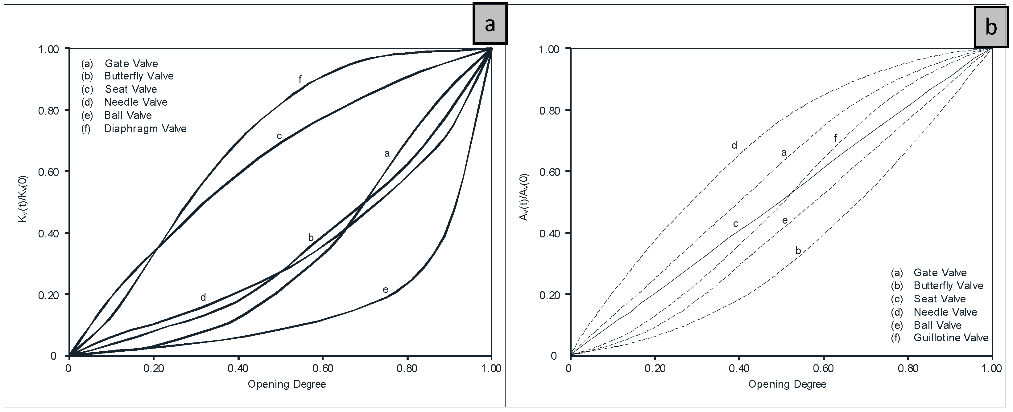
For any manoeuvre, the loss coefficient of the valve is function of the opening degree [40] and in a simplistic characterization, the behaviour of the valve can be defined by the Equation (9):
Figure 1 shows different closures as function of b exponent. If the exponent is one, the closure law is linear and the variation of the flow loss coefficient is continuous. When the exponent is less than one, the variation of the flow loss coefficient is higher at the end of the closure time (e.g., diaphragm valve-Figure 1a(f)). This significant difference in the loss coefficients (Kv) for different opening degrees will change the effective time closure defined in the Equation (10).
If the exponent is greater than one, the closure is higher at the beginning of the manoeuvre (e.g., butterfly valve), can cause higher overpressures since the main closure occurs when the velocity of the fluid is greater [41,42]. Although the closure law depends on the opening degree, by knowing the ratio of the free area as a function of the opening degree, the type of valve has great significance in the generated transient in a pipe system.
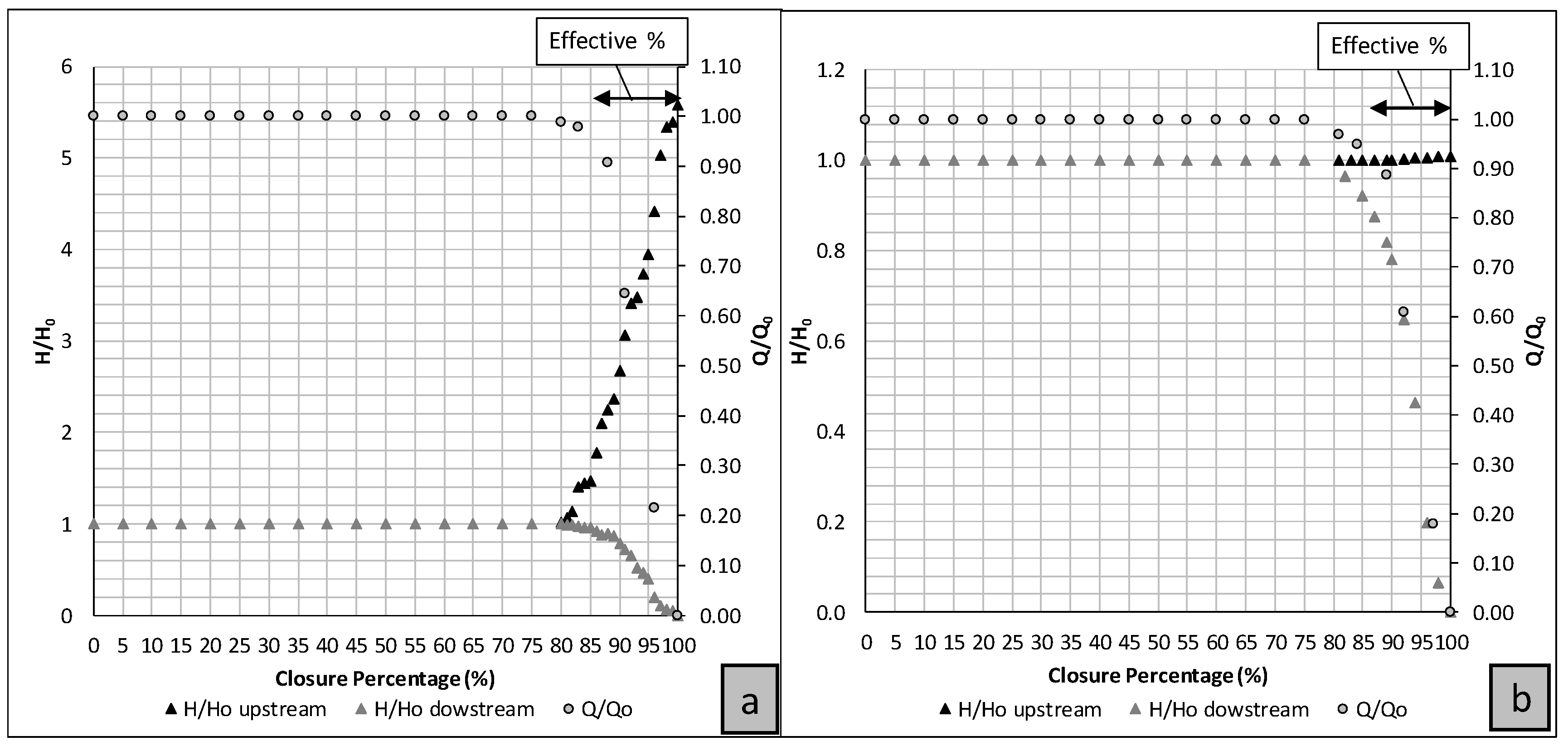
The duration of the valve manoeuvre, the diameter, the type of closure law (linear or non-linear) and the actuator type will influence the shape and values of the piezometric line envelopes. The effective time closure (Tef) is the real time of valve closure (shorter than the total time (TC)), which can induce high discharge reduction, responsible for the extreme water hammer phenomenon (as presented in Figure 2). Equation (10) mathematically defines the effective time closure based on the tangent to the point of the curvature in which dq/dt is highest:
where is the discharge variation in the hydraulic system, q is the ratio / (relative discharge value) and is the discharge for total opening.
2.3. Damping Effects
Water hammer analysis usually focuses on the estimation of the extreme pressures associated with the valve manoeuvre, the pump trip-off or the turbine shutdown or start-up. The correct prediction of the pressure wave propagation, in particular, the damping effect, is not always properly accounted for. The latter will influence the system re-operation, the model calibration and the dynamic behaviour of the system response. Currently, transient solvers commercially available are not able to predict the observed damping pressure surge in real systems.
A new simplified approach of surge damping is presented considering the pressure peak damping in time. This damping can be a combined effect of the non-elastic behaviour of the pipe-wall and the unsteady friction effect, depending essentially upon the pipe material [43]. This technique aims at the characterization of energy dissipation through the variation of the extreme piezometric head over time [6,43,44,45].
In a rigid pipe with an elastic behaviour, the energy dissipation of the system over time for a rough turbulent flow, in a dimensionless form, varies with h2 (due to almost exclusively friction effects). Based on the well-known upsurge given by the Joukowsky formulation through Equation (11):
where c is the celerity wave in m/s; is the flow in m3/s; g is gravity constant in m/s2 and S is the section of the pipeline (m2), the time head variation () can be obtained according to Equation (12):
assuming , being h0 the dimensionless head at initial time, , and the time for the first pressure peak where the head is maximum.
According to the same type of analysis, in a plastic pipe with a non-elastic behaviour (e.g., PVC, HDPE), the pipe-wall retarded-behaviour is mainly responsible for the pressure damping. Thus, the energy dissipation can adequately be reproduced with mathematic transformations using Equation (13) [43,44]:
This equation is in accordance with the typical behaviour of a viscoelastic solid. For systems with combined effects (i.e., elastic and plastic), the surge damping can be evaluated by the combination of both former effects through Equation (14) [43,44]
where Kplas and Kelas are decay coefficients for the plastic and elastic effects, respectively.
2.4. Runaway Conditions
The specific rotational speed (ns) given by Equation (15):
where is the specific speed of the machine in (m, kW); n is the rotational speed of the machine in rpm; P is the power in the shaft, which is measured in (kW); and H is the recovered head in (m w.c.), a characteristic parameter describing the runner shape and its associated dynamic behavior. The flow drops with the transient overspeed in reaction turbines with low specific speed. Conversely, the transient discharge tends to increase for turbines with high specific speed [6,35,44,45,46,47,48,49].
The flow across a runner is characterized by three types of velocities: absolute velocity of the water (V) with the direction imposed by the guide vane blade, relative velocity (W) through the runner and tangential velocity (C) of the runner.
If a uniform velocity distribution is assumed at inlet (Section 1) and outlet (Section 2) of a runner, the application of Euler’s theorem enables us to obtain the relation between the motor binary and the momentum moment between Section 1 and Section 2 by Equation (16):
where and r are the angle and radius, respectively (Figure 3).
The output power in the shaft is defined by Equation (17).
where BH is the hydraulic torque in Nm and P the output power in W.
3. Results and Discussion
3.1. Experiments and Simulations
The identification of turbomachines that can be used in pressurized systems are of action or reaction types. In the reaction machines, the hydraulic power is transmitted to the axis of the machine by varying the pressure flow between the inlet and outlet of the impeller, which depends on the specific speed of the machine (e.g., Francis, propeller and Kaplan). In action turbines, the energy exchange (hydraulic to mechanical) is carried out at atmospheric pressure, and the hydraulic power is due to the kinetic energy of the flow (e.g., Pelton and Turgo).
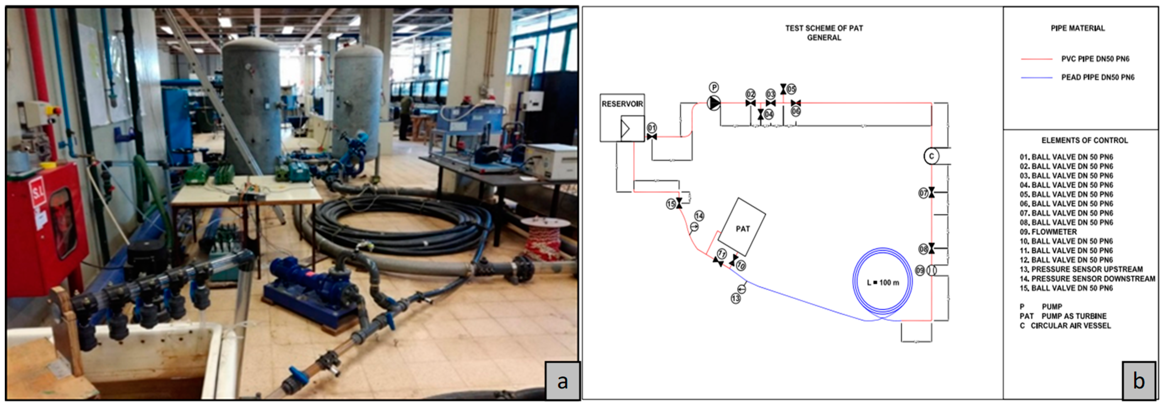
Experimental tests were carried out in the CERIS-Hydraulic Lab of Instituto Superior Técnico from the University of Lisbon for a radial and an axial reaction machine with small size (Figure 6a). A small pressurized system was installed in order to develop the experimental test. The facility scheme (Figure 6b) is composed of: (1) a reservoir to collect and supply the water looped facility; (2) one pump to recirculate the flow; (3) an air vessel to guarantee the uniform pressure in the pipe gravity system; (4) 100 m of HDPE pipeline or 25 m of PVC pipe for experiments with radial or axial PAT, respectively; (5) a radial or axial PAT depending on the selected machine. In both cases, the discharge was measured by an electromagnetic flowmeter; the pressure was registered by pressure transducers, through the Picoscope data acquisition system; the power was measured by a Wattmeter which was connected to the generator; and the rotational speed was measured by a frequency meter.
The used machines were a radial pump working as turbine (PAT), with a rotational specific speed of 51 rpm (in m, kW); and an axial one, with a rotational specific speed of 283 rpm (in m, kW) (Figure 7). Each machine was tested on different hydraulic circuits according to the available facilities. The radial machine scheme was composed of a reservoir to stabilize the flow; a pump to recirculate the flow; an air-vessel tank to control and stabilize the system pressure, which had a 1 m3 capacity; an electromagnetic flowmeter; one hundred meters of high density polyethylene (HDPE) pipe, with 50 mm nominal diameter; a PAT which is connected downstream of the HDPE loop pipe; and a ball valve located downstream of the PAT.
The ball valve was connected to the reservoir by a PVC pipe. The pump and air vessel were joined by a PVC pipe of 7.40 m of length and 50 mm of nominal diameter. The air vessel and flowmeter were joined by another rigid PVC pipe 1.80 m long. Two pressure sensors were installed upstream and downstream of the PAT to estimate the net head.
For the axial machine, the scheme was similar to the previous one. The facility was composed of a reservoir, a pump to recirculate the flow, an air vessel tank to maintain a quasi-uniform pressure (the capacity of this tank is 1 m3), an electromagnetic flowmeter to measure the flow and the axial machine, which is followed by a butterfly valve to isolate the facility. The pump and the air vessel were joined by a steel pipe with a length of 3.50 m and diameter of 80 mm. The axial machine and the butterfly valve were connected by a pipe, which is composed of PVC (4.90 m and 110 mm of diameter) and a steel pipe (4.50 m and 80 mm of diameter). The butterfly valve and the reservoir were connected by a steel pipe, 2 m long, with a diameter equal to 80 mm. Two pressure sensors were installed upstream and downstream of the axial machine.
These hydraulic systems (Figure 8) were simulated by Allievi software [51] according to the system characteristics in each facility, previously described. The inner diameter and the wave speed are shown in Table 1 according to the pipe material. During the simulation process, all singularities were verified and the friction losses along the pipe system were defined, adopting the following procedure with excellent results: (1) a model calibration for the friction factor (pipe roughness) and for the singular head losses was done, considering different singularities, such as ball valves, inlet and outlet of the air-vessel, elbows, bifurcations and valve connections; this setting under steady state conditions that allowed us to make small refinements after comparisons with the experiments; (2) due to the system characteristics, it was also possible to fit the damping effect, as well as the phase shift of the pressure waves during unsteady state conditions; based on the authors experience, it was concluded that in viscoelastic pipes and for slow manoeuvres, the unsteady friction has no significance in terms of the damping and the shape of the pressure wave propagation. The dynamic mathematical model considers the internal friction losses to analyse the presence of a PAT in a water distribution network with suitable results [46,47].
The simulated flow and the head in the pump, as well as the pressure in the air vessel, were calibrated in each developed simulation (i.e., for radial and axial machines) according to the registered experimental data for each test type. When the radial machine was tested, the flow values oscillated between 1 and 7 l/s, the upstream pressure between 15 and 30 m, and the head drop between 3 and 10 m. In the axial machine, the tested flow varied between 5 and 14.1 l/s, the upstream pressure between 10 and 20 m and the head drop between 0.25 and 7 m, as previously designed [20,50].
3.2. Control Valve Closure and PAT Trip-Off
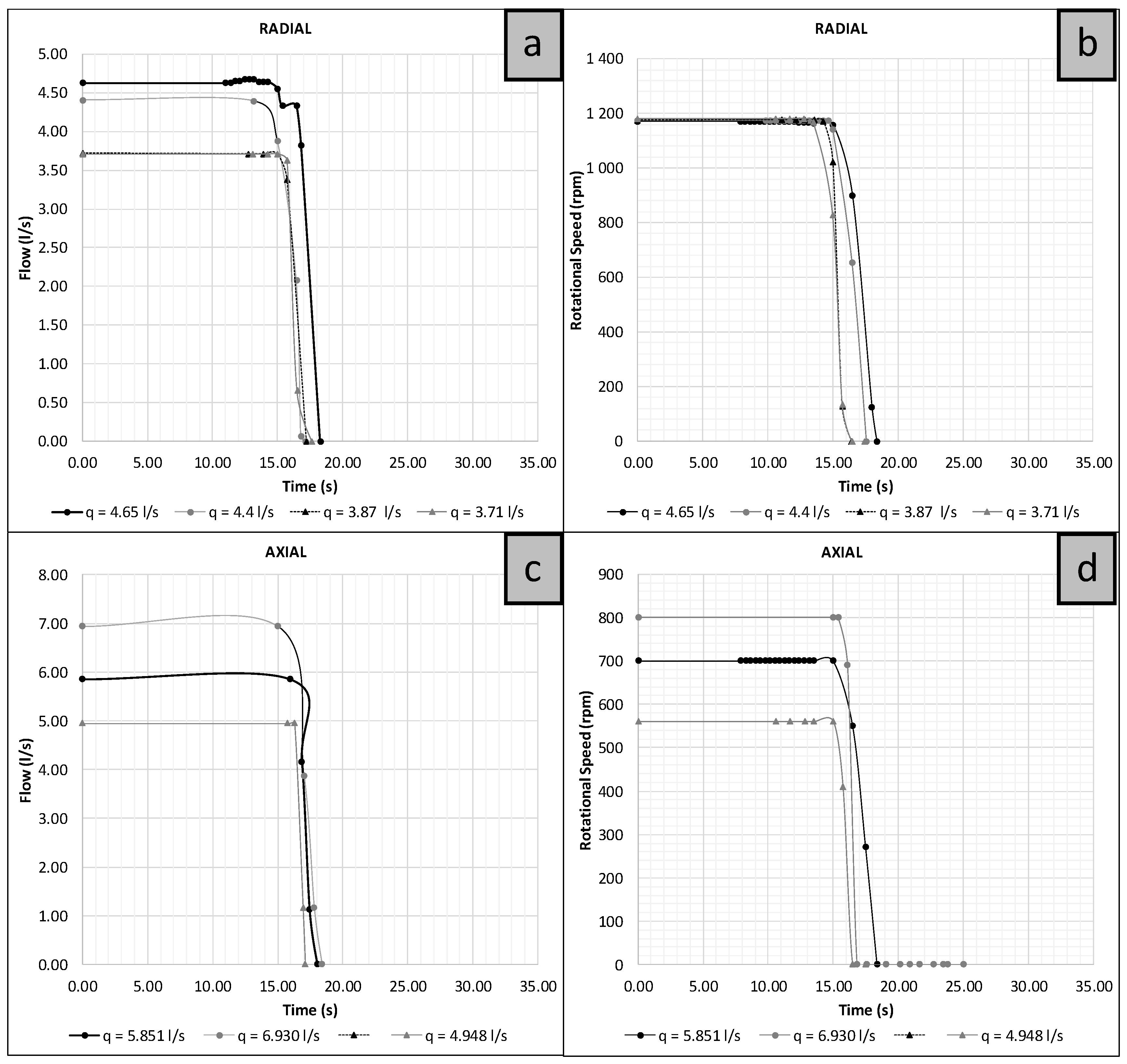
This section shows the flow and the rotational speed variation when a fast shutdown was carried out downstream of the PAT. Figure 9 shows four tests with different initial flow values in the radial machine and three tests for the axial one. The values rapidly varied from the nominal values (flow and rotational speed) to zero. The closure time is around two seconds in all considered manoeuvres.
According to the installed systems, the model was implemented in Allievi software as the scheme presented in Figure 8 shows. The software is a computational model that enables us to analyse water systems (pressurized and open channel flows) under steady and unsteady conditions. The developed model was calibrated to consider the damping effects that were associated with the characteristic parameters of the system, as well as the type of hydraulic machines.
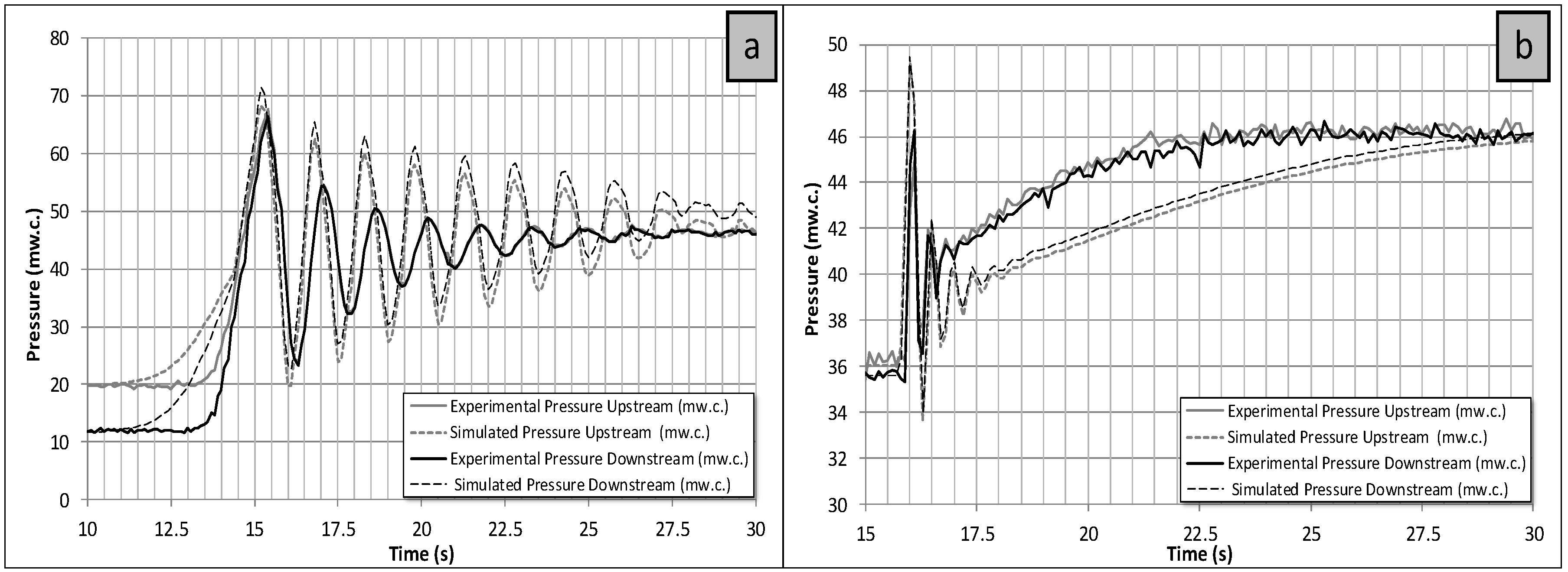
Comparisons between experimental and simulated pressure values (upstream and downstream) presented adequate fitting. In Figure 10, the experimental overpressure in the radial machine was 69.85 m w.c. while the simulated overpressure was 70.52 m w.c. The result in the first depression wave was similar, where the minimum experimental value was 24.54 m w.c. and the simulated was 19.73 m w.c. The axial machine presented values of 46.23 m w.c. (experimental) and 49.24 m w.c. (simulated). The minimum experimental depression value was 36.54 m w.c. while the simulated value was 33.63 m w.c. These results showed the dynamic behaviour of the radial and axial machines when a downstream induced transient attained the turbine runner. The transient wave passed through the runners and the pressure variation upstream and downstream was essentially in phase.
3.3. Control Valve Opening and PAT Start-Up
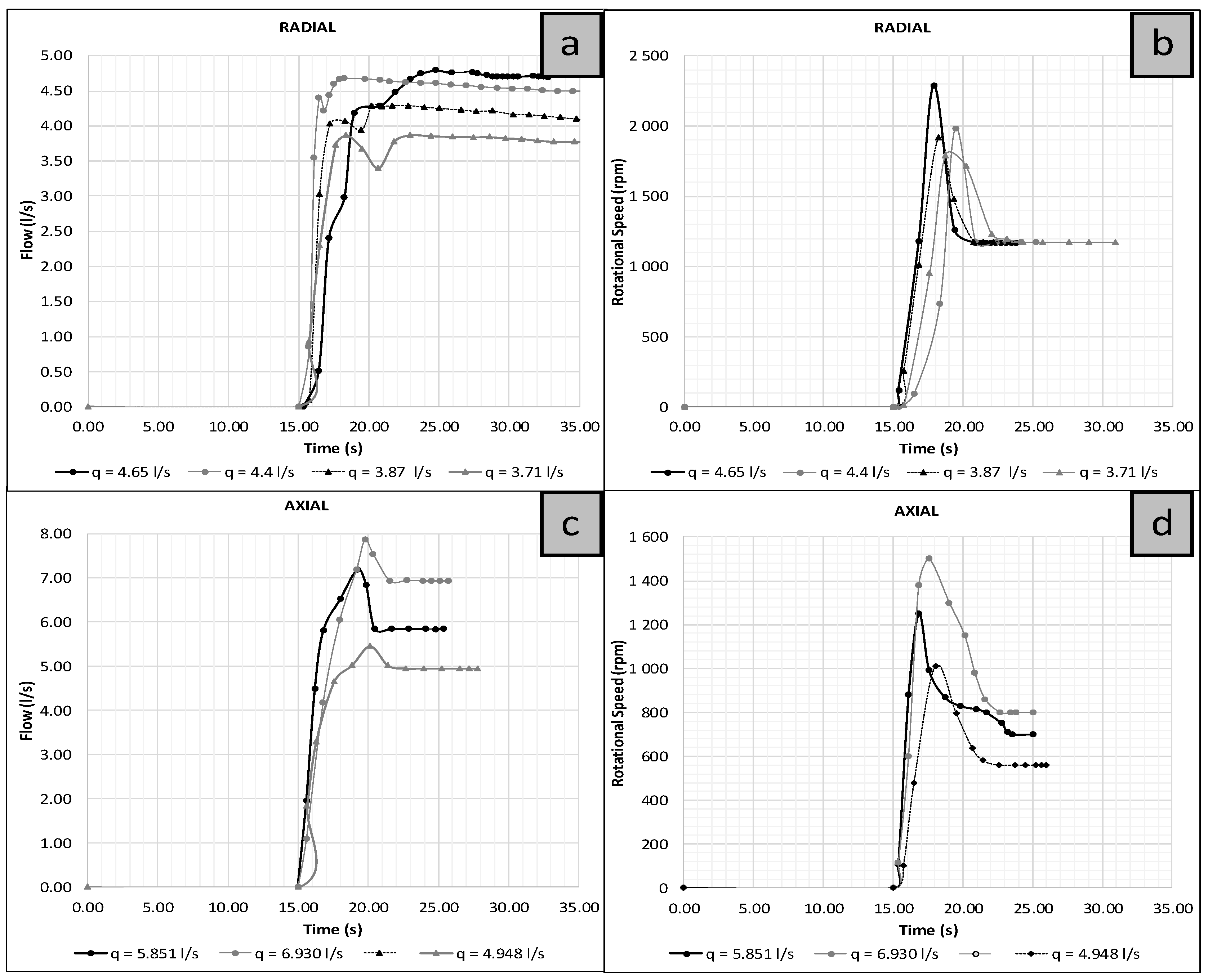
The flow, the rotational speed, and the pressure values (upstream and downstream) were recorded over time (Figure 11 and Figure 12). Figure 11 shows the flow and speed variation for a fast opening of the downstream control valve for each system. Some variations can be observed, where the rotational speed of the machine reached 2235 rpm. This value was double the nominal rotational speed of the machine for 4.65 l/s in the radial machine. The reached value was 1500 rpm for the axial machine, when the nominal flow and the nominal rotational speed were 6.93 l/s.
The trend in the valve opening for PAT start-up was similar in all cases: firstly, the machine increased the rotational speed upper its nominal value. When the overspeed was reached for flow value near 4.00 l/s (in radial machine) and 7.86 l/s (in axial machine), the rotational speed decreased to the nominal one. In this time, the flow attained the nominal flow with the maximum valve opening degree. A downsurge wave in both machines (radial and axial) was observed with the valve opening. This depression depended on the flow and the opening time. This value was also simulated with Allievi, achieving quite accurate results (Figure 12). The root mean square error (RMSE) for each simulation with Allievi was determined. The average RMSE obtained in the first phase of the water hammer phenomenon (i.e., worst value) was 2.37%, and the standard deviation was 3.47%. When the maximum downsurge and upsurge were compared to the experiments, the maximum error was 1.26%.
3.4. Overspeed Effect in PATs
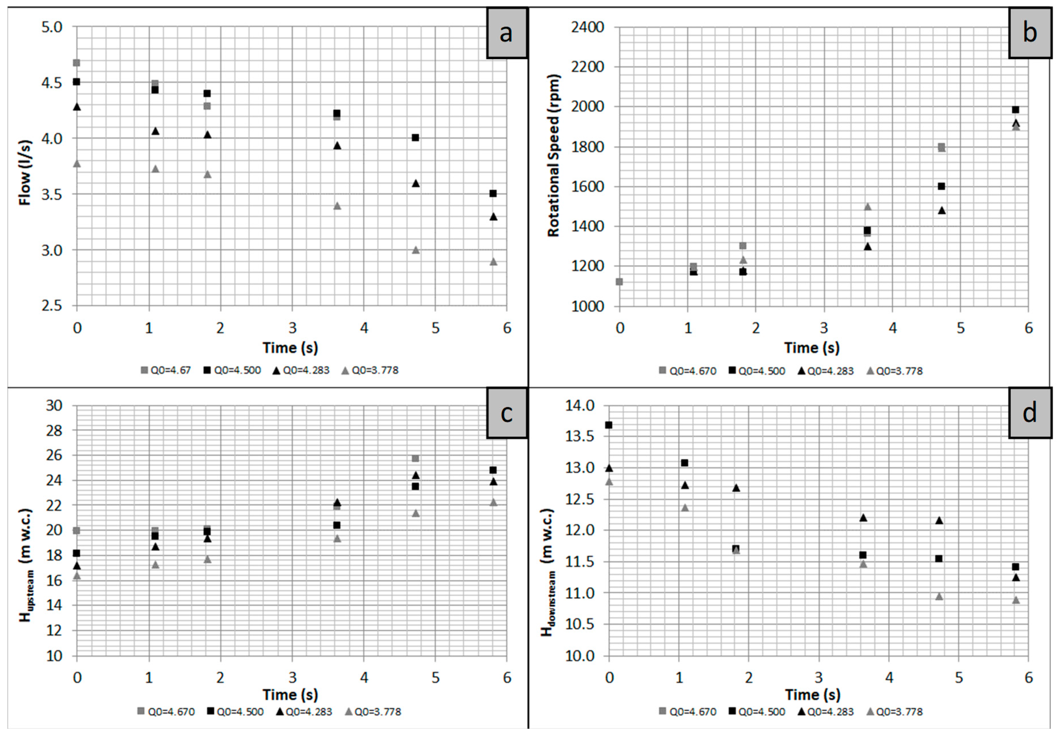
Some interesting conclusions can be drawn for both types of runners. Figure 13 presents the obtained values of flow, rotational speed, and pressure (upstream and downstream) for the overspeed conditions. The flow value decreased over time in all tests induced by the runner shape associated with the low specific speed value as previously mentioned from Figure 3, Figure 4 and Figure 5. This decrease of the flow was related to an increase in the rotational speed, with the minimum flow attained when the runaway conditions were reached.
Regarding the pressure variation, some issues can be observed: the upstream pressure value increased, resulting in the maximum pressure when the machine reaches the runaway conditions and consequently, the downstream pressure decreased (Figure 13). Therefore, the radial runner induced a flow cut effect under overspeed conditions.
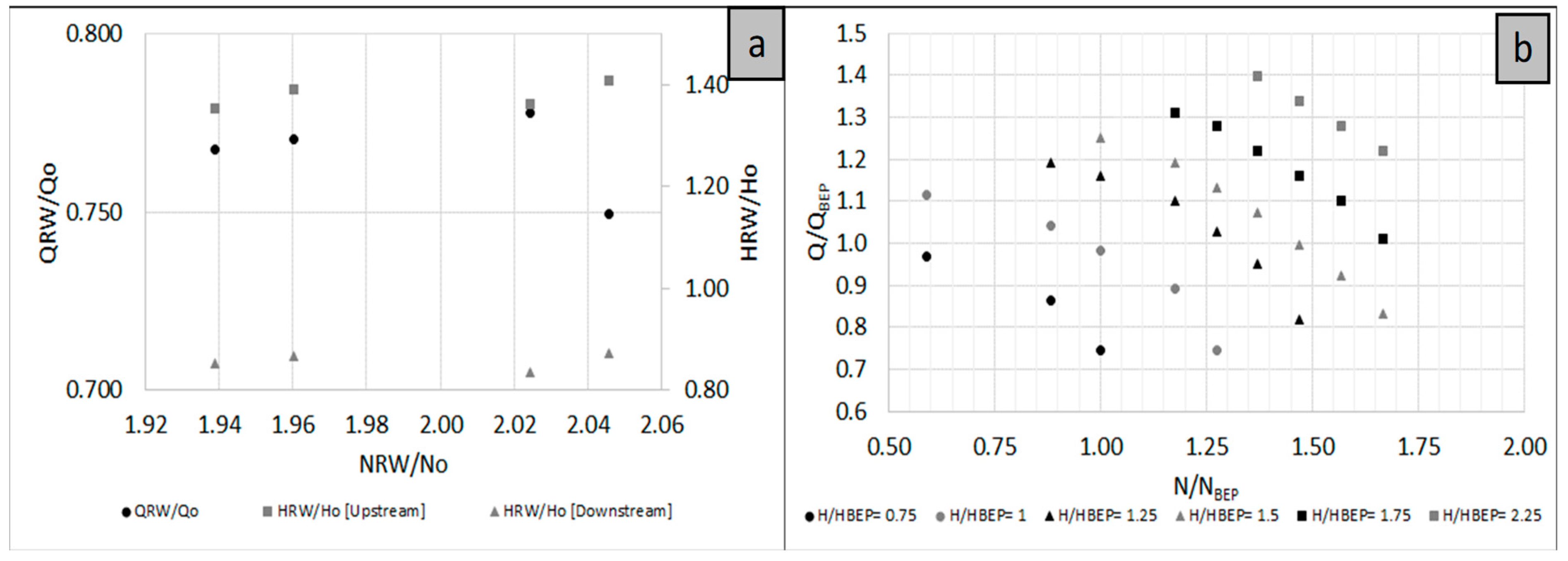
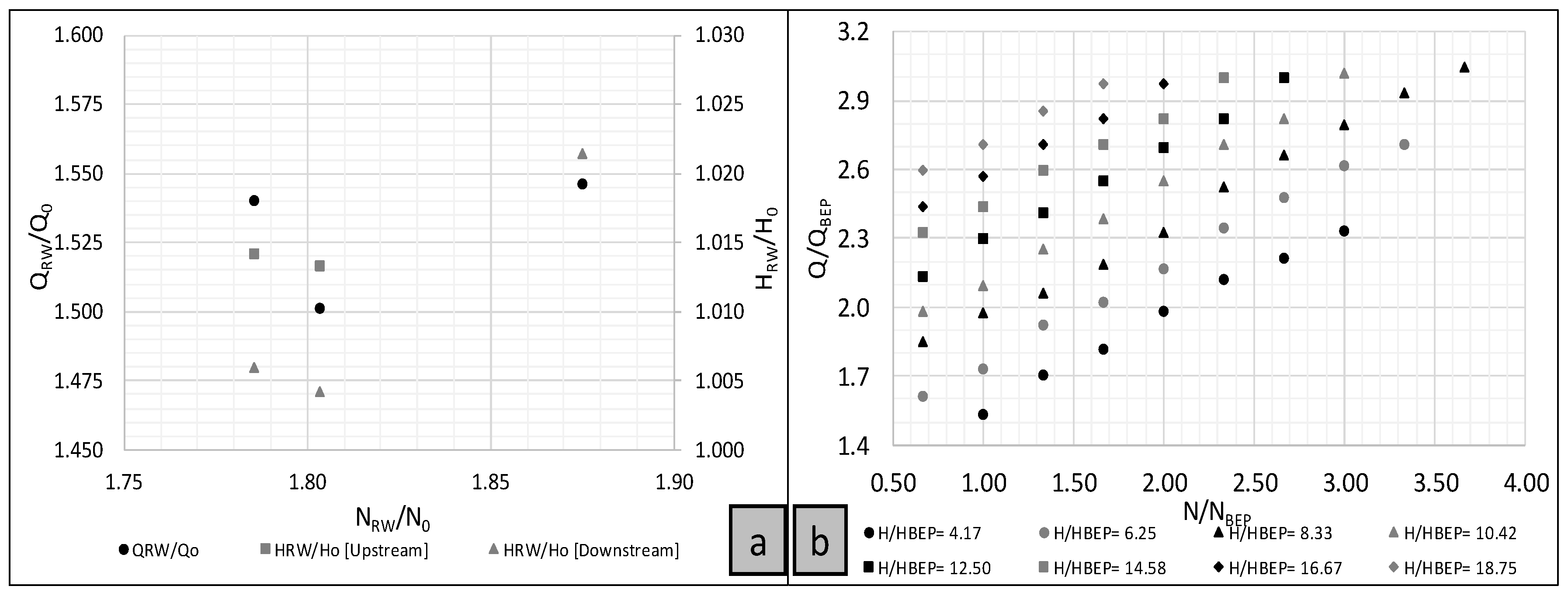
The experimental data under runaway conditions can be expressed by different parameters: the discharge flow, the pressure and the rotational speed for total opening valve degree (0, H0, N0). Furthermore, the experimental results can be associated with the values of the best efficiency point of the machine in turbine mode (BEP, HBEP, NBEP). These variations are shown in Figure 14. If RW/0 versus NRW/N0 (the subscripts ‘RW’ indicates runaway conditions) is observed, the values were almost constant for all experimental data denoting a typical characteristic of the radial machine. In this case, the ratio RW/0 is near 0.514; therefore, there was a flow reduction of around 50%. This value is close to the presented value in Figure 4 that shows the characteristic of the radial machine under the overspeed effect. Similar conclusions can be obtained if the upstream and downstream pressures are analysed in the axial machine. In this case, the values were near 1.40 and 0.85, inducing an upsurge and a downsurge upstream and downstream, respectively, of the machine. If the values are compared with the best efficiency point of the radial machine, under the overspeed effect, the flow decreased for a constant value of h (h = H/HBEP).
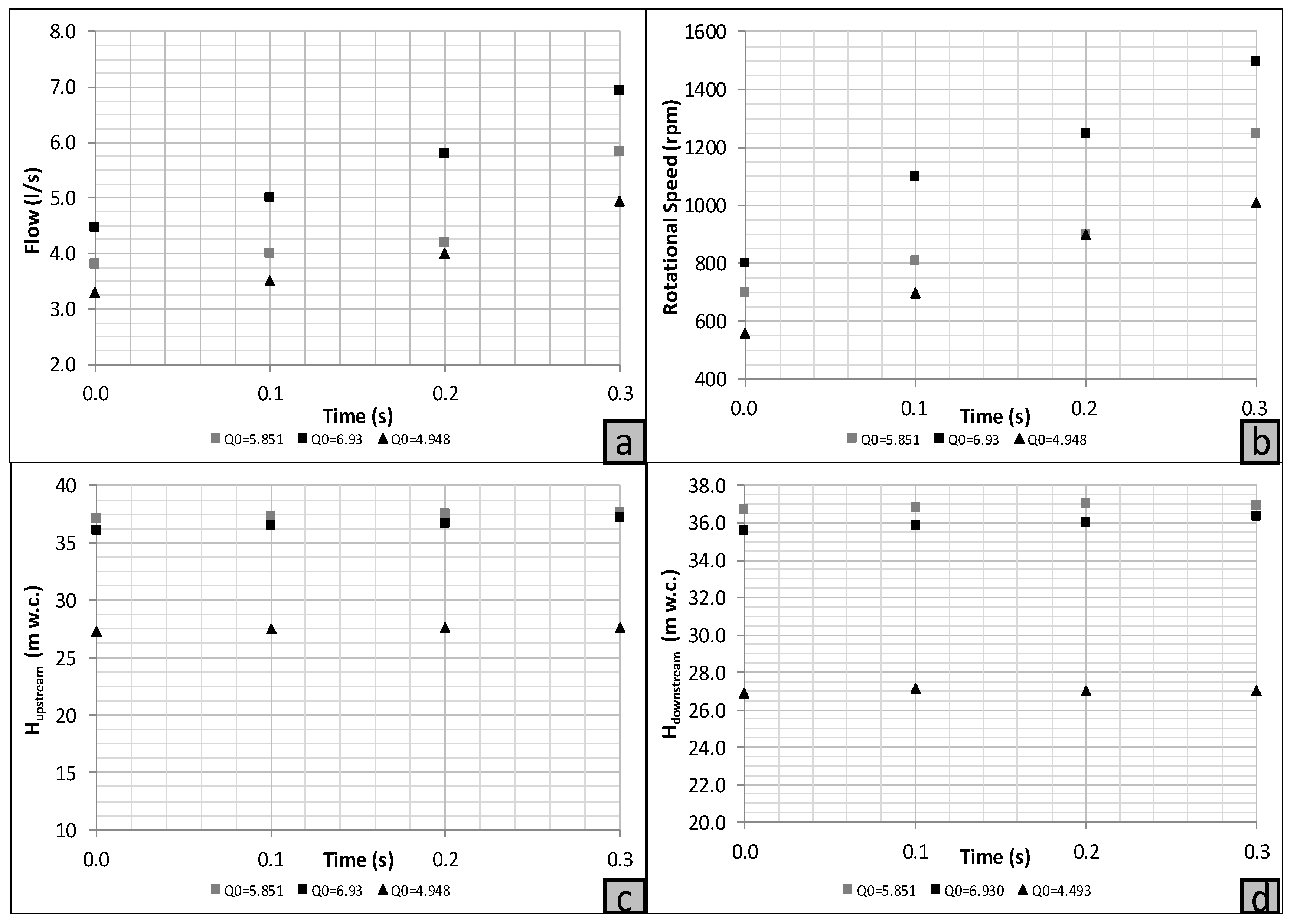
Converse results were obtained when the experimental data were analyzed for the axial machine (Figure 15). The flow rise over time as the rotational speed increased until to reach the runaway value. In these cases, the upstream and downstream pressures remained almost constant over time.
As for the radial machine, Figure 16 shows the experimental data for the discharge flow, pressure, and the rotational speed variation for the total valve opening (0, H0, N0) during the overspeed conditions of the axial machine. In this case, the ratio RW/0 showed an increase in flow. This value is higher than the obtained value using Figure 4, for ns of 280 rpm (in m, kW).
The experimental data were also correlated with the values of the best efficiency point (BEP, HBEP, NBEP). The results contrasted with those obtained for the radial machine. Under a constant value of h (h = H/HBEP), the flow increased when the rotational speed increased. Figure 16 shows all analysed cases considering a constant h value and they present the same tendency.
4. Conclusions
Based on the authors’ experience and laboratory tests, a large number of criteria to deal with the design and hydraulic transients of micro hydropower systems are addressed. The type of analysis will be influenced by the design stage and the complexity of each system. Hence, based on each hydraulic system characteristic, for the most predictable manoeuvres, the designers will be able to define exploitation rules according to expected safety levels. In fact, convenient operational rules need to be specified in order to control the maximum and minimum transient pressures. These specifications will mainly depend on the following factors:
- the characteristics of the pipe system to be protected; in fact, these characteristics based on the head loss and inertia of the water column can adversely modify the system behaviour and the same valve closure time can induce a slow or a rapid flow change;
- the intrinsic characteristics of the valve: a butterfly valve (e.g., for medium heads) and a spherical valve (e.g., for high heads) have different effects on the dynamic flow response for the same closure law;
- since PATs have no guide vane, the flow control is made through valves where the closure and opening laws are crucial in the safety system conditions, such as the type of the valve actuator;
- based on the characteristics of the pump such as turbine machine (i.e., radial or axial), different dynamic behaviour will be associated with:
- ○
- the small inertia of the rotating masses induces a fast overspeed effect under runaway conditions imposed by a full load rejection.
- ○
- the overspeed effects provoke flow variations (i.e., flow reduction in low ns machines and flow increasing in the high ns machines) and pressure variations that can propagate upsurges upstream of a radial machine and downsurges downstream of it, in contrast to axial machines (downsurges upstream and upsurges downstream).
As a novelty, the manuscript analyses the unsteady flow behaviour in real PATs system. This analysis is based on data obtained during an intensive experimental campaign, and important information is presented and utilized for some specific PAT transient state conditions, using a computational tool that was previously calibrated.
This analysis required a mathematical transformation of available data of pumps (based on experiments especially developed for this study) into characteristic curves of discharge variation, /BEP, with the rotating speed, N/NBEP (Figure 14 and Figure 16, for radial and axial machines, respectively). This procedure facilitates understanding of the dynamic pump as turbine behaviour under unsteady conditions.
The feasibility of pumps operating as turbines was proved, based on typical performed control analyses. The dynamic behaviour of those machines presents similarities to the classical reaction turbines, regarding the flow variation due to the runner type, generally characterized by its specific rotational speed (ns) [35,45,47,51] apart from the associated scale effects.
These PAT solutions can be adopted instead of energy dissipation devices in conveyance pipe systems with excess available energy at some pipe sections. Therefore, the use of reverse pumps in drinking, irrigation and sewage or drainage water systems can be a rather interesting solution in some cases, taking the advantage of the available head that in another way would be dissipated.
Author Contributions
The author Helena M. Ramos has contributed with the idea, wrote part of the document, was in the revision of the document and supervised the whole research. Modesto Pérez-Sánchez did the experiments and wrote part of the document. P. Amparo López-Jiménez suggested guides towards the developed analyses.
Funding
The authors wish to thank to the project REDAWN (Reducing Energy Dependency in Atlantic Area Water Networks) EAPA_198/2016 from INTERREG ATLANTIC AREA PROGRAMME 2014–2020 and CERIS (CEHIDRO-IST). This research was developed in the research stay of the first author in the hydraulic lab of CERIS-IST in January 2018 called “MAXIMIZATION OF THE GLOBAL EFFICIENCY IN PATs IN LABORATORY FACILITY”.
Conflicts of Interest
The authors have declared that no competing interests exist.
References
- Kougias, I.; Patsialis, T.; Zafirakou, A.; Theodossiou, N. Exploring the potential of energy recovery using micro hydropower systems in water supply systems. Water Util. J. 2014, 7, 25–33. [Google Scholar]
- Nogueira, M.; Perrella, J. Energy and hydraulic efficiency in conventional water supply systems. Renew. Sustain. Energy Rev. 2014, 30, 701–714. [Google Scholar] [CrossRef]
- Moreno, M.; Córcoles, J.; Tarjuelo, J.; Ortega, J. Energy efficiency of pressurised irrigation networks managed on-demand and under a rotation schedule. Biosyst. Eng. 2010, 107, 349–363. [Google Scholar] [CrossRef]
- Jiménez-Bello, M.A.; Royuela, A.; Manzano, J.; Prats, A.G.; Martínez-Alzamora, F. Methodology to improve water and energy use by proper irrigation scheduling in pressurised networks. Agric. Water Manag. 2015, 149, 91–101. [Google Scholar] [CrossRef]
- Cabrera, E.; Cabrera, E., Jr.; Cobacho, R.; Soriano, J. Towards an Energy Labelling of Pressurized Water Networks. Procedia Eng. 2014, 70, 209–217. [Google Scholar] [CrossRef]
- Carravetta, A.; Houreh, S.D.; Ramos, H.M. Pumps as Turbines: Fundamentals and Applications; Springer International Publishing: Cham, Switzerland, 2018; p. 218. ISBN 978-3-319-67507-7. [Google Scholar]
- Abbott, M.; Cohen, B. Productivity and efficiency in the water industry. Util. Policy 2009, 17, 233–244. [Google Scholar] [CrossRef]
- Araujo, L.; Ramos, H.; Coelho, S. Pressure Control for Leakage Minimisation in Water Distribution Systems Management. Water Resour. Manag. 2006, 20, 133–149. [Google Scholar] [CrossRef]
- Dannier, A.; Del Pizzo, A.; Giugni, M.; Fontana, N.; Marini, G.; Proto, D. Efficiency evaluation of a micro-generation system for energy recovery in water distribution networks. In Proceedings of the 2015 International Conference on Clean Electrical Power (ICCEP), Taormina, Italy, 16–18 June 2015; pp. 689–694. [Google Scholar]
- Giugni, M.; Fontana, N.; Ranucci, A. Optimal Location of PRVs and Turbines in Water Distribution Systems. J. Water Resour. Plan. Manag. 2014, 140, 06014004. [Google Scholar] [CrossRef]
- Ramos, H.; Borga, A. Pumps as turbines: An unconventional solution to energy production. Urban Water 1999, 1, 261–263. [Google Scholar] [CrossRef]
- Pérez-Sánchez, M.; Sánchez-Romero, F.; Ramos, H.; López-Jiménez, P.A. Energy Recovery in Existing Water Networks: Towards Greater Sustainability. Water 2017, 9, 97. [Google Scholar] [CrossRef]
- Senior, J.; Saenger, N.; Müller, G. New hydropower converters for very low-head differences. J. Hydraul. Res. 2010, 48, 703–714. [Google Scholar] [CrossRef]
- Razan, J.I.; Islam, R.S.; Hasan, R.; Hasan, S.; Islam, F. A Comprehensive Study of Micro-Hydropower Plant and Its Potential in Bangladesh. ISRN Renew. Energy 2012, 2012, 635396. [Google Scholar] [CrossRef]
- Elbatran, A.H.; Yaakob, O.B.; Ahmed, Y.M.; Shabara, H.M. Operation, performance and economic analysis of low head micro-hydropower turbines for rural and remote areas: A review. Renew. Sustain. Energy Rev. 2015, 43, 40–50. [Google Scholar] [CrossRef]
- Nourbakhsh, A.; Jahangiri, G. Inexpensive small hydropower stations for small areas of developing countries. In Proceedings of the Conference on Advanced in Planning-Design and Management of Irrigation Systems as Related to Sustainable Land Use, Louvain, Belgium, 14–17 September 1992; pp. 313–319. [Google Scholar]
- Simão, M.; Ramos, H.M. Hydrodynamic and performance of low power turbines: Conception, modelling and experimental tests. Int. J. Energy Environ. 2010, 1, 431–444. [Google Scholar]
- Arriaga, M. Pump as turbine—A pico-hydro alternative in Lao People’s Democratic Republic. Renew. Energy 2010, 35, 1109–1115. [Google Scholar] [CrossRef]
- Pérez-Sánchez, M.; López Jiménez, P.A.; Ramos, H.M. Modified Affinity Laws in Hydraulic Machines towards the Best Efficiency Line. Water Resour. Manag. 2018, 3, 829–844. [Google Scholar] [CrossRef]
- Ramos, H.M.; Borga, A.; Simão, M. New design solutions for low-power energy production in water pipe systems. Water Sci. Eng. 2009, 2, 69–84. [Google Scholar]
- Carravetta, A.; Del Giudice, G.; Fecarotta, O.; Ramos, H.M. Energy Recovery in Water Systems by PATs: A Comparisons among the Different Installation Schemes. Procedia Eng. 2014, 70, 275–284. [Google Scholar] [CrossRef]
- Caxaria, G.; de Mesquita e Sousa, D.; Ramos, H.M. Small Scale Hydropower: Generator Analysis and Optimization for Water Supply Systems. 2011, p. 1386. Available online: http://www.ep.liu.se/ecp_article/index.en.aspx?issue=57;vol=6;article=2 (accessed on 12 March 2017).
- Butera, I.; Balestra, R. Estimation of the hydropower potential of irrigation networks. Renew. Sustain. Energy Rev. 2015, 48, 140–151. [Google Scholar] [CrossRef]
- Carravetta, A.; Fecarotta, O.; Del Giudice, G.; Ramos, H. PAT Design Strategy for Energy Recovery in Water Distribution Networks by Electrical Regulation. Energies 2013, 6, 411–424. [Google Scholar] [CrossRef]
- Fecarotta, O.; Aricò, C.; Carravetta, A.; Martino, R.; Ramos, H.M. Hydropower Potential in Water Distribution Networks: Pressure Control by PATs. Water Resour. Manag. 2014, 29, 699–714. [Google Scholar] [CrossRef] [Green Version]
- Fecarotta, O.; Carravetta, A.; Ramos, H.M.; Martino, R. An improved affinity model to enhance variable operating strategy for pumps used as turbines. J. Hydraul. Res. 2016, 54, 332–341. [Google Scholar] [CrossRef]
- Sitzenfrei, R.; Berger, D.; Rauch, W. Design and optimization of small hydropower systems in water distribution networks under consideration of rehabilitation measures. Urban Water J. 2015, 12, 1–9. [Google Scholar] [CrossRef]
- De Marchis, M.; Milici, B.; Volpe, R.; Messineo, A. Energy Saving in Water Distribution Network through Pump as Turbine Generators: Economic and Environmental Analysis. Energies 2016, 9, 877. [Google Scholar] [CrossRef]
- Samora, I.; Manso, P.; Franca, M.; Schleiss, A.; Ramos, H. Energy Recovery Using Micro-Hydropower Technology in Water Supply Systems: The Case Study of the City of Fribourg. Water 2016, 8, 344. [Google Scholar] [CrossRef]
- Pérez-Sánchez, M.; Sánchez-Romero, F.; Ramos, H.; López-Jiménez, P.A. Modeling Irrigation Networks for the Quantification of Potential Energy Recovering: A Case Study. Water 2016, 8, 234. [Google Scholar] [CrossRef]
- Corcoran, L.; McNabola, A.; Coughlan, P. Predicting and quantifying the effect of variations in long-term water demand on micro-hydropower energy recovery in water supply networks. Urban Water J. 2016, 9, 1–9. [Google Scholar] [CrossRef]
- Pérez-Sánchez, M.; Sánchez-Romero, F.J.; Ramos, H.M.; López Jiménez, P.A. Optimization Strategy for Improving the Energy Efficiency of Irrigation Systems by Micro Hydropower: Practical Application. Water 2017, 9, 799. [Google Scholar] [CrossRef]
- Imbernón, J.A.; Usquin, B. Sistemas de generación hidráulica. Una nueva forma de entender la energía. In Proceedings of the II Congreso Smart Grid, Madrid, Spain, 27–28 October 2014. [Google Scholar]
- McNabola, A.; Coughlan, P.; Corcoran, L.; Power, C.; Prysor, A.; Harris, I.; Gallagher, J.; Styles, D. Energy recovery in the water industry using micro-hydropower: An opportunity to improve sustainability. Water Policy 2014, 16, 168–183. [Google Scholar] [CrossRef]
- Ramos, H. Simulation and Control of Hydrotransients at Small Hydroelectric Power Plants. Ph.D. Thesis, IST, Lisbon, Portugal, December 1995. [Google Scholar]
- White, F.M. Fluid Mechanics, 6th ed.; McGrau-Hill: New York, NY, USA, 2008. [Google Scholar]
- Wylie, E.B.; Streeter, V.L. Fluid Transients in Systems; Prentice Hall: Englewood Cliffs, NI, USA, 1993. [Google Scholar]
- Almeida, A.B.; Koelle, E. Fluid Transients in Pipe Networks; Computational Mechanics Publications, Elsevier Applied Science: Amsterdam, The Netherlands, 1992. [Google Scholar]
- Chaudhry, M. Applied Hydraulic Transients, 2nd ed.; Springer-Verlag: New York, NY, USA, 1987. [Google Scholar]
- Abreu, J.; Guarga, R.; Izquierdo, J. Transitorios y Oscilaciones en Sistemas Hidráulicos a Presión; Abreu, J., Guarga, R., Izquierdo, J., Eds.; U.D. Mecánica de Fluidos, Universidad Politécnica de Valencia: Valencia, Spain, 1995. [Google Scholar]
- Iglesias-Rey, P.; Izquierdo, J.; Fuertes, V.; Martínez-Solano, F. Modelación de Transitorios Hidráulicos Mediante Ordenador; Grupo Mult.; Universidad Politécnica de Valencia: Valencia, Spain, 2004. [Google Scholar]
- Subani, N.; Amin, N. Analysis of Water Hammer with Different Closing Valve Laws on Transient Flow of Hydrogen-Natural Gas Mixture. Abstr. Appl. Anal. 2015, 2, 12–19. [Google Scholar] [CrossRef]
- Ramos, H.M.; Covas, D.; Borga, A.; Loureiro, D. Surge damping analysis in pipe systems: Modelling and experiments. J. Hydraul. Res. 2004, 42, 413–425. [Google Scholar] [CrossRef]
- Ramos, H. Design concerns in pipe systems for safe operation. Dam Eng. 2003, 14, 5–30. [Google Scholar]
- Ramos, H. Guidelines for Design of Small Hydropower Plants; Western Regional Energy Agency & Network (WREAN); Department of Economic Development (DED): Belfast, UK, 2000. [Google Scholar]
- Ramos, H.; Almeida, A.B. Dynamic orifice model on water hammer analysis of high or medium heads of small hydropower schemes. J. Hydraul. Res. 2001, 39, 429–436. [Google Scholar] [CrossRef]
- Ramos, H.; Almeida, A.B. Parametric Analysis of Water-Hammer Effects in Small Hydro Schemes. J. Hydraul. Eng. 2002, 128, 689–696. [Google Scholar] [CrossRef]
- Ramos, H.M.; Simão, M.; Borga, A. Experiments and CFD Analyses for a New Reaction Microhydro Propeller with Five Blades. J. Energy Eng. 2013, 139, 109–117. [Google Scholar] [CrossRef]
- Mataix, C. Turbomáquinas Hidráulicas; Universidad Pontificia Comillas: Madrid, Spain, 2009. [Google Scholar]
- De Marchis, M.; Fontanazza, C.M.; Freni, G.; Messineo, A.; Milici, B.; Napoli, E.; Notaro, V.; Puleo, V.; Scopa, A. Energy recovery in water distribution networks. Implementation of pumps as turbine in a dynamic numerical model. Procedia Eng. 2014, 70, 439–448. [Google Scholar] [CrossRef]
- ITA. Allievi, 2010. Available online: www.allievi.net (accessed on 17 July 2017).
Figure 1.
Valves manoeuvres. (a) type of loss coefficients and (b) opening cross area depending on the type of valve and the opening degree.
Figure 1.
Valves manoeuvres. (a) type of loss coefficients and (b) opening cross area depending on the type of valve and the opening degree.

Figure 2.
Comparison between effective closure and total closure of a ball valve: H/H0 (upstream and downstream) variation and /. (a) turbulent flow (Re = 100,000) and (b) laminar flow (Re = 1000).
Figure 2.
Comparison between effective closure and total closure of a ball valve: H/H0 (upstream and downstream) variation and /. (a) turbulent flow (Re = 100,000) and (b) laminar flow (Re = 1000).

Figure 3.
Velocity components across a reaction turbine runner. (a) scheme of an impeller and (b) velocity vectors (adapted from [6,35,44,45,46,47,48,49,50]).

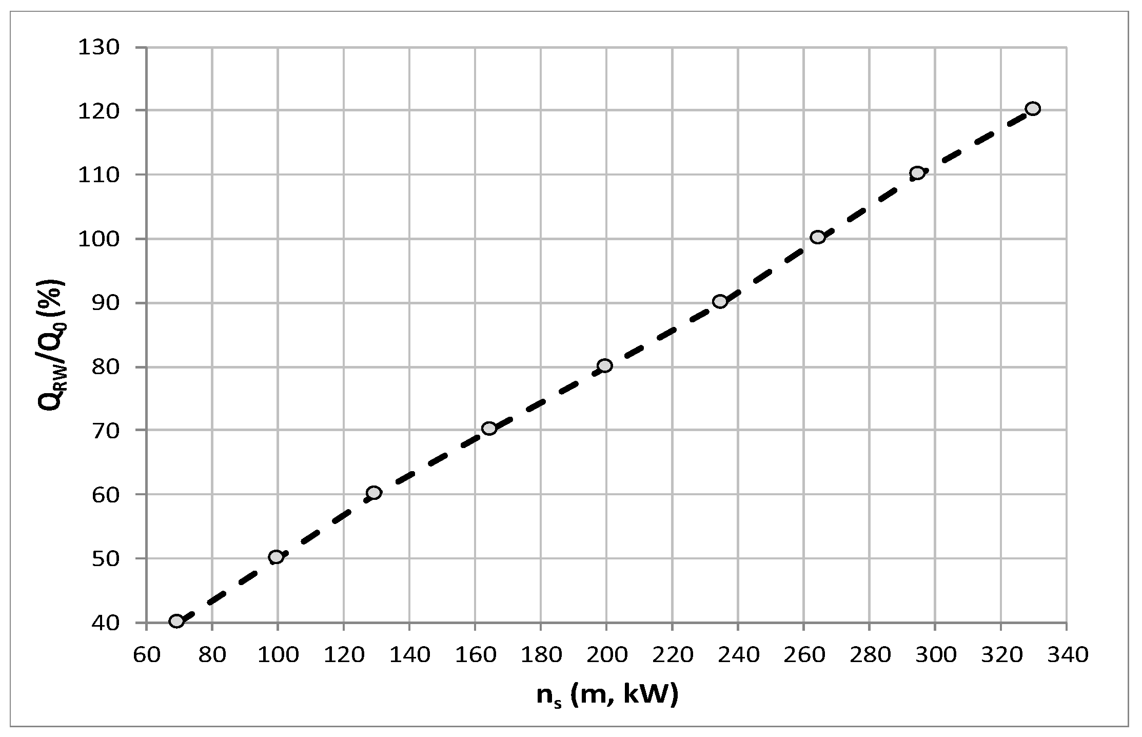
Figure 4.
Overspeed effect on the discharge variation (RW/0) of reaction turbines (adapted from [6,35]).

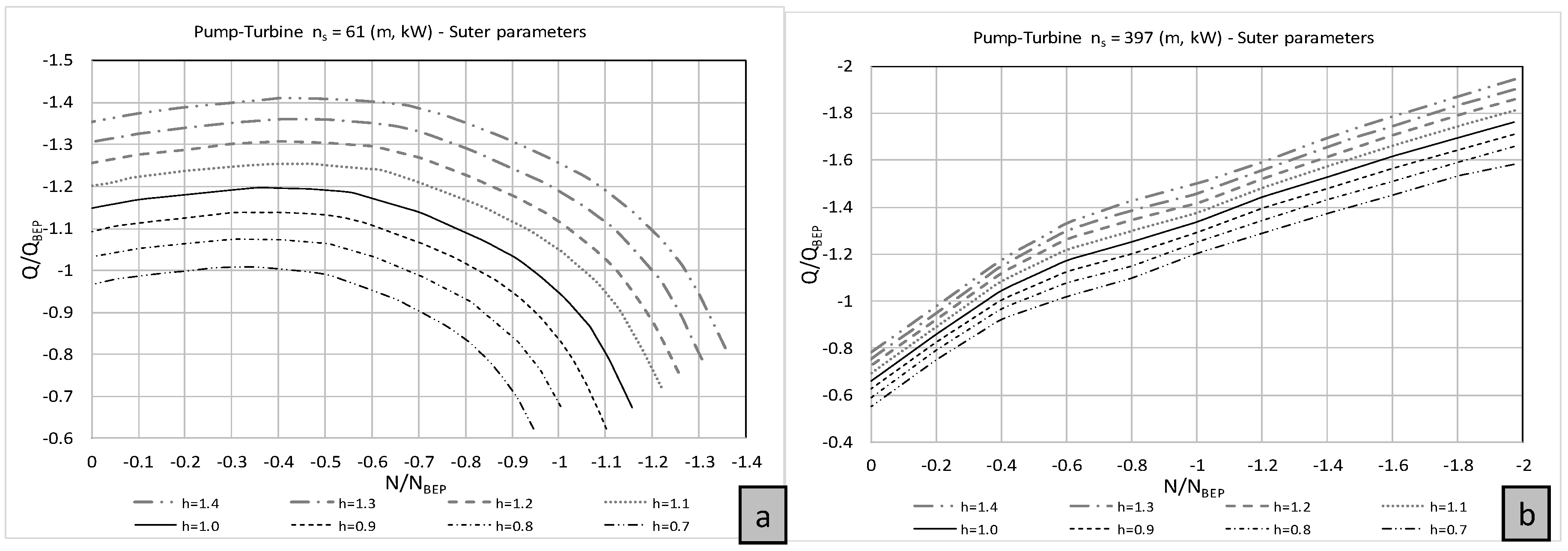
Figure 5.
/BEP as function of N/NBEP and h for (a) radial and (b) axial machine (adapted from [47,48,49]).

Figure 6.
Lab set-up. (a) experimental facility at IST; (b) scheme of the facility [6].
Figure 6.
Lab set-up. (a) experimental facility at IST; (b) scheme of the facility [6].

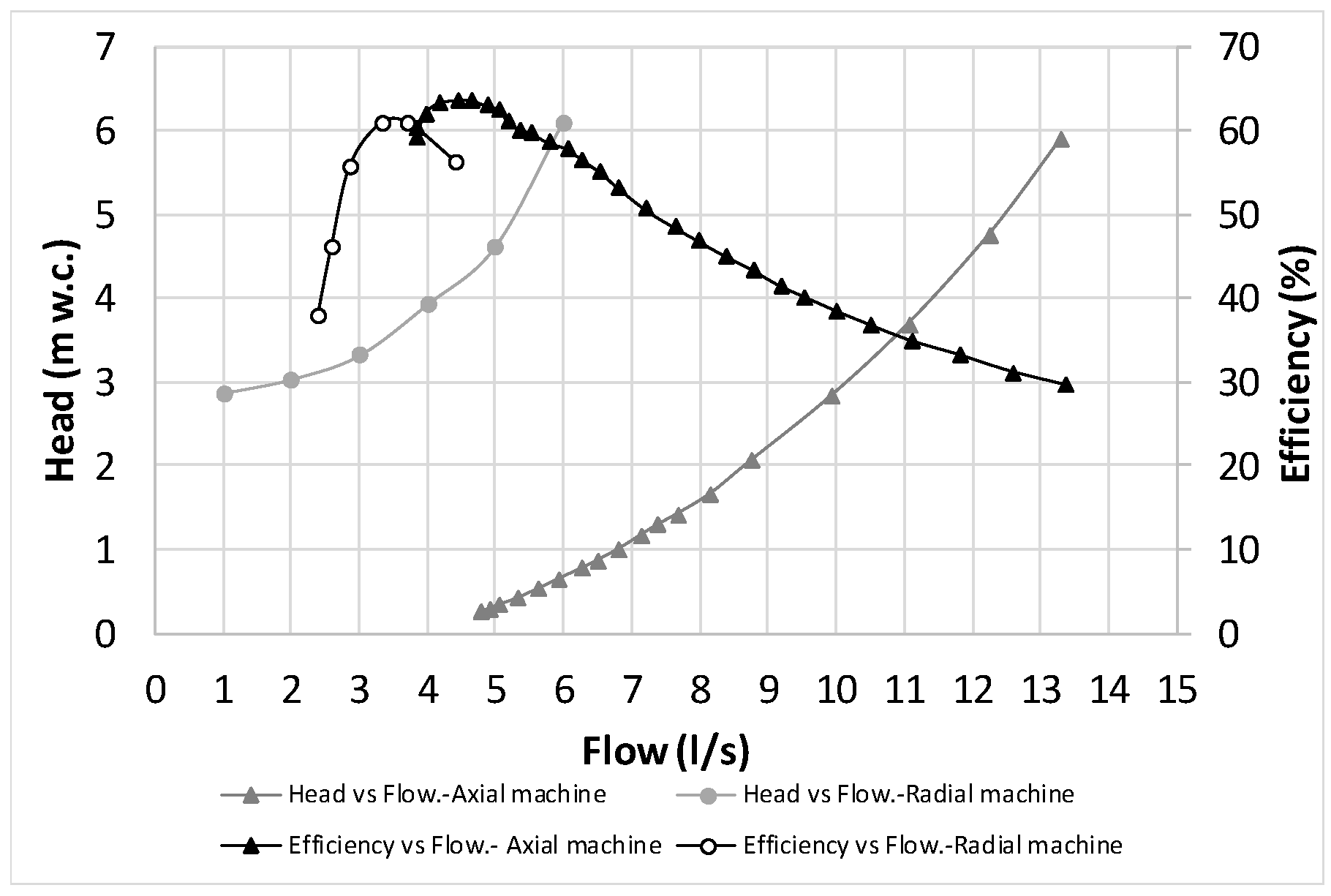
Figure 7.
Experimental Head and Efficiency curves of axial (N0 = 750 rpm) and radial (N0 = 1020 rpm) machines.
Figure 7.
Experimental Head and Efficiency curves of axial (N0 = 750 rpm) and radial (N0 = 1020 rpm) machines.

Figure 8.
Simulation scheme used in Allievi model.

Figure 9.
Experimental data recorded for the fast closure of the downstream control valve in radial and axial turbine machines. (a) flow for radial machine (b) rotational speed for radial machine (c) flow for axial machine (d) rotational speed for axial machine.
Figure 9.
Experimental data recorded for the fast closure of the downstream control valve in radial and axial turbine machines. (a) flow for radial machine (b) rotational speed for radial machine (c) flow for axial machine (d) rotational speed for axial machine.

Figure 10.
Experimental and simulated pressure values along time in a fast closure manoeuvre (t = 2 s): (a) radial and (b) axial machine.
Figure 10.
Experimental and simulated pressure values along time in a fast closure manoeuvre (t = 2 s): (a) radial and (b) axial machine.

Figure 11.
Experimental data recorded flow and rotational speed for the fast opening of the downstream control valve in turbine machines. (a) flow for radial machine (b) rotational speed for radial machine (c) flow for axial machine (d) rotational speed for axial machine.
Figure 11.
Experimental data recorded flow and rotational speed for the fast opening of the downstream control valve in turbine machines. (a) flow for radial machine (b) rotational speed for radial machine (c) flow for axial machine (d) rotational speed for axial machine.

Figure 12.
Experimental data and simulation for pressure variation due to a fast opening downstream control valve of (a) radial and (b) axial machine.
Figure 12.
Experimental data and simulation for pressure variation due to a fast opening downstream control valve of (a) radial and (b) axial machine.

Figure 13.
Experimental data of flow, rotational speed, and upstream and downstream head in the radial machine under the overspeed effect. (a) flow for radial machine (b) rotational speed for radial machine (c) flow for axial machine (d) rotational speed for axial machine.
Figure 13.
Experimental data of flow, rotational speed, and upstream and downstream head in the radial machine under the overspeed effect. (a) flow for radial machine (b) rotational speed for radial machine (c) flow for axial machine (d) rotational speed for axial machine.

Figure 14.
(a) QRW/0 and HRW/H0 as a function of NRW/N0 and (b) /BEP as a function of N/NBEP and H/HBEP for the radial machine.
Figure 14.
(a) QRW/0 and HRW/H0 as a function of NRW/N0 and (b) /BEP as a function of N/NBEP and H/HBEP for the radial machine.

Figure 15.
Experimental data of (a) flow, (b) rotational speed, and (c) the upstream and (d) downstream head in the axial machine under the overspeed effect.
Figure 15.
Experimental data of (a) flow, (b) rotational speed, and (c) the upstream and (d) downstream head in the axial machine under the overspeed effect.

Figure 16.
(a) RW/0 and HRW/H0 as a function of NRW/N0 and (b) /BEP as a function of N/NBEP and h = H/HBEP for the axial machine.
Figure 16.
(a) RW/0 and HRW/H0 as a function of NRW/N0 and (b) /BEP as a function of N/NBEP and h = H/HBEP for the axial machine.


Table 1.
Basic parameters for the simulation.
| Material | Inner Diameter (m) | Roughness (mm) | Wave Speed (m/s) |
|---|---|---|---|
| HDPE | 0.044 | 0.2 | 280 |
| PVC | 0.110 | 1.2 | 385 |
| Rigid PVC | 0.047 | 0.2 | 527 |
| Steel | 0.068 | 2 | 1345 |
© 2018 by the authors. Licensee MDPI, Basel, Switzerland. This article is an open access article distributed under the terms and conditions of the Creative Commons Attribution (CC BY) license (http://creativecommons.org/licenses/by/4.0/).
Share and Cite
MDPI and ACS Style
Pérez-Sánchez, M.; López-Jiménez, P.A.; Ramos, H.M. PATs Operating in Water Networks under Unsteady Flow Conditions: Control Valve Manoeuvre and Overspeed Effect. Water 2018, 10, 529. https://doi.org/10.3390/w10040529
AMA Style
Pérez-Sánchez M, López-Jiménez PA, Ramos HM. PATs Operating in Water Networks under Unsteady Flow Conditions: Control Valve Manoeuvre and Overspeed Effect. Water. 2018; 10(4):529. https://doi.org/10.3390/w10040529
Chicago/Turabian StylePérez-Sánchez, Modesto, P. Amparo López-Jiménez, and Helena M. Ramos. 2018. "PATs Operating in Water Networks under Unsteady Flow Conditions: Control Valve Manoeuvre and Overspeed Effect" Water 10, no. 4: 529. https://doi.org/10.3390/w10040529
Note that from the first issue of 2016, this journal uses article numbers instead of page numbers. See further details here.