Sub-Seasonal Snowpack Trends in the Rocky Mountain National Park Area, Colorado, USA
by
 , , and
Steven R. Fassnacht
1,2,3,4,* ,
,
Niah B.H. Venable
1,2 ,
,
Daniel McGrath
5 and
Glenn G. Patterson
5,6 1
ESS-Watershed Science, Colorado State University, Fort Collins, CO 80523-1476, USA
2
Natural Resources Ecology Laboratory, Colorado State University, Fort Collins, CO 80523-1499, USA
3
Cooperative Institute for Research in the Atmosphere, Colorado State University, Fort Collins, CO 80523-1375, USA
4
Cartography, GIS and Remote Sensing Department, Institute of Geography, Georg-August Universität Göttingen, Goldschmidt Street 5, 37007 Göttingen, Germany
5
Department of Geosciences, Colorado State University, Fort Collins, CO 80523-1482, USA
6
Public Health, University of Colorado Denver, Aurora, CO 80045, USA
*
Author to whom correspondence should be addressed.
Water 2018, 10(5), 562; https://doi.org/10.3390/w10050562
Submission received: 11 April 2018
/
Revised: 22 April 2018
/
Accepted: 24 April 2018
/
Published: 26 April 2018
(This article belongs to the Special Issue Effects of Climate Change on the Hydrology and Water Quality of Snow-Dominated Mountainous Environments)
Abstract
:We present a detailed study of the snowpack trends in the Rocky Mountain National Park (RMNP) using snow telemetry and snow course data at a monthly resolution. We examine the past 35 years (1981 to 2016) to explore monthly patterns over 36 locations and used some additional data to help interpret the changes. The analysis is at a finer spatial and temporal scale than previous studies that focused more on aggregate- or regional-scale changes. The trends in the first of the month’s snow water equivalent (SWE) varied more than the change in the monthly SWE, monthly precipitation or mean temperature. There was greater variability in SWE trends on the west side of the study area, and on average the declines in the west were greater. At higher elevations, there was more of a decline in the SWE. Changes in the climate were much less in winter than in summer. Per decade, the average decline in the winter precipitation was 4 mm and temperatures warmed by 0.29 °C, while the summer precipitation declined by 9 mm and temperatures rose by 0.66 °C. In general, November and March became warmer and drier, yielding a decline of the SWE on December 1st and April 1st, while December through February and May became wetter. February and May became cooler.
1. Introduction
Often referred to as “nature’s water tower” [1], snowpack of the Colorado mountains provides seasonal water storage, releasing the stored winter precipitation as melt during the spring and early summer when water demand for reservoir storage and irrigation is high [2] and other water sources are minimal. Over 60% of annual precipitation in Colorado falls as snow, with snowmelt runoff generating about 80% of the streamflow [3,4,5]. As is the case for most of the western United States, Colorado’s economy is sensitive to changes in water availability and hence to changes in both the volume of water stored in the seasonal snowpack and the rate and timing of snowmelt. One estimate of the marginal value of an acre-foot (1233 m3) of water under conditions of changing streamflow is $34–$46 in 1985 U.S. dollars [6]. This equates to $75–$102/acre-foot (6–8 cents/m3) in 2016 U.S. dollars. A difference of 1 mm in the snow water equivalent (SWE) over the 107,550 ha of the Rocky Mountain National Park (RMNP) would equate to a marginal value for water of about $77,000 per year.
In addition to providing the water supply, the seasonal snowpack is an important recreational resource. Between 2005 and 2015, the economic impact of the downhill ski industry in Colorado grew from $2.5 billion to $4.8 billion [7]. During the same period, recreational visits to the RMNP in March, a peak winter recreational-use month, more than doubled from ~60,000 to over 130,000 [8,9]. In 2011, 63% of winter visitors to the RMNP participated in recreation such as snowshoeing, cross-country skiing, sledding, and back-country skiing [10]. As for the water-supply industry, winter recreation and its associated economic benefits are sensitive to changes in the seasonal snowpack. Potential impacts on the ski industry include not only the loss of skiable snow [11], but also an increased risk of wet avalanches [12]. The difference in the annual economic value of Colorado’s ski industry in a low snow year compared with a high snow year has been estimated at $154 million [13]. Assuming that the difference in the SWE on April 1st (a common date of measure) in the snow zone in a low snow year compared with a high snow year is typically about 500 mm, then a difference of 1 mm averaged across Colorado’s snow zone would equate to a marginal value for recreation of about $308,000 statewide.
The accumulation and ablation of snow are tightly linked with temperature and precipitation. Across Colorado, a warming trend of about 0.37 °C/decade has been observed in one study [14] and in the order of 0.5–0.7 °C/decade in two other studies [15,16], although warming is not uniform throughout space and time. More rapid warming is occurring in the northern central mountains of Colorado, and cooling trends have been reported at a few stations in the southern San Juan Mountains [17,18]. Warming trends also vary with elevation, with some studies documenting more rapid warming trends at higher elevation sites [19], and others finding the fastest rates of warming at mid-elevations over longer periods (>50 year record), but with higher elevations and mid-elevations warming more equally over shorter time spans [20]. Seasonal variability in trends has also been observed, with more warming documented in the early and late winter months of November and March [18].
While the majority of station records show warming in recent decades, precipitation trends vary in space and time, reflecting not only the varying weather patterns that bring moisture to different parts of the state at different times, but also the effects of a changing climate [18]. Unlike the pervasive temperature trends, no obvious overall trends in cold-season precipitation were found in [16], although Regional Kendall test (RKT) analyses [21] indicated significant decreases in winter precipitation in 6 of 13 regional drainages, with 4 of those in the Colorado River Basin. Seasonal snowpack declined over most of the western United States over the second half of the last century [17,22]. While observed changes in Colorado have been less pronounced than in warmer maritime mountain ranges, observed changes include a reduction in the duration of snow cover over the highest elevations [16], earlier onset for snowmelt and center of mass, [15,16] and modest reductions in the SWE for the period of study. The magnitude of the reduction was dependent on whether the assessment was done on the SWE of April 1st or of the date of the maximum SWE [15,16].
Annual accumulations vary with elevation in most locations [23,24], with small declines (1–3 cm/decade) seen along the northern Front Range of Colorado [15]. Temporal variability of snow accumulation occurs on annual, seasonal, and monthly timescales and is also dependent on the period of record analyzed [25,26]. Melt rates from ablation at the end of the winter have been shown to vary [27,28]. Earlier snowmelt is generally associated with earlier spring runoff in streams [15,29,30,31], although in some parts of Colorado, trends were toward later snowmelt runoff [32].
Because of the importance of seasonal snowpack for the water supply and the winter recreation economy, a better understanding of sub-seasonal trends in snowpack accumulation and ablation is needed. Previous work analyzed characteristics of the snowpack typically using the SWE measured on April 1st as the annual peak [17,22,33,34,35,36,37,38], using the seasonal SWE [39], and using the peak SWE [15,16]. Most previous research focused on larger regions such as the Western United States or the entire Rocky Mountains, but analysis of change over smaller areas is also meaningful, especially when considering possible effects on local economies and water supplies. The objectives of this work are therefore to examine trends in snowpack accumulation and ablation across the northern Front Range of Colorado, an area within 50 km of and including the RMNP (Figure 1a), using time series of data with more than one measurement of the SWE per year. We used 35 years’ worth (1981–2015) of monthly SWE data from the manual snow course and automated Snowpack Telemetry (SNOTEL) stations to evaluate spatial trends locally and generally west and east of the Continental Divide and temporal trends on a monthly and seasonal basis. Trends in the SWE were also compared to the station elevation, precipitation and temperature, as well as the elevation of the freeze level or zero-degree isotherm.
2. Study Area and Data
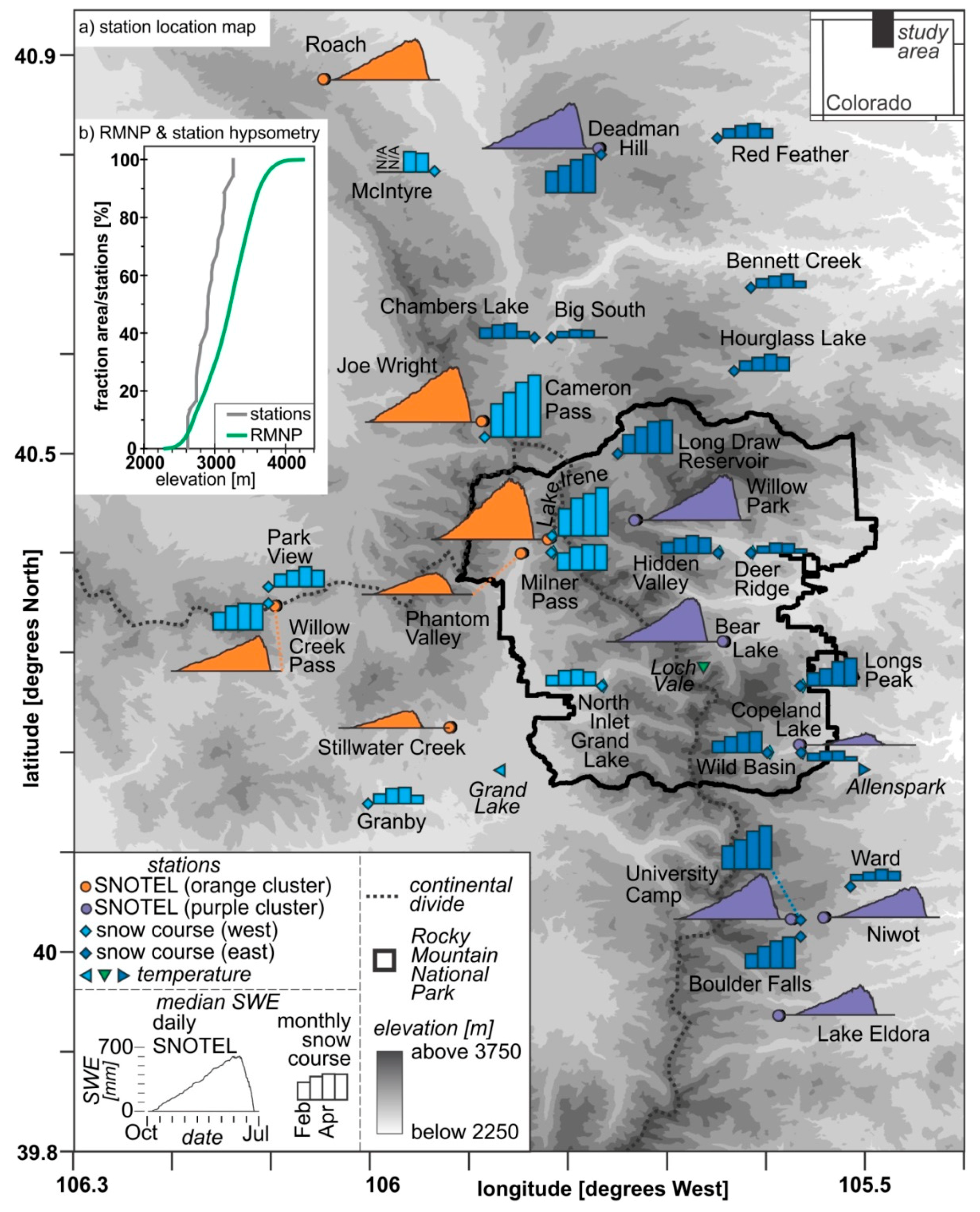
Thirty-six snow stations were used in this analysis: 13 SNOTEL stations and 23 snow courses (Figure 1a). To facilitate comparisons with previous work, we grouped these stations comparably to Clow’s [15] six clustered SNOTEL stations on the west side of the RMNP, colored orange in his work, and seven SNOTEL stations on the east side of the RMNP, colored purple; the snow courses were selected on the basis of proximity, that is, within the area of the SNOTEL stations and on the length and completeness of the records. All data are available from the U.S. Natural Resources Conservation Service (NRCS) at www.wcc.nrcs.usda.gov [40,41]. Observations were disproportionately sparse at the higher elevations of the RMNP (Figure 1b), which is common for such stations [42,43]. The RMNP extends from 2100 m up to a maximum elevation of 4346 m (Longs Peak), but approximately 1/3 of the RMNP’s hypsometry is within the alpine (>3505 m) and approximately 50% is within the sub-alpine or zone of maximum seasonal snow cover (2895–3505 m; Figure 1). Partly because of its proximity to Denver and other rapidly growing population centers along the Front Range, over 3,000,000 visitors come to the park each year [9], and over 6,000,000 recreational visits per year are made to the surrounding Arapaho–Roosevelt National Forest [44].
Snowmelt runoff from the study area contributes a large portion of the flow to the Colorado, North and South Platte Rivers [45]. The alpine areas experience a range of temperatures from about −37 to 24 °C from winter to summer, with lower elevations typically being about 5 °C warmer [9]. The total annual precipitation at Estes Park near the RMNP, at an elevation of 2293 m above sea level, is 352 mm, with some precipitation occurring in every month of the year.
The greatest amount of precipitation in terms of the percentage of annual totals occurs between May and August, with an average of about 14% occurring in any of those months [9]. About 68% of the total annual precipitation occurs from November to May, totaling about 830 mm. Precipitation is relatively evenly distributed across the calendar year, although March through May receives 34% and June through September only sees 25% of the annual total. The peak SWE in the study area ranges from 100 to 1400 mm and occurs from mid-March through mid-May (Figure 1a), depending on location, elevation, and the amount of winter precipitation [46,47].
Precipitation and temperature are measured at the SNOTEL stations. However, because changes in sensor technology have complicated the evaluation of long-term temperature trends at these stations [48], additional temperature records were obtained from three non-SNOTEL sites: Grand Lake from the National Oceanic and Atmospheric Administration [49], Loch Vale from the U.S. Geological Survey [50], and Allenspark from private monitoring by William P. Rense [51,52]. Efforts have been made to adjust the SNOTEL temperature [53,54], and the data from [55] have been used herein. Specifically, the data from after the sensor change were considered to be more homogenous across the entire SNOTEL data and were thus used as the reference [53]. For each daily mean temperature from the time series prior to the sensor change, the bias was computed using an equation derived from a set of co-located pre- and post-change sensors [53]. The pre-change data were adjusted for this bias [54,55].
The North American Freezing Level Tracker [56] was used to estimate the monthly mean elevation of freezing temperatures. This freezing level is also known as the zero-degree isotherm. The tracker simulates freezing in the free atmosphere, unaffected by terrain, and the algorithm is defined by the following: “the elevation above sea level in the free atmosphere at which a temperature of 0 °C (or 32 °F) is first encountered. The mean daily temperature profile used for this process is formed from the four six-hour averages available from Global Reanalysis” [56]. The National Centers for Environmental Prediction/ National Center for Atmospheric Research (NCEP/NCAR) Reanalysis is used [56]. The spatial discretization of the model is 2.5° × 2.5° latitude by longitude, and thus two pixels centered at 40° N latitude were used to represent the west and east sides of the study area: one at 107.5° W longitude and the other at 105° W longitude [56].
3. Methods
We assessed spatial and temporal variability in the SWE over this 35 year interval (1981–2015) using monthly records of the SWE at 23 snow courses. SWE observations were made at each snow course on approximately the first day of each month from February to May (except McIntyre, which only had measurements in April and May) [57]. In addition, we utilized the first of the month’s (November to June) daily SWE observations from 13 SNOTEL stations. The first of the month’s SWE data were also used to compute the monthly change in the SWE. Daily SNOTEL data were used to compute the monthly cumulative precipitation and mean temperature as well as seasonal means and totals; an average winter value was calculated over the November to May period, and an average summer value was calculated over the June to September period. The mean monthly and seasonal temperatures were computed for the three non-SNOTEL meteorological stations.
Trend analyses were performed on all monthly and seasonal data using the Mann–Kendall test for the monotonic trend [58,59,60] to determine the significance of trends and the Theil–Sen estimate of the slope of the linear trend [60,61,62,63]. Two significance levels were applied, with confidence levels of p < 0.05 (called significant) and p < 0.10 (called moderately significant). Rates of change were calculated for each snow course and SNOTEL station and for groupings of west versus east stations and courses. Rates were also calculated for the non-SNOTEL temperature monitoring meteorological stations and for the modeled freezing level or zero-degree isotherm. Trends in the monthly SWE, precipitation and temperature for all stations were correlated with elevation. The correlation coefficient, the change in trend per unit of elevation, and the y-intercept of the best-fit linear function were computed. The monthly and seasonal precipitation and temperature trend data were also correlated with one another and with changes in the SWE.
4. Results
4.1. First of the Month’s SWE Trends
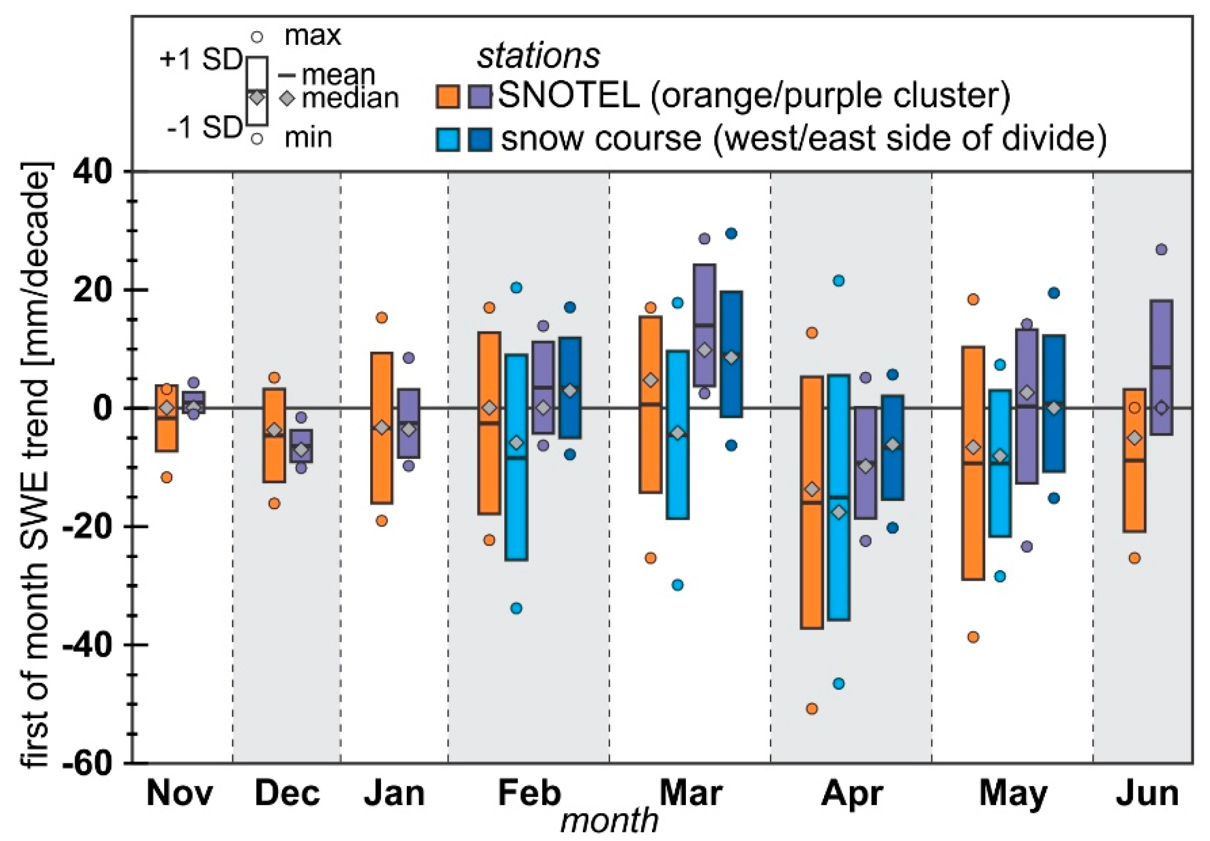
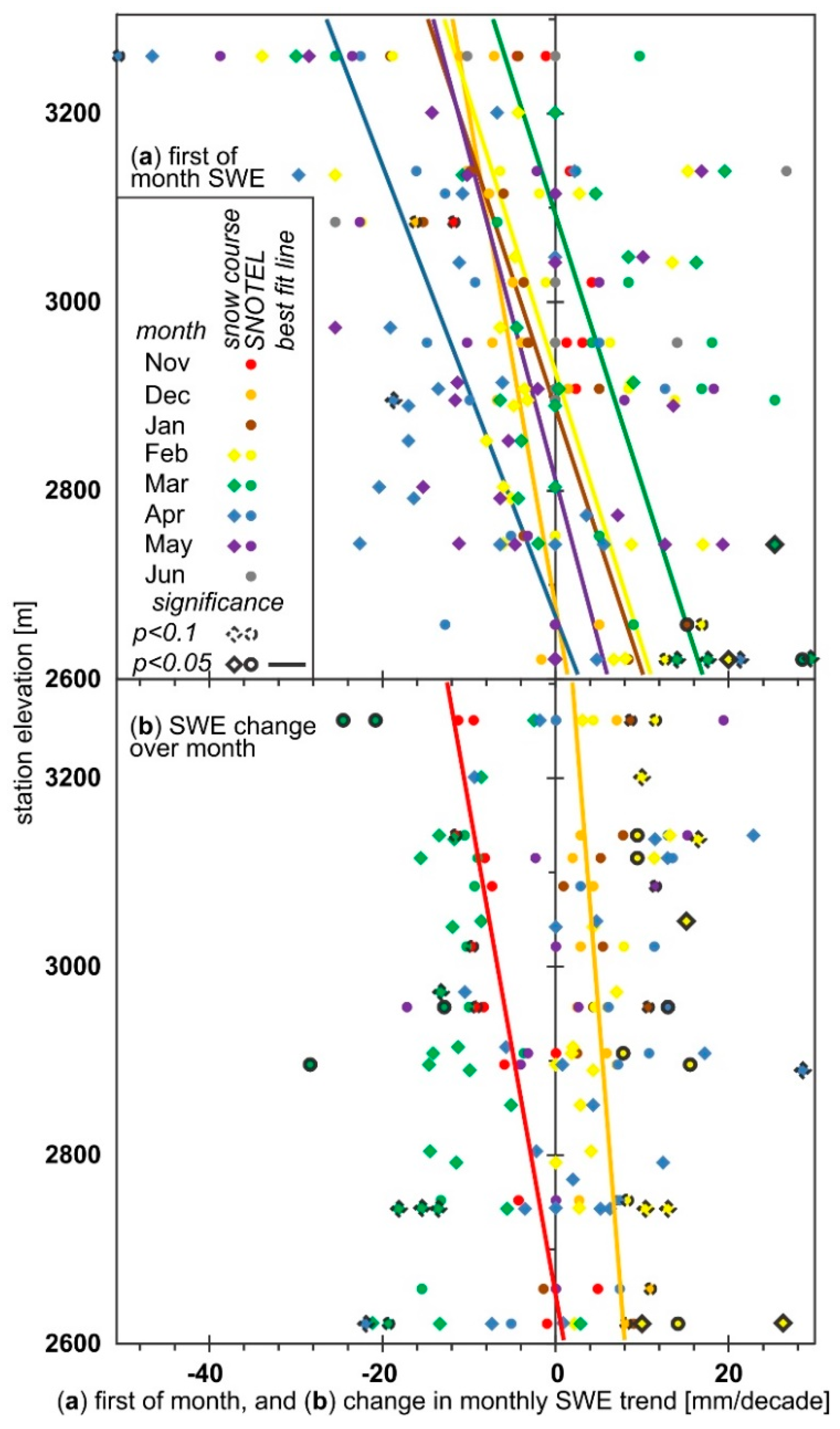
On the standard measurement date of April 1st, the SWE decreased at 25 of the 36 locations. The median decrease was 10.9 mm/decade. No change was found at four locations, all of which were on the eastern side of the Continental Divide (Figure 2, Figure 3 and Figure 4). At two locations (Lake Irene SNOTEL station and Ward snow course), the decreases were only moderately significant (p < 0.10), and there was a moderately significant increase at the Granby snow course (Figure 3a). The April 1st SWE trends varied spatially (blue bars in Figure 4), with greater variability in trends on the west compared to the east, particularly in the months of February, March and April (orange and light blue versus purple and dark blue in Figure 2 and Figure 3).
Although the April 1st SWE trends were primarily negative, this pattern was not temporally consistent (Figure 2, Figure 3 and Figure 4). We found that most stations also exhibited decreasing SWE trends on November 1st and December 1st, but increasing trends on March 1st (Figure 2). Generally speaking, western stations exhibited either a greater reduction in the SWE or a smaller increase than stations to the east of the Continental Divide (Figure 2).
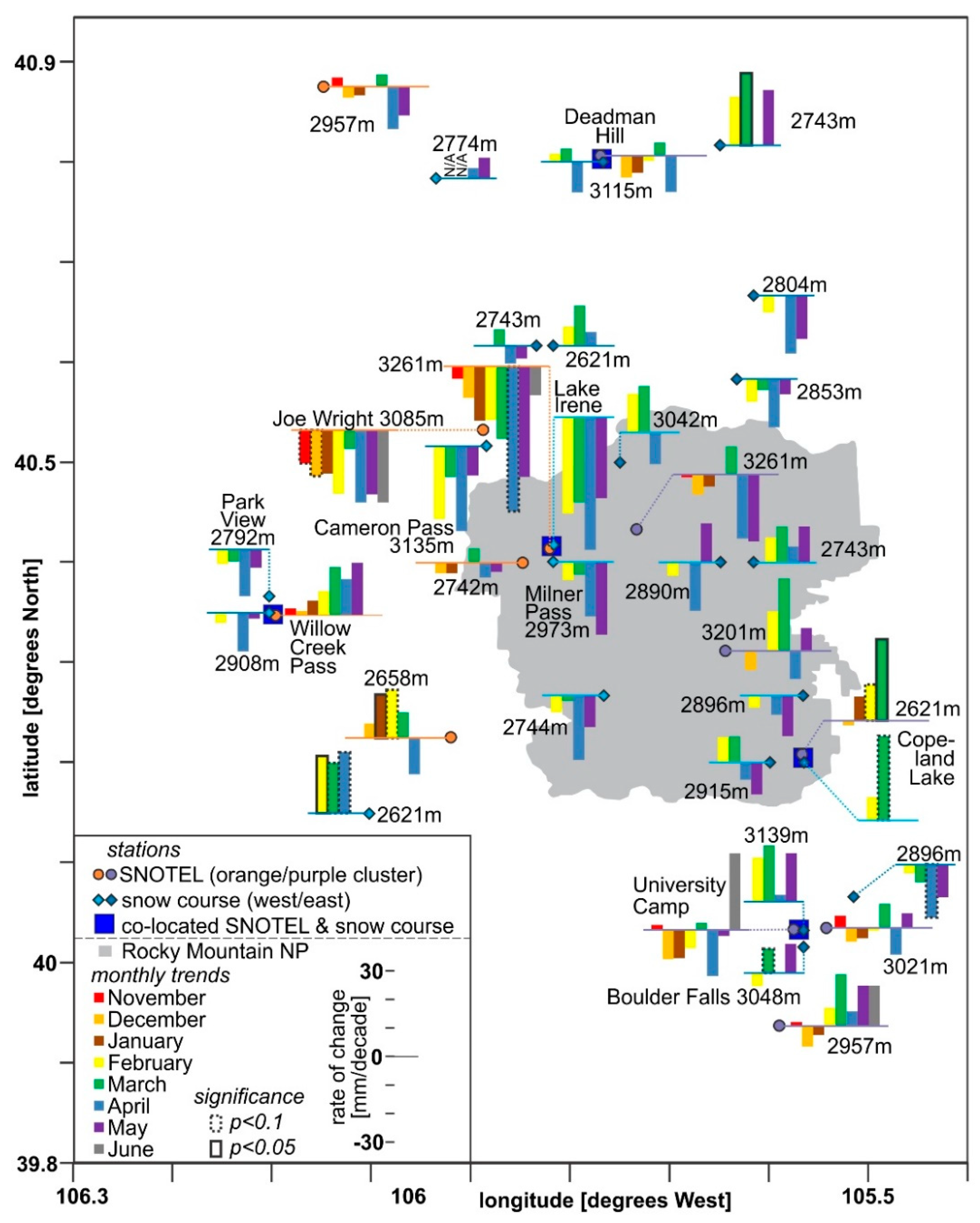
As would be expected, there was a high degree of spatial auto-correlation between most measurement sites. Stations in close proximity to one another generally had similar trends, such as for the Joe Wright SNOTEL and Cameron Pass snow course, the Park View and Willow Creek Pass snow courses, the Lake Irene and Milner Pass snow courses, and the Boulder Falls and University Camp snow courses (labeled in Figure 4). There were similar trends among three co-located SNOTEL and snow course stations, specifically Lake Irene, Copeland Lake, and Deadman Hill, but opposite trends at two other co-located measurement sites, specifically Willow Creek Pass and University Camp (labeled as co-located in Figure 4).
There was a significant correlation between the first of the month’s SWE trends and elevation for the months of December through May, with r2 values ranging from a low of 0.16 for May to a high of 0.66 in January (Figure 5a; Table 1a). With an increase in elevation, the decrease in the SWE trend became greater, that is, the slope was negative (Table 1a). From the best-fit line, the y-intercept changed from 2676 m in December to 3093 m in March and then lowered again; above this elevation SWE trends were decreasing and below they were increasing. The slope of the relation between the SWE trend and elevation was similar for all months except December, when the rate of change was about half, and for November and June, when the trend was not significant (Figure 5a; Table 1a).
4.2. SWE Trends over the Month
Trends in the SWE change over the month (Figure 6a) were more consistent between station and course clusters than the first of the month’s SWE trends (Figure 2). Over the months of November and March, there was a decrease in the change in the monthly SWE at all stations and snow courses, with the exception of two stations in the west group, with increases in November, and one station also in the west, with an increase in the SWE in March (Figure 3b). Conversely, from December through February, there was an increase at all stations and snow courses, except one station in the west, which decreased in January, and one snow course in the eastern group that had no change in February (Figure 3b).
The change in the SWE over the month was only significantly correlated to elevation in November and December (Figure 3b and Figure 5b); the correlation was similar to the first of the month’s SWE, as there was a decrease with increased elevation (Figure 5b). Over the month of May, the change in monthly SWE trends increased greatly with elevation, but not significantly (Figure 5b).
4.3. Precipitation, Temperature and Freezing-Level Trends
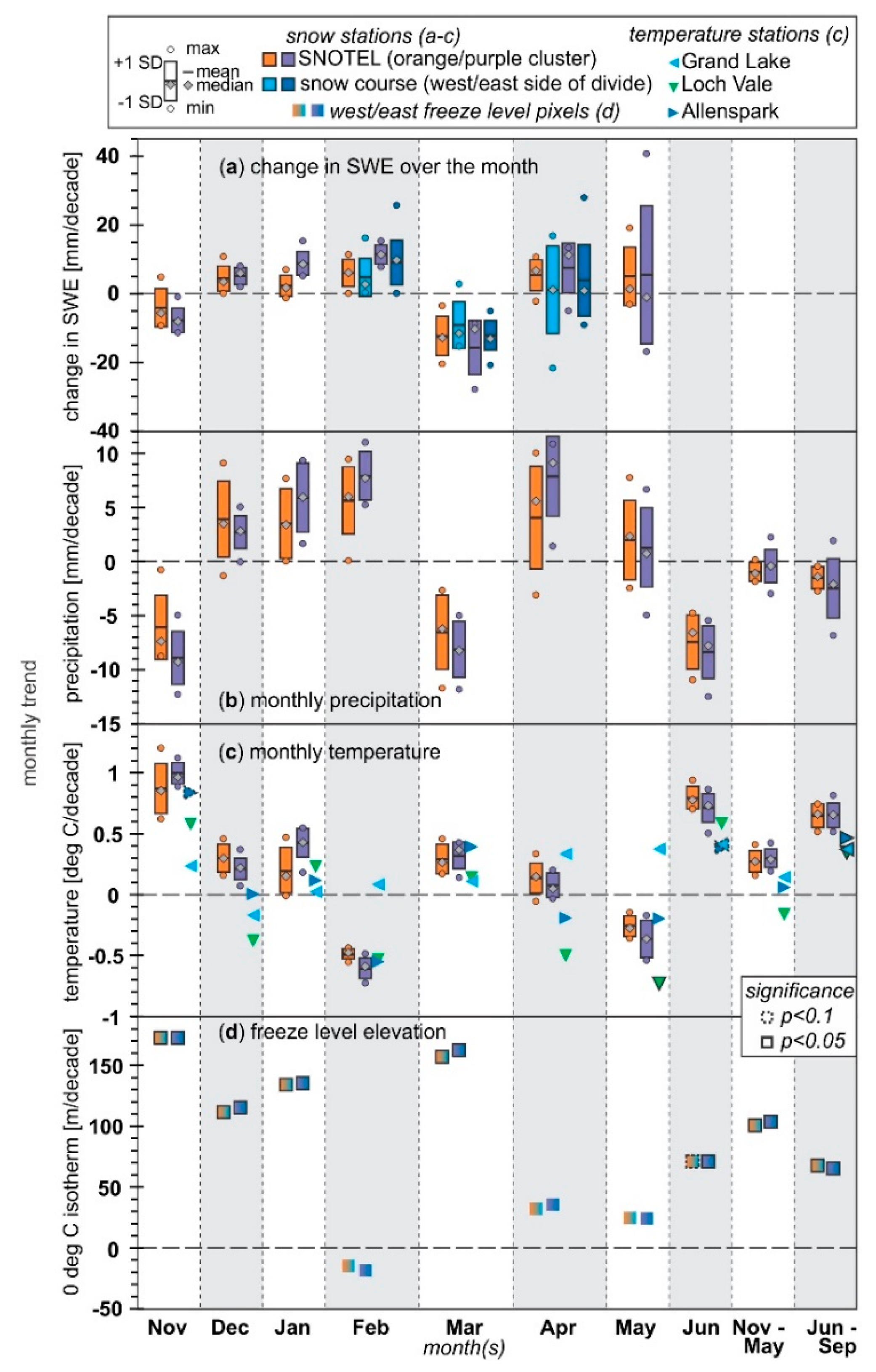
Precipitation trends mirrored changes in the SWE over the monthly trends (Figure 5b), but displayed a greater range of variability, particularly for November through February. While most (11 of 13) stations saw a decreasing trend in winter (November through May) precipitation, none were significant (Figure 3c), and all were small (results not shown). Summer (June through September) precipitation decreasing trends were greater than those in the winter (results not shown), but only one station on the east side of the divide saw a significant decrease (Figure 3c). Precipitation trends increased significantly with elevation in January and February, but decreased significantly with elevation in March, May, and throughout the summer (Table 1c).
Monthly temperatures warmed in most months at nearly all of the stations (Figure 3d and Figure 6c). However, 1 station on the west side was cooling in January, 4 of the 13 SNOTEL stations were cooling in April (1 in the west and 3 in the east), and all stations were cooling in February and May (Figure 3d and Figure 6c). All stations (Table 1d) including the independent temperature stations (Figure 6c) saw significant warming in the summer, and one station on the west side had significant warming in the winter (Table 1d). The independent temperature stations tended to have a lower-magnitude warming trend than the SNOTEL stations; the Grand Lake station exhibited a warming trend in February, April and May, while Loch Vale and Allenspark had cooling trends during those months (Figure 6c). Only the December and February monthly temperature trends were significantly correlated with elevation, and both were decreasing (Table 1d). The freeze-level elevation-change trends were increasing in all months except February (Figure 6d). The increases were significant in most months except April and May.
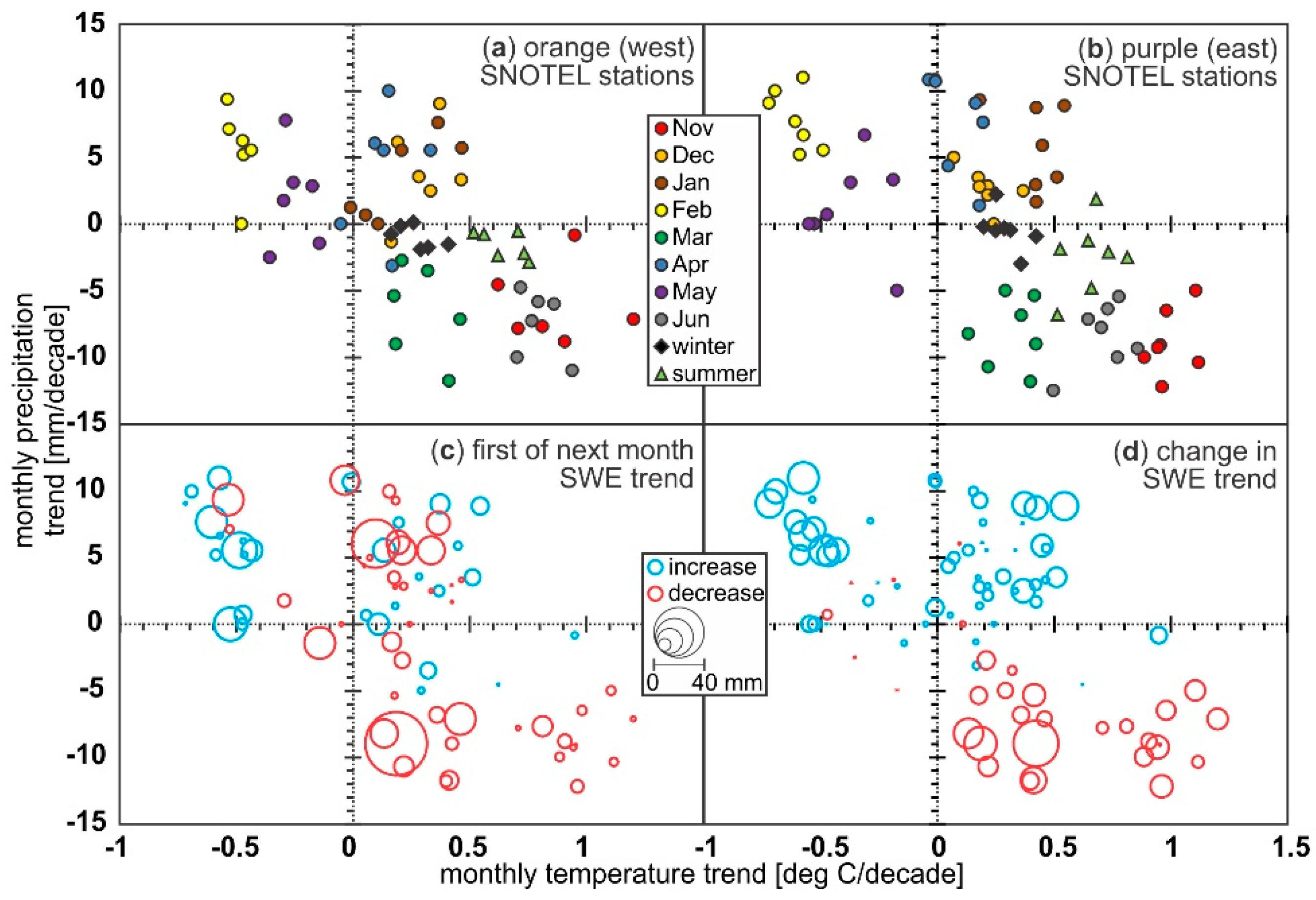
February and May were trending to be both cooler and wetter at most stations (Figure 6b and Figure 7a). November, March and June were warmer and drier, while December, January and April were warmer and wetter (Figure 7a,b). Winter trends in both the east and west station clusters were generally warmer, but with little to no trend in precipitation. Summers, however, were both warmer and drier overall (Figure 7a,b).
Because of cooler and wetter weather in February, the March 1st SWE trend was the only date that had increases in the SWE (blue circles in upper left of Figure 7c, with circle size indicating amount of increase or decrease). Changes in the SWE over the month correlated well with the monthly precipitation, with a coefficient of determination between the two variables of 0.62 (Figure 7d). There were several decreasing trends in the change in the SWE over the month when correlated with precipitation and temperature (red circles above the 0 mm/decade precipitation line in Figure 7d); most of these occurred in April or May during the melt season.
5. Discussion
5.1. Variability in Monthly Measures of SWE
Snow varies spatially (Figure 1) [2] from a fine resolution (meters) [28,64,65] to a moderate resolution (kilometers) [66] to a coarse resolution (tens to hundreds of kilometers) [23], and also varies temporally (Figure 2, Figure 3 and Figure 4) [26,39], with different climatic forcing mechanisms controlling snowpack accumulation and ablation at different times of the snow season [67].
The study domain covered complex mountainous terrain with a station density of one snow station per 200 km2 (Figure 1a). This work reveals widely varying trends from month to month (Figure 2) across all 36 stations (Figure 4), suggesting that there is a need to study finer-scale spatial trends when considering how smaller basins will respond to changes in the water supply. Even in relatively homogeneous terrain, such as the Northern Great Plains, there can be great spatial variability in climate and snow trends [66]. For the period from 1991 to 2005, the study’s SNOTEL stations (Figure 1) had three different snow climatologies, where Phantom Valley and Lake Eldora were grouped together, while Stillwater Creek and Copeland Lake were grouped together; the remaining nine stations were in the same climate grouping [24].
Temporal evaluation of trends requires a distinction between inter-annual variability and long-term trends [68,69]. Time series shorter than 15 years were found to produce inaccurate estimates of temperature trends [70], and precipitation in the western United States is often said to vary according to the double sunspot cycle, which has a period of about 22 years [71,72]. As temperature and precipitation are the primary factors that influence accumulation and ablation of the seasonal snowpack in the western United States [35], snowpack trends should also be based on time series that exceed these minimum durations. This analysis used 35 years (1981–2015) of snowpack (Figure 2, Figure 3, Figure 4, Figure 5 and Figure 6), precipitation (Figure 6b), temperature (Figure 6c), and freezing-level elevation (Figure 6d). The length of records may be relevant. Declining April 1st SWE trends across the western United States have generally been attributed to widespread long-term warming, but not to shorter-length cyclical climate variability patterns, such as Pacific Decadal Oscillation [35].
Here we present spatio-temporal trends at a moderate spatial resolution over a 35 year period of record (Figure 2, Figure 3, Figure 4 and Figure 5) and show that trends tend to vary more on the basis of the time of year (month) than the location (elevation or west–east). However, there tended to be greater decreases and a greater variation in the first of the month’s SWE on a monthly basis for snow stations west of the Continental Divide compared to stations to the east (Figure 2). This was mirrored for changes in the SWE over the month (Figure 6a) and monthly precipitation (Figure 6b). These spatio-temporal changes were observed in previous studies, but they were only resolved at a coarse resolution (e.g., [34,39]), not at the scale of smaller watersheds or basins, and not on a time step that may be relevant for seasonally snow-dependent economic activities such as winter recreation [11,13].
In the study area, decreasing trends for the April 1st SWE in the range of 12–27 mm/decade [15,16] were previously found using the RKT [21]. Here we used the Mann–Kendall test and Theil–Sen’s slope, resulting in a mean decrease overall of 10.7 mm/decade, with a range in values from an increasing trend of 21.4 mm/decade to a decrease of 50.8 mm/decade (Figure 2). To the west of the divide, three stations had an increasing April 1st SWE trend, and on the east, four stations were increasing (Figure 3a); these stations’ elevations (2621 m at Granby and Big South to 3139 m at University Camp; Figure 2) spanned over most of the range of station elevations (Figure 1b).
Changes in the SWE over the month can be used as an indicator of conditions leading up to the next first of the month’s SWE measurement (Figure 6a), dictating the amount of snow at the beginning of the next month (Figure 2). However, only 48% of the station months analyzed had month-to-month trends occurring in the same direction (either both decreasing, or both increasing; Table 1a vs. 1b), with a coefficient of determination between the trends of only 0.29.
Our results show that the largest decrease in the first of the month’s SWE was for April 1st (Figure 2), as is evident in the change in the SWE from March 1st to April 1st (Figure 6a). The negative shift in March’s monthly change in the SWE (less accumulation or more ablation or both) was more pronounced than the trend in the April 1st SWE. Because more SWE accumulated during February (Figure 6a) and less was still present on April 1st, the change in the SWE between March 1st and April 1st was accentuated. The change in SWE over the month of November also decreased at most stations (Figure 6b), yielding a decrease in the December 1st SWE at most stations (Figure 2). Our findings suggest that the months near the beginning (November) and end (March) of the core snow accumulation season are times that see the greatest shift toward less accumulation (November; and greatest warming—Figure 5c) and/or more ablation (March), which have implications for snow-dependent water resources and economically important recreational activities. Most ski resorts open in November and close in April; lower snow accumulations and/or greater losses or lack of gains from warming in the season’s start-up and ending months will negatively impact the industry.
5.2. Precipitation Trends
In November and March, decreasing precipitation and increasing temperatures (Figure 6) combined to reduce the SWE accumulation (Figure 2), while in February and May, the reverse was true, resulting in positive trends in the SWE change (Figure 6a). The pattern of monthly trends in precipitation explained the observed trends in the SWE, but the magnitude of the precipitation trends in this study, in the order of 10 mm/decade, were small compared with trends observed in other parts of the western United States, which exceeded 30 mm/decade [34,36]. Our study is consistent with others that found little change in precipitation in this part of northern Colorado [14,18,35].
It can be difficult to determine the phase of precipitation, that is, rain or snow, on a particular day in the snow zone [73]. Temperature records have been used to make this determination, but the temperature threshold to differentiate between the precipitation phases is not always constant [74,75]. Thus, SNOTEL station data can be used to assess the precipitation phase at high-elevation locations. Because of the winter temperatures in northern Colorado, November and April are the only months in which the warming temperatures could cause precipitation to fall as rain instead of snow [74]. However, the Colorado Rockies are generally considered to be sufficiently cold enough for the snow-to-rain fraction to be minimally affected by recent warming trends [67].
Precipitation trends tended to match changes in the SWE over the month (r2 = 0.62). Non-significant increases in winter precipitation were found in [67], while no significant trend in the ratio of the April 1st SWE to winter precipitation was found in [15], either for the west or east station groupings. Although this ratio was not examined in the present work, monthly variability in precipitation was substantial, with increases from December to February and decreases in November and March (Figure 6b). However, there was only a small, non-significant decrease in winter precipitation (Figure 3).
5.3. Temperature Trends
Over the 1981–2015 interval, this study found that winter temperatures warmed by 0.29 °C/decade, in corroboration with previous studies [19,20,35,67]. However, this overall winter warming trend confounded two conflicting monthly trends (cooling in February and May) and warming for all other winter months by 0.2 to 0.8 °C/decade (Figure 6c). A previous analysis by [15] showed no significant temperature trends in February and May and even greater warming during the other winter months (0.7 to 1.5 °C/decade increase in those months). Significant winter warming averaging about 1 °C/decade across most stations in the Upper Colorado River Basin has been found [16], while the strongest warming was found by [76] in the spring. The greater warming presented by [15,16] was due in part to sensor changes at the SNOTEL stations. During the early to mid-2000s, the SNOTEL program switched to an extended-range temperature sensor, installed a new radiation shield, instituted a new data collection protocol, and moved all temperature sensors to a new location above the snow pillow, resulting in uncertainty in record consistency over the long term [48,53]. As such, we used the SNOTEL data adjustment presented by [54] for these analyses.
For all months except January, the temperature trends decrease dwith elevation (only December and February were significant; Table 1d), and the SWE decreased with elevation (Figure 5). This suggests that the predominance of negative trends in the SWE at higher-elevation sites may be related to less accumulation rather than temperature-induced melt from warming at higher elevations (e.g., [17]). The northern Colorado Rockies are less susceptible to temperature-induced negative SWE trends than other mountainous areas in the western United States [77]. An increase in sublimation [16] can reduce the net amount of snow, especially at higher elevations. Modeled total sublimation varied from 50 to 500 mm depending on the location and wind conditions, and varied inter-annually from 149 to 260 mm across the study domain [45]. However, wind speeds have not significantly changed across northern Colorado [78].
Previous research has found elevation-dependent warming [79]. Using station data, the strongest warming trends were for maximum temperatures of 0.85 °C/decade at a mid-elevation of 2591 m, while the greatest warming was for minimum temperatures of 0.5 °C/decade at a higher elevation of 3048 m [20]. From the Parameter-elevation Regressions on Independent Slopes Model (PRISM) dataset, warming trends increased with elevation, with a mean annual warming of 0.3 °C/decade at 1500 m increasing to 0.7 °C/decade at 3500 m and finally to 0.96 °C/decade at 4000 m [19]. The issues with the SNOTEL temperature sensors [48] were not incorporated in the previous trend analyses; the trends presented herein (Figure 3d and Figure 6c) used one adjustment to the time series [54].
Using the temperature records from the SNOTEL stations (Figure 6d) preserved the association with the other data collected at the same stations, notably the SWE (Figure 2, Figure 3a and Figure 7c) and precipitation (Figure 6b). These were used to analyze trends in the first of the month’s SWE and the monthly change in the SWE in relation to trends in temperature and precipitation (Figure 7). The overall range of the three variables in this study area was less than the variability reported for the same variables in the Pacific Northwest [34].
5.4. Climatic and Other Influences on SWE
There could be more ablation in warmer months, yielding less SWE (Figure 7d), especially during November and March [17,35]. However, the December 1st and April 1st SWEs were mostly decreasing at higher elevation sites (Figure 5a) that were still too cold to melt. There was little decrease in winter (November through May) precipitation (Figure 6b), and thus the change was the timing of snowfall and possibly ablation mechanisms [16]. While there was a shift from snow to rain widespread over much of western North America and even for parts of Colorado, no such shift was observed for the northern Colorado Front Range [66].
A mechanism that could account for the warming and less SWE during November and March is albedo-feedback warming [76,79,80]. This process tends to occur near the zero-degree isotherm, which is in the vicinity of the SNOTEL sites during November and March. While the trends in the elevation of the freeze level (Figure 6d) were similar to the temperature trends (Figure 6c), it is unclear whether the computation of the zero-degree isotherm used the SNOTEL data and considered the temperature-sensor change [48].
The high, cold mountains of the northern Front Range are cold enough to support a strong snow accumulation season in December through February, but warming and SWE loss could be occurring during November and March from a loss of albedo due to snow cover losses, which in effect shortens the snow accumulation season. The decreased albedo could also be due to dust on snow at higher elevations [14,76,81] or the deposition of black carbon on snow [82]. While dust on snow has been seen in this area [83], it is usually limited in amount, as the dust source of the Four Corners area is distant [84]. Another elevation-dependent warming mechanism is positive feedback related to increased humidity that yields more downward longwave radiation; this has been found to be significant in Colorado [85].
5.5. Concerns with the Data
In addition to temperature-data issues, there may be concerns with the data used in the analysis. For example, manual measurements are often taken at snow-course locations prior to the first of the month [57]; here, April 1st snow-course measurements were made on average 3.5 days earlier across the study area: 4.2 days earlier on the west and 3.1 days earlier on the east. However, the measurements tended to be consistently early for any particular station; thus the trends were stable. Still, the early snow-course measurements could have yielded different measurements than those taken on the first of the month [86], which could be relevant when comparing to the actual first of the month’s SNOTEL measurements. This may not account for differences in trends between co-located snow-course and SNOTEL stations [46], because where co-located snow-course and SNOTEL stations were very similar (i.e., Phantom Valley, Joe Wright and Willow Park), they were discontinued [3]. Monthly trends were quite different between two sets of co-located snow-course–SNOTEL stations (Willow Creek Pass and University Camp). This illustrated spatial differences over small distances and possibly the difference in the scale of measurement [26,87].
5.6. Implications for Water and Snow Resource Management
Our findings have management implications for the water supply, wildfire, ecological resources, and winter recreation. The RMNP and its vicinity are undergoing climatic changes that are altering patterns of accumulation and ablation of the snowpack (Figure 4). However, this area is experiencing less variability in temperature, precipitation, and SWE trends than many other parts of the western United States [33,34,35,38,67].
While December through February showed increased precipitation (Figure 3c and Figure 6b) and SWE (Figure 2, Figure 3a and Figure 7c), November and March had warming and drying trends that reduced SWE accumulation at the beginning of the snow season and later in the winter (Figure 2). In terms of the water supply across the study area, winter precipitation decreased slightly (Figure 6b), while summer precipitation decreased significantly (Figure 3c). However, trends toward less accumulation or greater loss of SWE during March resulted in less SWE in the snowpack on April 1st, and variable warming trends later in the spring could enhance snowmelt and create greater uncertainty regarding water supplies during the crucial spring runoff period. If the snowpack melts earlier, this could reduce both soil moisture and streamflow [81], increase stress on vegetation, and lead to increased risk of wildfires during longer, drier summers [88]. Water managers could have less reliable water storage as snow and may need to rely more on artificial storage projects, although trends toward a wetter April and a cooler and wetter May with more snow at lower elevations (Figure 5a) may help offset these issues.
Snow-based recreation could be affected by changes in snow accumulation by concentrating the season to months with more dependable SWE accumulation, in particular, December through February (Figure 2). Less snow in November could delay the start of the ski/snowboard [12] and snowmobile seasons [89]. Recreation is also likely to become more concentrated at higher elevations, where the snow is more dependable. Variable conditions during the spring may result in an increased danger of avalanches [12]. March is the month of spring break for many students, increasing winter recreation that month [8], but a decrease of snow in March could force a quicker end to the recreation season, decreasing late winter tourism and the associated income for many tourism-dependent communities and businesses [11,90,91].
6. Conclusions
The snowpack in the RMNP and its vicinity has changed over the 35 year period from 1981 to 2015. However, few of the trends analyzed were statistically significant. Regional analyses of trends do not illustrate spatial variability in SWE trends over smaller scales. They also mask extreme values and values of opposite direction, that is, when both increasing and decreasing trends were observed over a short time period. Sub-seasonal patterns of trends in the SWE showed variations according to the date within the snow season; specifically, the temporal or month-to-month variability in SWE trends was greater than the spatial variability. On the west side of the study area, the trend was for less snow on average, but there was also greater variability in this area than on the east side of the study area. There was an inverse relation between the SWE trend and elevation; the SWE tended to decrease more at a higher elevation.
Changes in monthly SWE trends mimicked precipitation trends and were less variable than the first of the month’s SWE trends. All monthly temperatures were warming, except in February and May. The winter was drier overall by 0.7 mm/decade and warmed by about 0.3 °C/decade, but neither trend was significant. The summers warmed significantly at 0.65 °C/decade and dried 3 times as much as in the winter. November and March are warmer and drier, December and January are warmer and wetter, February and May are cooler and wetter, and April is mixed with being mostly warmer and mostly wetter.
These findings suggest that the core winter months of December, January and February have seen a constant or even enhanced trends in the SWE. However, the snow season begins with less snow because of continued warming and drying trends in November. March contributed more than 10% of the annual precipitation and yet was shown to have less snow accumulation over time, and possibly some loss of the SWE. April and May are becoming wetter, contributing almost a quarter of the annual precipitation. These results suggest a shift in the timing of precipitation and snow accumulation. Warming in April combined with that observed in summer months can cause more rapid spring snowmelt and soil moisture declines, contributing to decreased streamflow, stress on vegetation, and increased fire danger. Winter recreation could become more concentrated during the core accumulation seasons of December, January and February, while downstream water users may need to rely more on stored water to offset changes in snowmelt runoff.
Data Availability
All NRCS snow-course and SNOTEL data are available online through the Water and Climate Center at www.wcc.nrcs.usda.gov. The Grand Lake data are available online through the National Weather Service at www.ncdc.noaa.gov. The Loch Vale meteorological data were provided by the U.S. Geological Survey’s Water, Energy, and Biogeochemical Budgets (WEBB) program, and are available online through the Colorado State University at www2.nrel.colostate.edu/projects/lvws. The Allenspark station is privately monitored by William P. Rense. The digital elevation model data are available through the U.S. Geological Survey at nationalmap.gov.
Author Contributions
S.R.F. and G.G.P. conceived the original design of the work. S.R.F., D.M. and N.B.H.V. outlined the paper. S.R.F. and N.B.H.V. wrote the paper, with input from D.M. G.G.P. obtained the non-SNOTEL temperature datasets. S.R.F. collated and analyzed all of the data and created all the tables and figures. N.B.H.V., G.G.P. and D.M. provided comments on the figures.
Funding
This research was funded by the National Park Service Continental Divide Science and Learning Center of the Rocky Mountain National Park agreement number P12AC10943, and through the National Park Service Water Resources Division Task agreement number P16AC00826.
Acknowledgments
Thanks are given to Amanda N. Weber for her early input to this work. We thank Professor William Rense, who provided his personal data from the Allenspark meteorological station.
Conflicts of Interest
The authors declare no conflict of interest.
References
- Viviroli, D.; Dürr, H.H.; Messerli, B.; Meybeck, M.; Weingartner, R. Mountains of the world, water towers for humanity: Typology, mapping, and global significance. Water Resour. Res. 2007, 43, W07447. [Google Scholar] [CrossRef]
- Bales, R.C.; Molotch, N.P.; Painter, T.H.; Dettinger, M.D.; Rice, R.; Dozier, J. Mountain hydrology of the western United States. Water Resour. Res. 2006, 42, W08432. [Google Scholar] [CrossRef]
- Serreze, M.C.; Clark, M.P.; Armstrong, R.L.; McGinnis, D.A.; Pulwarty, R.S. Characteristics of the Western United States snowpack from snowpack telemetry (SNOTEL) data. Water Resour. Res. 1999, 35, 2145–2160. [Google Scholar] [CrossRef]
- Barnett, T.P.; Pierce, D.W.; Hidalgo, H.G.; Bonfils, C.; Santer, B.D.; Das, T.; Bala, G.; Wood, A.W.; Nozawa, T.; Mirin, A.A.; et al. Human-induced changes in the hydrology of the western United States. Science 2008, 319, 1080–1083. [Google Scholar] [CrossRef] [PubMed]
- Colorado Climate Center. Colorado Climate Center; Colorado State University: Fort Collins, CO, USA; Available online: http://climate.colostate.edu/ (accessed on 10 April 2018).
- Harding, B.L.; Payton, E.A. Marginal economic value of streamflow. Water Resour. Res. 1990, 26, 2845–2859. [Google Scholar]
- RRC Associates. Colorado Ski Country USA: Economic Study Reveals Ski Industry’s $4.8 Billion Annual Impact to Colorado; Summary of RRC Associates: Boulder, CO, USA, 2015; Available online: http://coloradoski.com/media_manager/mm_collections/view/183 (accessed on 4 April 2018).
- National Park Service. NPS Stats National Park Service Visitor Use Statistics. Available online: https://irma.nps.gov/Stats/Reports/Park (accessed on 5 April 2018).
- National Park Service. Rocky Mountain National Park. 2017. Available online: https://www.nps.gov/romo/index.htm (accessed on 4 April 2018).
- Papadogiannaki, E.; Le, Y.; Hollenhorst, S.J. Rocky Mountain National Park Visitor Study, Winter 2011; Visitor Services Project; NPS 121/111373; Park Studies Unit, University of Idaho: Moscow, ID, USA, 2011; Available online: http://psu.sesrc.wsu.edu/vsp/reports/235.2_ROMO_rept.pdf (accessed on 24 February 2016).
- Gilaberte-Burdalo, M.; Lopez-Martin, F.; Pino-Otin, M.R.; Lopez-Moreno, J.I. Impacts of climate change on ski industry. Environ. Sci. Technol. 2014, 44, 51–61. [Google Scholar] [CrossRef]
- Lazar, B.; Williams, M. Climate change in western ski areas: Potential changes in the timing of wet avalanches and snow quality for the Aspen ski area in the years 2030 and 2100. Cold Reg. Sci. Technol. 2008, 51, 219–228. [Google Scholar] [CrossRef]
- Burakowski, E.; Magnusson, M. Climate Impacts on the Winter Tourism Economy in the United States; Natural Resources Defense Council: New York, NY, USA, 2012; p. 36. Available online: https://www.nrdc.org/sites/default/files/climate-impacts-winter-tourism-report.pdf (accessed on 8 April 2018).
- Lukas, J.; Barsugli, J.; Doesken, N.; Rangwala, I.; Wolter, K. Climate Change in Colorado: A Synthesis to Support Water Resources Management and Adaptation, 2nd ed.; Report to the Colorado Water Conservation Board; Western Water Assessment; Cooperative Institute for Research in Environmental Sciences, University of Colorado: Boulder, CO, USA, 2014; 114p. [Google Scholar]
- Clow, D.W. Changes in the timing of snowmelt and streamflow in Colorado: A response to recent warming. J. Clim. 2010, 23, 2293–2306. [Google Scholar] [CrossRef]
- Harpold, A.; Brooks, P.; Rajagopal, S.; Heidbuchel, I.; Jardine, A.; Stielstra, C. Changes in snowpack accumulation and ablation in the intermountain west. Water Resour. Res. 2012, 48, W11501–W11511. [Google Scholar] [CrossRef]
- Mote, P.W.; Hamlet, A.F.; Clark, M.P.; Lettenmaier, D.P. Declining mountain snowpack in western North America. Bull. Am. Meteorol. Soc. 2005, 86, 39–49. [Google Scholar] [CrossRef]
- Ray, A.J.; Barsugli, J.J.; Averyt, K.B. Climate Change in Colorado: A Synthesis to Support Water Resources Management and Adaptation; Report for the Colorado Water Conservation Board; Western Water Assessment; Cooperative Institute for Research in Environmental Sciences, University of Colorado: Boulder, CO, USA, 2008; 58p. [Google Scholar]
- Diaz, H.F.; Eischeid, J.K. Disappearing “alpine tundra” Köppen climatic type in the western United States. Geophys. Res. Lett. 2007, 34, L18707. [Google Scholar] [CrossRef]
- McGuire, C.R.; Nufio, C.R.; Bowers, M.D.; Guralnick, R.P. Elevation-dependent temperature trends in the Rocky Mountain Front Range: Changes over a 56- and 20-year record. PLoS ONE 2009, 7, e44370. [Google Scholar] [CrossRef] [PubMed]
- Helsel, D.R.; Frans, L.M. Regional Kendall test for trend. Environ. Sci. Technol. 2006, 40, 4066–4070. [Google Scholar] [CrossRef] [PubMed]
- Mote, P.W.; Li, S.; Lettenmaier, D.P.; Xiao, M.; Engel, R. Dramatic declines in snowpack in the western US. NPJ Clim. Atmos. Sci. 2018, 1. [Google Scholar] [CrossRef]
- Fassnacht, S.R.; Dressler, K.A.; Bales, R.C. Snow water equivalent interpolation for the Colorado River Basin from snow telemetry (SNOTEL) data. Water Resour. Res. 2003, 39, 1208. [Google Scholar] [CrossRef]
- Fassnacht, S.R.; Derry, J.E. Defining similar regions of snow in the Colorado River Basin using self-organizing maps. Water Resour. Res. 2010, 46, W04507. [Google Scholar] [CrossRef]
- Rasmussen, R.; Ikeda, K.; Liu, C.; Gochis, D.; Clark, M.; Dai, A.; Gutmann, E.; Dudhia, J.; Chen, F.; Barlage, M.; et al. Climate Change Impacts on the Water Balance of the Colorado Headwaters: High-Resolution Regional Climate Model Simulations. J. Hydrometeorol. 2014, 15, 1091–1116. [Google Scholar] [CrossRef]
- Fassnacht, S.R.; Hultstrand, M. Snowpack Variability and Trends at Long-term Stations in Northern Colorado, USA. Proc. Int. Assoc. Hydrol. Sci. 2015, 371, 131–136. [Google Scholar] [CrossRef]
- Fassnacht, S.R.; Records, R.M. Large Snowmelt versus Rainfall Events in the Mountains. J. Geophys. Res. 2015, 120, 2375–2381. [Google Scholar] [CrossRef]
- Fassnacht, S.R.; López-Moreno, J.I.; Ma, C.; Weber, A.N.; Pfohl, A.K.D.; Kampf, S.K.; Kappas, M. Spatio-temporal Snowmelt Variability across the Headwaters of the Southern Rocky Mountains. Front. Earth Sci. 2017, 11, 505–514. [Google Scholar] [CrossRef]
- Stewart, I.T.; Cayan, D.R.; Dettinger, M.D. Changes toward earlier streamflow timing across western North America. J. Clim. 2005, 18, 1136–1155. [Google Scholar] [CrossRef]
- Stewart, I.T.; Cayan, D.R.; Dettinger, M.D. Changes in snowmelt runoff timing in western North America under a “business as usual” climate change scenario. Clim. Chang. 2004, 62, 217–232. [Google Scholar] [CrossRef]
- Fritze, H.; Stewart, I.T.; Pebesma, E. Shifts in western North American snowmelt runoff regimes for the recent warm decades. J. Hydrometeorol. 2011, 12, 989–1006. [Google Scholar] [CrossRef]
- Pfohl, A.K.D. Trends in Snowmelt Contribution to Streamflow in the Southern Rocky Mountains of Colorado. Unpublished Master’s Thesis, Watershed Science, Colorado State University, Fort Collins, CO, USA, 2016. [Google Scholar]
- Cayan, D.R. Interannual climate variability and snowpack in the western United States. J. Clim. 1996, 9, 928–948. [Google Scholar] [CrossRef]
- Mote, P.W. Trends in snow water equivalent in the Pacific Northwest and their climatic causes. Geophys. Res. Lett. 2003, 30, 1601–1604. [Google Scholar] [CrossRef]
- Hamlet, A.F.; Mote, P.W.; Clark, M.P.; Lettenmaier, D.P. Effects of temperature and precipitation variability on snowpack trends in the western United States. J. Clim. 2005, 18, 4545–4561. [Google Scholar] [CrossRef]
- Regonda, S.K.; Rajagopalan, B.; Clark, M.; Pitlick, J. Seasonal cycle shifts in hydroclimatology over the western United States. J. Clim. 2005, 18, 372–384. [Google Scholar] [CrossRef]
- Pierce, D.W.; Barnett, T.P.; Hidalgo, H.G.; Das, T.; Bonfils, C.; Santer, B.D.; Bala, G.; Dettinger, M.D.; Cayan, D.R.; Mirin, A.; et al. Attribution of Declining Western U.S. Snowpack to Human Effects. J. Clim. 2008, 21, 6425–6444. [Google Scholar] [CrossRef]
- McCabe, G.J.; Wolock, D.M. Recent declines in western U.S. snowpack in the context of twentieth-century climate variability. Earth Interact. 2009, 13, 1–15. [Google Scholar] [CrossRef]
- Kapnick, S.; Hall, A. Causes of recent changes in western North American snowpack. Clim. Dyn. 2012, 38, 1885–1899. [Google Scholar] [CrossRef]
- National Water and Climate Center (USDA). Snow Survey and Water Supply Forecasting Program. Available online: https://www.wcc.nrcs.usda.gov/snotel/program_brochure.pdf (accessed on 4 April 2018).
- U.S. Department of Agriculture. Snow Survey and Water Supply Forecasting. In National Engineering Handbook Part 622; National Water and Climate Center (USDA): Portland, OR, USA, 2011. [Google Scholar]
- Fassnacht, S.R.; Dressler, K.A.; Hultstrand, D.M.; Bales, R.C.; Patterson, G.G. Temporal Inconsistencies in Coarse-scale Snow Water Equivalent Patterns: Colorado River Basin Snow Telemetry-Topography Regressions. Pirineos 2012, 167, 167–186. [Google Scholar] [CrossRef]
- Sexstone, G.A.; Fassnacht, S.R. What drives basin scale spatial variability of snowpack properties in the Front Range of Northern Colorado? Cryosphere 2014, 8, 329–344. [Google Scholar] [CrossRef] [Green Version]
- U.S. Forest Service. Recreation, Heritage & Volunteer Resources Programs National Visitor Use Monitoring Program. Available online: https://www.fs.fed.us/recreation/programs/nvum/ (accessed on 10 April 2018).
- Sexstone, G.A.; Clow, D.W.; Fassnacht, S.R.; Liston, G.E.; Hiemstra, C.A.; Knowles, J.F.; Penn, C.A. Snow sublimation in mountain environments and its sensitivity to forest disturbance and climate warming. Water Resour. Res. 2018, 542, 1191–1211. [Google Scholar] [CrossRef]
- Dressler, K.A.; Fassnacht, S.R.; Bales, R.C. A comparison of snow telemetry and snow course measurements in the Colorado River Basin. J. Hydrometeorol. 2006, 7, 705–712. [Google Scholar] [CrossRef]
- Patterson, G.G.; Fassnacht, S.R. Niveograph interpolation to estimate peak accumulation of snow water equivalent in Rocky Mountain National Park. Proc. Ann. West. Snow Conf. 2014, 82, 109–116. [Google Scholar]
- Julander, R.P.; Curtis, J.; Beard, A. The SNOTEL Temperature Dataset. Mt. Views Newslett. 2007, 1, 4–7. Available online: http://www.fs.fed.us/psw/cirmount/ (accessed on 6 April 2018).
- National Oceanic and Atmospheric Administration. National Center for Environmental Information. Available online: https://www.ncdc.noaa.gov/ (accessed on 10 April 2018).
- Colorado State University. Loch Vale Watershed Data. 2011. Available online: https://www2.nrel.colostate.edu/projects/lvws/ (accessed on 10 April 2018).
- Rense, W.P.; Rocky Mountain Hydrologic Research Center, Allenspark, CO, USA. Personal communication, 2016.
- Patterson, G.G. Trends in Snow Water Equivalent in Rocky Mountain National Park and the Northern Front Range of Colorado, USA. Ph.D. Thesis, Department of Geosciences, Colorado State University, Fort Collins, CO, USA, 2016. Available online: https://search.proquest.com/docview/1857454900?pq-origsite=primo (accessed on 11 April 2018).
- Oyler, J.W.; Dobrowski, S.Z.; Ballantyne, A.P.; Klene, A.E.; Running, S.W. Artificial amplification of warming trends across the mountains of the western United States. Geophys. Res. Lett. 2015, 42. [Google Scholar] [CrossRef]
- Ma, C.; Fassnacht, S.R.; Kampf, S.K. How Sensor Change Affects Warming Trends and Modeling across Colorado. Water Resour. Res. 2017, WR021922. in review. [Google Scholar]
- Ma, C. Evaluating and Correcting Sensor Change Artifacts in the SNOTEL Temperature Records, Southern Rocky Mountains, Colorado. Unpublished Master’s Thesis, Watershed Science Program, Colorado State University, Fort Collins, CO, USA, 2017; 43p. [Google Scholar]
- Redmond, K.; Abatzoglou, J. NOAA North American Freezing Level Tracker; Desert Research Institute: Reno, NV, USA; Available online: https://wrcc.dri.edu/cwd/products/ (accessed on 5 April 2018).
- Pagano, T.C. Quantification of the influence of snow course measurement date on climatic trends. Clim. Chang. 2012, 114, 549. [Google Scholar] [CrossRef]
- Mann, H.B. Non-parametric tests against trend. Econometrica 1945, 13, 163–171. [Google Scholar] [CrossRef]
- Kendall, M.G. Rank Correlation Methods, 4th ed.; Charles Griffin: London, UK, 1975; p. 272. ISBN 978-0195208375. [Google Scholar]
- Gilbert, R.O. Statistical Methods for Environmental Pollution Monitoring; Wiley: New York, NY, USA, 1987; p. 320. ISBN 978-0471288787. [Google Scholar]
- Theil, H. A rank-invariant method of linear and polynomial regression analysis, 1, 2, and 3. Proc. K. Ned. Akad. Wetenschap. A 1950, 53, 386–392, 521–525, 1397–1412. [Google Scholar]
- Sen, P.K. Estimates of the regression coefficient based on Kendall’s tau. J. Am. Stat. Assoc. 1968, 63, 1379–1389. [Google Scholar] [CrossRef]
- Helsel, D.R.; Hirsch, R.M. Statistical Methods in Water Resources. In Techniques of Water Resources Investigations, Book 4, Chapter A3; U.S. Geological Survey: Reston, VA, USA, 1995; p. 522. [Google Scholar]
- Fassnacht, S.R.; Wyss, D.; Heering, S.M. A Spatial Thinking Research-Didactic Example in Snow. Geoöko 2017, 37. Available online: https://www.uni-goettingen.de/en/153334.html (accessed on 5 April 2018).
- Fassnacht, S.R.; Brown, K.S.J.; Blumberg, E.J.; López Moreno, J.I.; Covino, T.P.; Kappas, M.; Huang, Y.; Leone, V.; Kashipazha, A.H. Distribution of Snow Depth Variability. Front. Earth Sci. in review.
- Fassnacht, S.R.; Cherry, M.L.; Venable, N.B.H.; Saavedra, F. Snow and Albedo Climate Change Impacts across the United States Northern Great Plains. Cryosphere 2016, 10, 329–339. [Google Scholar] [CrossRef]
- Knowles, N.; Dettinger, M.D.; Cayan, D.R. Trends in snowfall versus rainfall in the western United States. J. Clim. 2006, 19, 4545–4559. [Google Scholar] [CrossRef]
- Bradley, B.A.; Jacob, R.W.; Hermance, J.F.; Mustard, J.F. A curve fitting procedure to derive inter-annual phenologies from time series of noisy satellite NDVI data. Remote Sens. Environ. 2007, 106, 137–145. [Google Scholar] [CrossRef]
- Venable, N.B.H.; Fassnacht, S.R.; Adyabadam, G.; Tumenjargal, S.; Fernández-Giménez, M.; Batbuyan, B. Does the Length of Station Record Influence the Warming Trend That is Perceived by Mongolian Herders near the Khangai Mountains? Pirineos 2012, 167, 71–88. [Google Scholar] [CrossRef]
- Intergovernmental Panel on Climate Change. Climate Change 2013—The Physical Science Basis: Working Group I Contribution to the Fifth Assessment Report of the Intergovernmental Panel on Climate Change; Cambridge University Press: Cambridge, UK, 2013; p. 1535. [Google Scholar]
- Vines, R.G. Rainfall patterns in the western United States. J. Geophys. Res. 1982, 87, 7303–7311. [Google Scholar] [CrossRef]
- Fu, C.; James, A.L.; Wachowiak, M. Analyzing the combined influence of solar activity and El Nino on streamflow across southern Canada. Water Resour. Res. 2012, 48. [Google Scholar] [CrossRef]
- Fassnacht, S.R.; Soulis, E.D. Implications during transitional periods of improvements to the snow processes in the Land Surface Scheme—Hydrological Model WATCLASS. Atmos. Ocean 2002, 40, 389–403. [Google Scholar] [CrossRef]
- Fassnacht, S.R.; Venable, N.B.H.; Khishigbayar, J.; Cherry, M.L. The Probability of Precipitation as Snow Derived from Daily Air Temperature for High Elevation Areas of Colorado, United States. In Proceedings of the Cold and Mountain Region Hydrological Systems Under Climate Change: Towards Improved Projections, Gothenburg, Sweden, 22–26 July 2013; pp. 65–70. [Google Scholar]
- Harder, P.; Pomeroy, J.W. Hydrological model uncertainty due to precipitation-phase partitioning methods. Hydrol. Process. 2014, 28, 4311–4327. [Google Scholar] [CrossRef]
- Rangwala, I.; Miller, J.R. Climate change in mountains: A review of elevation-dependent warming and its possible causes. Clim. Chang. 2012, 114, 527–547. [Google Scholar] [CrossRef]
- Losleben, M.; Pepin, N. Spatial and Temporal Variability in Snowpack Controls: Two Decades of SnoTel Data from the Western U.S. In Proceedings of the 2003 PACLIM Conference, Sacramento, CA, USA, 1–3 April 2003; pp. 23–32. [Google Scholar]
- Hoover, J.D.; Doesken, N.; Elder, K.; Laituri, M.; Liston, G.E. Temporal Trend Analyses of Alpine Data Using North American Regional Reanalysis and In Situ Data: Temperature, Wind Speed, Precipitation, and Derived Blowing Snow. J. Appl. Meteorol. Climatol. 2014, 53, 676–693. [Google Scholar] [CrossRef]
- Pepin, N.; Bradley, R.S.; Diaz, H.F.; Baraër, M.; Caceres, E.B.; Forsythe, N.; Fowler, H.; Greenwood, G.; Hashmi, M.Z.; Liu, X.D.; et al. Elevation-dependent warming in mountain regions of the world. Nat. Clim. Chang. 2015, 5, 424–430. [Google Scholar] [CrossRef] [Green Version]
- Flanner, M.G.; Shell, K.M.; Barlage, M.; Perovich, D.K.; Tschudi, M.A. Radiative forcing and albedo feedback from the northern hemisphere cryosphere between 1979 and 2008. Nat. Geosci. 2011, 4, 151–155. [Google Scholar] [CrossRef]
- Painter, T.H.; Deems, J.S.; Belnap, J.; Hamlet, A.F.; Landry, C.C.; Udall, B. Response of Colorado River runoff to dust radiative forcing in snow. Proc. Natl. Acad. Sci. USA 2010, 107, 17125–17130. [Google Scholar] [CrossRef] [PubMed]
- Flanner, M.G.; Zender, C.S.; Hess, P.G.; Mahowald, N.M.; Painter, T.H.; Ramanathan, V.; Rasch, P.J. Springtime warming and reduced snow cover from carbonaceous particles. Atmos. Chem. Phys. 2009, 9, 2481–2497. [Google Scholar] [CrossRef]
- Fassnacht, S.R.; Williams, M.W.; Corrao, M.V. Changes in the surface roughness of snow from millimetre to metre scales. Ecol. Complex. 2009, 6, 221–229. [Google Scholar] [CrossRef]
- Neff, J.C.; Ballantyne, A.P.; Farmer, G.L.; Mahowald, N.M.; Conroy, J.L.; Landry, C.C.; Overpeck, J.T.; Painter, T.H.; Lawrence, C.R.; Reynolds, R.L. Increasing eolian dust deposition in the western United States linked to human activity. Nat. Geosci. 2008, 1, 189–195. [Google Scholar] [CrossRef]
- Naud, C.M.; Chen, Y.; Rangwala, I.; Miller, J.R. Sensitivity of downward longwave surface radiation to moisture and cloud changes in a high-elevation region. J. Geophys. Res Atmos. 2013, 118, 10172–10181. [Google Scholar] [CrossRef]
- Bohr, G.S.; Aguado, E. Use of April 1st SWE measurements as estimates of peak seasonal snowpack and total cold-season precipitation. Water Resour. Res. 2001, 37, 51–60. [Google Scholar] [CrossRef]
- Meromy, L.; Molotch, N.P.; Link, T.E.; Fassnacht, S.R.; Rice, R. Subgrid variability of snow water equivalent at operational snow stations in the western United States. Hydrol. Process. 2013, 27, 2383–2400. [Google Scholar] [CrossRef]
- Westerling, A.L.; Hidalgo, H.G.; Cayan, D.R.; Swetnam, T.W. Warming and earlier spring increase western U.S. forest wildfire activity. Science 2006, 313, 940–943. [Google Scholar] [CrossRef] [PubMed]
- Fassnacht, S.R.; Heath, J.T.; Venable, N.B.H.; Elder, K.J. Snowmobile Impacts on Snowpack Physical and Mechanical Properties. Cryosphere 2018, 12, 1121–1135. [Google Scholar] [CrossRef]
- Hart, G. Turn on the News. In Chapter 22 on Zen Arcade; Solid State Tuners: Taylor, TX, USA, 1984. [Google Scholar]
- Marke, T.; Strasser, U.; Hanzer, F.; Stötter, J.; Wilcke, R.A.I.; Gobiet, A. Scenarios of future snow conditions in Styria (Austrian Alps). J. Hydrometeorol. 2015, 16, 261–277. [Google Scholar] [CrossRef]
Figure 1.
(a) Location of the study’s Snowpack Telemetry (SNOTEL) stations and snow courses in and around the Rocky Mountain National Park (RMNP) in north–central Colorado. The SNOTEL stations are shown with their 35 year (1981–2015) daily median niveographs, and snow courses with their monthly median niveographs. SNOTEL stations are denoted as circles in purple or orange as per the clusters of Clow [15], and snow courses are denoted as diamonds in light blue on the west side of the park and in dark blue on the east side of the park. The three temperature stations used in the study are denoted as green triangles. The top right inset shows the study site within the state of Colorado; the left inset (b) shows the hypsometry of all areas within the RMNP. Elevation data are from the 30 m digital elevation model obtained from the U.S. Geological Survey (https://nationalmap.gov/).

Figure 2.
Distribution of monthly trends in snow water equivalent (SWE) on the first of each month with data for west and east station groupings: Snowpack Telemetry (SNOTEL) stations [15] and snow courses (orange and purple groups), for the period from 1981 to 2015.
Figure 2.
Distribution of monthly trends in snow water equivalent (SWE) on the first of each month with data for west and east station groupings: Snowpack Telemetry (SNOTEL) stations [15] and snow courses (orange and purple groups), for the period from 1981 to 2015.

Figure 3.
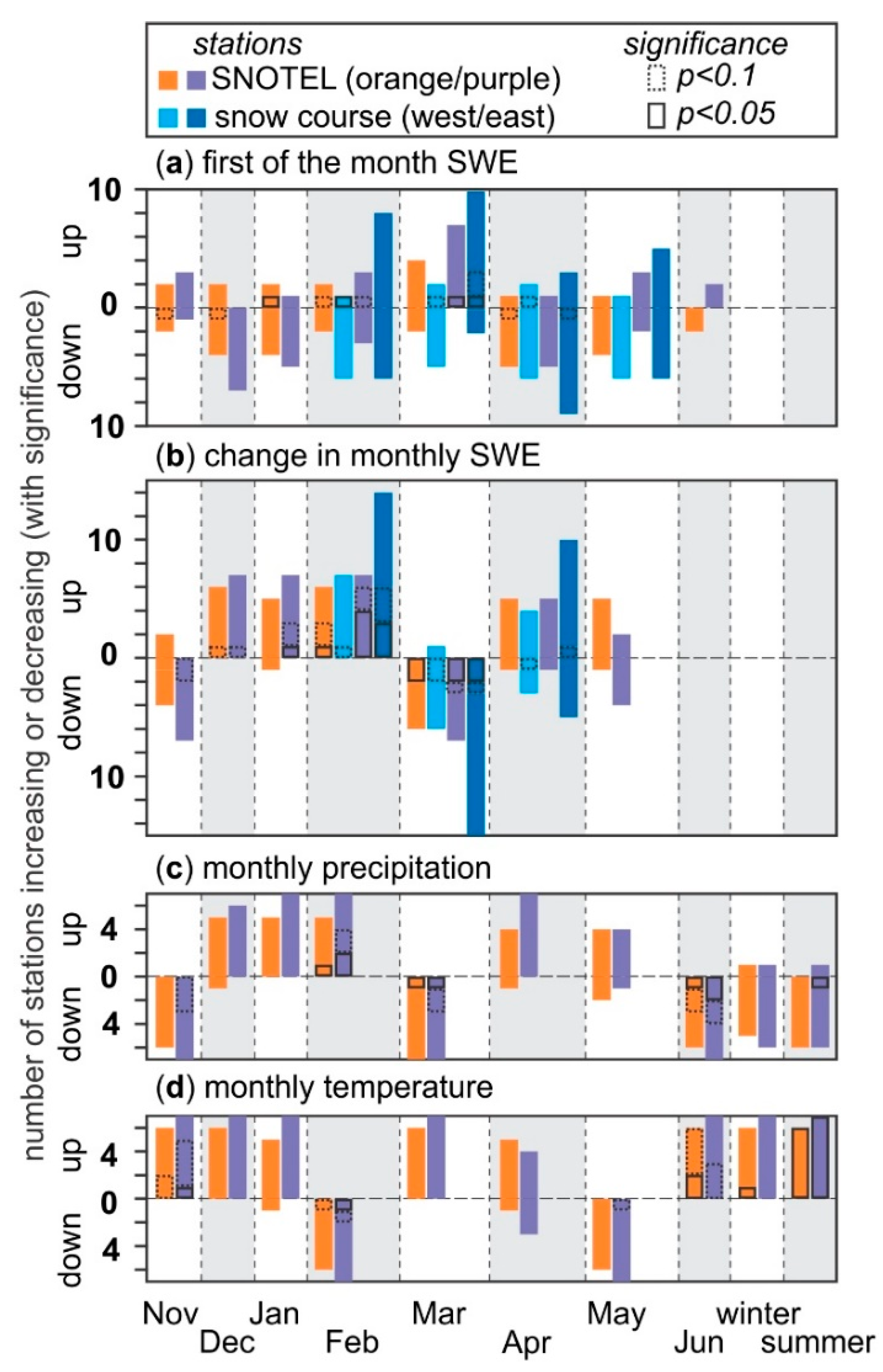
The numbers of stations per month representing the increasing (up) or decreasing (down) trends with the significant (solid line) and marginally significant (dashed line) stations at p < 0.05 and p < 0.10, respectively, characterized by west (orange: Snowpack Telemetry (SNOTEL); light blue: snow course) and east (purple: SNOTEL; dark blue: snow course) stations for (a) first of the month’s snow water equivalent (SWE) trend (see Figure 2); (b) change in monthly SWE trend, (c) monthly precipitation (see Figure 6b), and (d) monthly temperature (see Figure 6c). For (a,b), the snow course stations are included.
Figure 3.
The numbers of stations per month representing the increasing (up) or decreasing (down) trends with the significant (solid line) and marginally significant (dashed line) stations at p < 0.05 and p < 0.10, respectively, characterized by west (orange: Snowpack Telemetry (SNOTEL); light blue: snow course) and east (purple: SNOTEL; dark blue: snow course) stations for (a) first of the month’s snow water equivalent (SWE) trend (see Figure 2); (b) change in monthly SWE trend, (c) monthly precipitation (see Figure 6b), and (d) monthly temperature (see Figure 6c). For (a,b), the snow course stations are included.

Figure 4.
Spatial trends in first-of-month snow water equivalent (SWE) at snow courses and Snow Telemetry (SNOTEL) stations for the period from 1981 to 2015.
Figure 4.
Spatial trends in first-of-month snow water equivalent (SWE) at snow courses and Snow Telemetry (SNOTEL) stations for the period from 1981 to 2015.

Figure 5.
Correlation of monthly (a) snow water equivalent (SWE) trend, and (b) change in SWE with station elevation. Only significant correlations at the p < 0.05 confidence level are shown (solid line); no correlations are significant at the p < 0.10 confidence level. The statistics of these lines are summarized in Table 1a,b.

Figure 6.
Distribution of monthly trends for each month of the snow season (November through May) for all Snowpack Telemetry (SNOTEL) stations (Clow [15]; orange and purple groups) for the period from 1981 to 2015, for (a) change in snow water equivalent (SWE) (includes snow courses, as per Figure 4); (b) precipitation; (c) temperature; and (d) elevation of freeze level or zero-degree isotherm (data from [56]). The freeze-level data were from 2.5° modeled pixels centered at 40° N latitude, with 107.5° W representing the west side of the study area and 105° W representing the east side. For the latter three figures, the season trends for winter from November through May and for summer from June through September are presented. The temperature trends for three non-SNOTEL weather stations are also presented in (c).

Figure 7.
Correlation of monthly (and seasonal for winter, November through May, and summer, June through September) precipitation trend vs temperature trend from Snowpack Telemetry (SNOTEL) stations, divided by (a) west stations (Clow; orange group); and (b) east stations (Clow; purple group); The correlation of (c) first of the next month’s snow water equivalent (SWE) trend and (d) change in monthly SWE trend are presented as bubble size, divided into increasing (blue) and decreasing (red) for all stations on the plots of precipitation trend vs temperature trend.


Table 1.
Correlation statistics of the linear best fit between trends and elevation for (a) first of the month snow water equivalent (SWE) trend (see Figure 4a); (b) change in monthly SWE trend (see Figure 4b); (c) monthly precipitation; and (d) monthly temperature.
| Nov | Dec | Jan | Feb | Mar | Apr | May | Jun | Winter | Summer | |
|---|---|---|---|---|---|---|---|---|---|---|
| (a) First of the Month’s SWE | ||||||||||
| r2 | NS 1 | 0.52 | 0.66 | 0.31 | 0.27 | 0.32 | 0.16 | NS | N/A | N/A |
| Slope | NS | −19.1 | −35.8 | −34.3 | −34.9 | −41.9 | −28.9 | NS | N/A | N/A |
| y-Intercept | NS | 2676 | 2888 | 2926 | 3093 | 2667 | 2812 | NS | N/A | N/A |
| (b) Change in Monthly SWE | ||||||||||
| r2 | 0.47 | 0.56 | NS | NS | NS | NS | NS | N/A | N/A | N/A |
| Slope | −30.4 | −20.8 | NS | NS | NS | NS | NS | N/A | N/A | N/A |
| y-Intercept | 2649 | 3521 | NS | NS | NS | NS | NS | N/A | N/A | N/A |
| (c) Monthly Precipitation | ||||||||||
| r2 | NS | NS | 0.36 | 0.49 | 0.31 | NS | 0.33 | NS | NS | 0.54 |
| Slope | NS | NS | 9.62 | 9.53 | −8.01 | NS | −9.79 | NS | NS | −7.52 |
| y-Intercept | NS | NS | 2793 | 2623 | 2687 | NS | 3025 | NS | NS | 2823 |
| (d) Monthly Temperature | ||||||||||
| r2 | NS | 0.70 | NS | 0.39 | NS | NS | NS | NS | NS | NS |
| Slope | NS | −0.44 | NS | −0.27 | NS | NS | NS | NS | NS | NS |
| y-Intercept | NS | 3376 | NS | 2158 | NS | NS | NS | NS | NS | NS |
Note: 1 r2 is the correlation coefficient; slope is in millimeters per decade per kilometer of elevation, except temperature in degrees Celsius per decade per kilometer of elevation; y-intercept is in meters; all correlations are significant at the confidence level of p < 0.05, except March’s monthly precipitation (c) that is at the confidence level of p < 0.10 and is italicized; NS: not significant.
© 2018 by the authors. Licensee MDPI, Basel, Switzerland. This article is an open access article distributed under the terms and conditions of the Creative Commons Attribution (CC BY) license (http://creativecommons.org/licenses/by/4.0/).
Share and Cite
MDPI and ACS Style
Fassnacht, S.R.; Venable, N.B.H.; McGrath, D.; Patterson, G.G. Sub-Seasonal Snowpack Trends in the Rocky Mountain National Park Area, Colorado, USA. Water 2018, 10, 562. https://doi.org/10.3390/w10050562
AMA Style
Fassnacht SR, Venable NBH, McGrath D, Patterson GG. Sub-Seasonal Snowpack Trends in the Rocky Mountain National Park Area, Colorado, USA. Water. 2018; 10(5):562. https://doi.org/10.3390/w10050562
Chicago/Turabian StyleFassnacht, Steven R., Niah B.H. Venable, Daniel McGrath, and Glenn G. Patterson. 2018. "Sub-Seasonal Snowpack Trends in the Rocky Mountain National Park Area, Colorado, USA" Water 10, no. 5: 562. https://doi.org/10.3390/w10050562
Note that from the first issue of 2016, this journal uses article numbers instead of page numbers. See further details here.