An Unstructured-Grid Based Morphodynamic Model for Sandbar Simulation in the Modaomen Estuary, China


Department of Water Resources and Environment, Pearl River Hydraulic Research Institute, Guangzhou 510611, China
*
Author to whom correspondence should be addressed.
Water 2018, 10(5), 611; https://doi.org/10.3390/w10050611
Submission received: 23 March 2018
/
Revised: 29 April 2018
/
Accepted: 4 May 2018
/
Published: 8 May 2018
(This article belongs to the Special Issue Water Resources and Environmental Fluid Mechanics: From the Glacier to the Lake/Ocean)
Abstract
:The Modaomen Estuary is the most important passageway in discharging flood and sediment of the Pearl River Delta, which is one of the most complex estuarine systems in China. Due to the coupling effect among tidal currents, waves, and sediments, an immense sandbar area evolved in the outer subaqueous delta, impeding the flood releasing during wet season, as well as salinity intrusion during the dry season. In this work, an unstructured-grid based morphodynamic model was proposed to simulate the sandbar evolution process in the Modaomen Estuary. The proposed model was constructed by using the two-dimensional shallow water equations for tidal flow, the advection-diffusion equations for salinity and suspended sediment transport, and the non-equilibrium formulation of the Exner equation for bed evolution. To simulate the wave-induced longshore currents in the Modaomen Estuary, an adaptive time-stepping approach was proposed to couple the unstructured-grid based Simulating WAves Nearshore (SWAN) model and the shallow flow model. An integrated solver is proposed for computing flow, salinity, and sediment transport fluxes simultaneously, and then the shallow water equations and advection-diffusion equations are jointly solved by a high-resolution, unstructured-grid Godunov method. Application of the model to the Modaomen Estuary, using calibrated parameter values, gives results comparable to the measured data. The butterfly shape of the sandbar in the Modaomen Estuary is considerably well simulated by the proposed model, which matches well with the measured topography.
1. Introduction
Sandbars are omnipresent patterns along river estuaries that interact with waves. Their local morphology is expressed in terms of an underwater barrier [1]. An estuary sandbar, which provides natural protection for coastal beaches by reducing inshore wave energy through depth-induced wave breaking [2], is one of the most important morphological units for deltas and estuaries. It can considerably reduce the potential extreme wave run-up during major storms, which would induce severe flood disaster in tidal zones [3]. Moreover, estuary sandbar would play important role in flood releasing during the wet season, as well as salinity intrusion during the dry season.
Sandbar behaves in significantly different ways on different timescales. On shorter timescales of a storm period, rapid offshore sandbar migration might occur due to intense wave breaking over the barrier crest [4]. On longer timescales of several years, sandbars might exhibit a cyclic progressive net offshore migration [5]. To simulate sandbar behavior on different timescales, various kinds of numerical model have been proposed in recent years [2]. Plant et al. [6] proposed a nearshore sandbar migration model based on the break point paradigm using the wave-height dependent equilibrium location. Pape et al. [7] presented a data-driven model of sandbar migration by adopting neural networks. The recent process-based models, which mostly use the wave phase-averaged method, have succeeded in simulating the dynamic evolution of the surfzone sandbar profile on timescales of days and weeks to years with reasonable accuracy [8,9,10,11]. Those process-based, one-dimensional cross-shore models [2,8] could take into account the coupling effect among tidal currents, waves and sediments, which has been shown to be an important dynamic factor that drives estuary sediment transport. However, those process-based models still have some limitations. For example, the one-dimensional cross-shore models can not accurately simulate the plane shape of the sandbar, which is very important for coastal engineering design and estuary management. Moreover, the respective contributions of different dynamic factors to sandbar evolution are still not fully understood [2], so the modeling details on the key processes governing sandbar behavior need to be improved.
The Pearl River Delta is one of the most complex estuarine systems in China. Freshwater and sediments of the Pearl River basin are discharged by eight “gates” into the estuarine bays, and the Modaomen Estuary is the biggest gate with regard to the water delivery and sediment discharge. Due to the coupled effect of tidal currents, waves, and sediments, an immense sandbar area evolved in the Modaomen Estuary. The estuary sediment dynamics, which involve several processes such as advection, diffusion, erosion, aggregation, settling, deposition, and consolidation of the deposits [12], play an important role in the formation and evolution of estuary sandbar with complex depositional patterns. The flow and sediment movement in the Pearl River estuary are not only affected by the runoff and sediment inputs from the upstream catchments, but also significantly regulated by the tidal currents and sediment movement in the South China Sea. Besides, the sediment movement is affected by many factors including waves, wind, salinity, and so on. Although waves have a minor effect on the current under strong runoff in the wet season, with a change in current of no more than 0.07 m/s [13], the “wave lifting sand” effect should be considered by the numerical models. Besides, currents exert a significant effect on waves. The ebbing flow increases wave height and the flooding flow decreases wave height within a tidal period [13]. Wave height varies consistently with the tide level inside the mouth bar, while wave height has a phase lag of about one-quarter of the tidal period outside the mouth bar [13]. Those complex coupling effects among tidal currents, waves, salinity and sediments should be fully considered by models. On the other hand, if the interactions between tidal currents and waves are not considered, the sediment transport of coastal currents, which is produced by the wave radiation stresses, is ignored by numerical models. Besides, as the flocculation effects of salinity and the “wave lifting sand” effects are very important for sediment transport, numerical models would predict incorrect results if the interactions among tidal currents, waves, salinity and sediments were not considered.
As a result of sediment re-suspension induced by waves, as well as sediment transport by tidal currents, the sediment movement in the Pearl River estuary is very complicated. So morphodynamic approaches based on the coupled wave-current-sediment transport model [14] should be adopted for sandbar simulation in the Modaomen Estuary. To numerically reproduce the sediment transport process, Zhu et al. [15] established a 3D unstructured triangular gird cohesive sediment model for the Pearl River Estuary. Yin et al. [16] proposed a coupled model that combines the typhoon model, hydrodynamic model (Delft3D-FLOW), wave model (Delft3D-WAVE) and sediment transport model (Delft3D-SED) for the region of the Pearl River Estuary. Model verifications showed that the coupled model performed well in reflecting the characteristics of the typhoon field, tidal currents, wave height, storm surge, and distribution of suspended sediment in the studied region. Chen et al. [17] proposed a 3D transport model of suspended solids in the Pearl River estuary. The modeled results showed that the suspended solids inflowing from the eight rivers transport southwestwards with the carry of strong coastal flow in the Pearl River estuary. Although several numerical models have been proposed to simulate the sediment transport as well as bed evolution in the Pearl River estuary, sandbars in the Modaomen Estuary are still not well simulated. The key issue that needs to be resolved is that the coupling effect among tidal currents, waves, salinity, and sediments should be properly treated by the numerical model. Moreover, there are few studies on adopting the robust and well-balanced finite volume model [18], which is based on the improved formulation of shallow water equations and sloping bottom model together with VFRs (volume/free-surface relationships) [18], as the basic hydrodynamic model for sediment transport simulation.
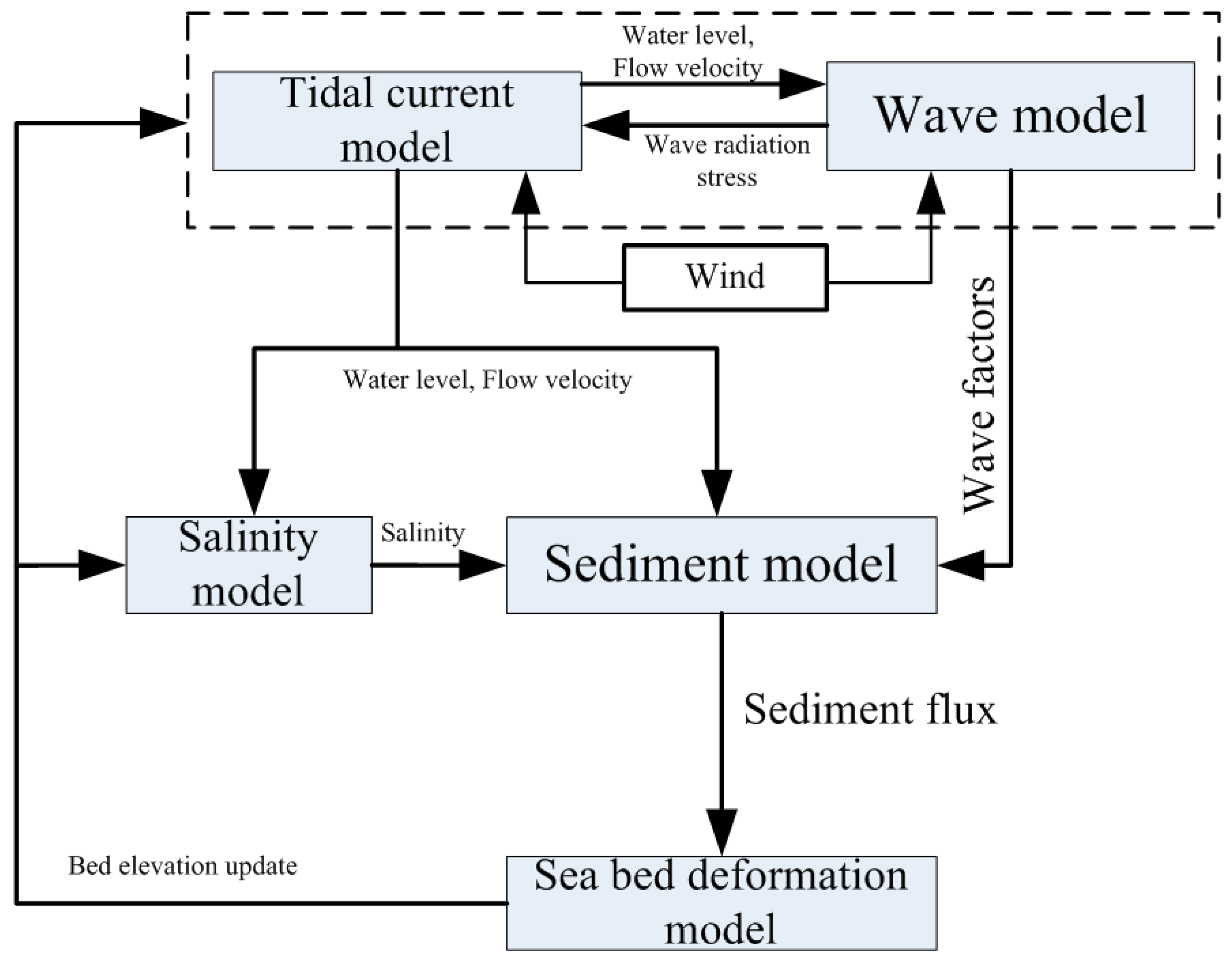
In this work, the robust and well-balanced shallow water model is adopted to couple with a wave model, and an unstructured-grid based, two-dimensional morphodynamic model is developed for sandbar simulation in the Modaomen Estuary. In order to simulate the process of “wave-lifting-sand, tidal-current-transporting-sand” in the Lingding Sea, a conceptual framework for coupling the tidal currents, waves, salinity, and sediment models is proposed to develop the coupled model, in which the tidal current model, wave model, salinity model, and the sediment model are tightly coupled with each other. To simulate the wave-induced longshore currents, an adaptive time-stepping approach is proposed to couple the unstructured-grid based Simulating WAves Nearshore (SWAN) model and the shallow flow model. The effect of waves on sediment transport is considered by using the sediment-carrying capacity and the condition of sediment incipient motion.
This paper is organized as follows: Section 2 presents the governing equations for the circulation model, suspended load, salinity, and waves. Section 3 presents the sediment transport module, in which the treatments of the key issues in sediment calculation are discussed. Section 4 presents the numerical methods and the coupling approach. In Section 5, the proposed numerical model is validated against a case study of sandbar simulation in the Modaomen Estuary, China. Brief conclusions are given in Section 6.
2. Governing Equations
2.1. Governing Equations for the Circulation Model
The improved two-dimensional shallow water equations [18] in conservation formulation, further integrating the wave radiation stresses, are adopted as governing equations for the circulation model:
in which, U denotes the vector of conservation variables; Eadv, Gadv denote the vector of convective flux in the x- and y-coordinates, respectively; Ediff, Gdiff denote the vector of diffusion flux in the x- and y-coordinates, respectively; and S represents the source terms:
in which, h is the water depth; u, v are velocities in the x-, and y-coordinates, respectively; b is the bed elevation; νt is the turbulent viscosity coefficient, and , , is the von Karman’s constant, where is the shear velocity; g is the gravitational acceleration; f is the Coriolis force coefficient; denotes the wind stress, and , , is the wind drag coefficient, where and are the wind speeds measured at 10.0 m above the sea level in the - and -directions, respectively, is the density of water, and is the density of air; Sxx, Sxy, Syx, Syy are wave radiation stresses; and are friction slopes in the - and -directions, respectively; and and are bed slopes in the - and -directions, respectively. The friction slopes are estimated by using the Manning formulae:
in which, n is the empirical Manning coefficient.
2.2. Governing Equations for Suspended Load
The following advection-diffusion equation is used as the governing equation for suspended load,
in which, the superscript k denotes the k-th groups of sediment diameters; S denotes the sediment concentration; νsx, νsy denote the turbulent diffusion coefficients, which are calibrated constant parameters for simplification; and Fs denotes the scour and deposit rate.
The sediment-carrying capacity is used to represent the function of scour and deposit, as well as the equation of bed deformation, which is given by [19],
in which, α1, α2 denote the saturation recovery coefficients of sediment concentration and sediment-carrying capacity, respectively; α3 denotes the settling probability; ω denotes the sediment settling velocity; S* denotes the sediment-carrying capacity; ρs denotes the sediment density; and α1, α2 and α3 are calibrated constant parameters.
2.3. Governing Equations for Salinity
The following advection-diffusion equation is used as the governing equation for salinity,
in which, c is the salinity, which is measured and expressed by the chlorinity; and Dx, Dy are diffusion coefficients of the salinity, which are calibrated constant parameters for simplification.
It should be noted that, in the proposed coupled model, salinity plays a role only in the evaluation of the sediment settling velocity. Since the settling velocity is an important factor for sediment transport, salinity must be considered by numerical models.
2.4. Governing Equations for Waves
The spectral action balance equation is used as the governing equation for waves, which is given by [20],
in which, N is the action density; σ is the relative radian frequency; θ is the wave propagation direction; Cx, Cy are the propagation velocities of wave energy in spatial x-, y-space, respectively; Cσ, Cθ are the propagation velocities in spectral σ-, θ-space, respectively; and S(σ, θ) is the source/sink term that represents all physical processes which generate, dissipate, or redistribute wave energy. The source/sink term represents the wave growth by the wind, nonlinear transfer of wave energy through three-wave and four-wave interactions and wave decay due to whitecapping, bottom friction and depth-induced wave breaking.
Using the linear wave theory and the conversion of wave crests, the wave propagation velocities in spatial space within the Cartesian framework and spectral space can be obtained from the kinematics of a wave train [20]:
in which, s is the space co-ordinate in the wave propagation direction of θ, and m is a co-ordinate perpendicular to s; is the wave speed; and is the tidal current velocity.
3. Sediment Transport Module
In the Pearl River estuaries, the characteristic sediment diameters are 0.002, 0.005, 0.01, 0.025, 0.05, 0.1, 0.25, 0.5, 1.0, and 5.0 mm. The correspondingly accumulative grading compositions are 32.0%, 56.5%, 76.5%, 85.8%, 92.7%, 97.1%, 99.6%, 100.0%, 100.0%, and 100.0%. Therefore, it can be concluded that the diameter of most sediment is smaller than 0.063 mm, and the deposit of sediment at the estuaries is mostly constituted by mud. So in this work, we neglect sand material completely and adopt formulations that deal with cohesive material only.
3.1. The Calculation of the Settling Velocity of Sediment
The Zhang Ruijin formula [21] is adopted for computing the settling velocity of sediment, which is given as,
in which, ν denotes the kinematic viscosity coefficient (1.01 × 10⁻⁶ m2/s); d denotes the sediment grain size; γ denotes the specific gravity of water; and γs denotes the specific gravity of sediment.
With the increase of cohesive sediment concentration, the group settling velocity increases due to the flocculation. Therefore the Richardson & Zaki formula [22] is used to correct the settling velocity,
in which, the superscript k denotes the k-th groups of sediment diameters; Ns is the number of groups; denotes the corrected settling velocity; denotes the settling velocity computed by Equation (11), using the corrected kinematic viscosity coefficient νm for muddy water; Cμ is the correction coefficient of sediment concentration; Sv is the concentration of muddy water in the form of the volume ratio, and Sv = S/ρs; Svm is the limit concentration of muddy water in the form of the volume ratio; and dk, Pk are the representative diameter and weight percentage of the k-th grain-size fractions, respectively.
Furthermore, the salinity and sediment grain size have a direct impact on sediment flocculation and settling. Considering the flocculation effect of salinity, the settling velocity of sediment is corrected by the following equations [23], which are obtained from measured data in the Pearl River Estuary.
Study shows that there is the following relationship between the flocculation settling velocity, the sediment practical size and the deposition distance [23]:
in which, denotes the settling velocity with flocculation; and R denotes the deposition distance.
Based on Equation (16), if the chlorinity is lower than or equal to 20 psu, then [23]
Otherwise, i.e., the chlorinity is higher than 20 psu, then [23]
in which, is the corrected settling velocity by considering salinity, which is used in Equation (4) of the function of scour and deposit.
3.2. The Initiation Condition of Sediment Movement
The Zhang Ruijin formula [21] is adopted for computing the incipient velocity,
in which, the superscript k denotes the k-th groups of sediment diameters; and Uc denotes the incipient velocity.
The formula of wave height for the initiation of sediment movement developed by Dou Guoren [24] is adopted in this work,
in which, T denotes the wave period; L denotes the wave length; Δ denotes the bed roughness height; δ = 2.3 × 10⁻⁵; ε0 denotes the bonding strength; β denotes the infilled aggregate coefficient in sediment; βw denotes the infilled aggregate coefficient in waves; and a, b denote the constant coefficients, which are determined by experimental data of sediment incipient motion under the wave.
Based on Equations (19) and (20), the initiation condition of sediment movement is given by,
and,
in which, U is the velocity of tidal current and H is the significant wave height.
So Equation (4) is equivalent to the following equations,
3.3. The Sediment-Carrying Capacity
Based on the analysis of the measured data in the Pearl River Delta, the sediment-carrying capacity of the tidal flow is proportional to the third power of the tidal flow velocity, and is inversely proportional to the settling velocity and water depth. In this work, the sediment-carrying capacity of the water flow proposed by Zhang Ruijin [21] is adopted, which is given as,
in which, denotes the sediment-carrying capacity of the water flow; and k, m denote the empirical parameters.
The sediment-carrying capacity of the waves proposed by Dou Guoren [24] is adopted in this work,
in which, denotes the sediment-carrying capacity of the waves; α0, β0 denote the empirical parameters; and Hs denotes the significant wave height.
The carrying capacity for a wave-current coexistent system is computed by,
in which, is the total sediment-carrying capacity.
3.4. Adjustment of Bed-Load Gradation Composition
The concept of a mixing layer is introduced in this work to construct the relationship between the bed-load gradation composition and the erosion strength, which is given by [25],
in which, Hm denotes the thickness of the mixing layer; Pb,k denotes the thickness ratio of the k-th grain-size fractions; Bm denotes the width of the mixing layer; Gk denotes the flux of sediment transport, which is the sum of the convection flux and diffusion flux of Equation (3); ε denotes the porosity of the bed material; and Pb0,k denotes the thickness ratio of the bed material below the lower boundary of the mixing layer.
To adjust the bed-load gradation composition, the sea bed is divided into four layers. The top layer is the layer for sediment exchange between the bed material and the suspended sediment. The two middle layers are designed for the transition from the top layer to the bottom layer. Both the settlement of suspended sediment and the re-suspension of bed material will first induce the adjustment of bed-load gradation composition at the top layer. Following this, the thicknesses of the top layer and two middle layers are assumed to remain constant, so the bed-load gradation composition of the two middle layers and the bottom layer, as well as the thickness of the bottom layer, are adjusted by using the conservation law.
Assume that the initial thickness ratio of the bed material of the n-th layer is , and the subscript n denotes the layer index (from top layer to bottom layer, n = 1, 2, 3, 4). If the thicknesses of erosion-sedimentation of the bed and the k-th groups of sediment are and , then the thickness ratio of the bed material of the partial top layer, which is above the bottom surface of the former top layer, is updated by,
in which, is the updated thickness ratio of the bed material; H1 is the thickness of the top layer.
So for the case of sedimentation (), the bed-load gradation composition is adjusted by,
For the case of erosion (), the bed-load gradation composition is adjusted by,
in which, is the updated thickness ratio of the bed material of the n-th layer; H2 and H3 are the thicknesses of the middle layers, and it should be noted that H1, H2, and H3 are assumed to remain constant; and and are the initial and updated thickness of the bottom layer, respectively.
4. Numerical Methods
4.1. Numerical Method for Tidal Currents Model
The robust well-balanced finite volume method proposed by Song et al. [18,26,27] is adopted in this work for numerical resolving the governing equations of tidal currents. The method uses a high-resolution finite volume Godunov-type scheme with the HLLC (Harten, Lax, vanLeer, Contact) approximate Riemann solver [18]. The MUSCL (Monotone Upstream Scheme for Conservation Law) reconstruction technique is used to achieve second-order accuracy in space, and the second-order accuracy in time is obtained by using Hancock’s predictor-corrector scheme [27]. Details about the numerical method can be found in the references [18,26,27]. Briefly, the process of time stepping is as follows:
Step 1: Calculate the limited gradient by central values for each cell.
Step 2: Calculate the predictor results for each cell. The predictor results are given by,
in which, is the water level; is the computational time step controlled by the CFL (Courant-Friedrichs-Lewy) condition; and denote the limited gradient in the - and -directions respectively; and the superscripts and denote the current time step and the predictor step, respectively.
Step 3: Calculate the reconstructed values for each edge.
Step 4: Calculate the numerical fluxes for each edge. The HLLC approximate Riemann solver is adopted to compute face fluxes, which is given by
where and denote the reconstructed values; and are wave speeds. More details about the HLLC solver can be found in Song et al. [18].
Step 5: Calculate the source terms approximation for each cell.
Step 6: Calculate the solutions at the next time step for each cell. The solutions at the next time step k + 1 are given as,
where and are the edge number and length respectively; is the numerical flux; is the area; and is the source approximation. The superscripts denote that the reconstructed variables are computed on the predictor results.
4.2. Numerical Method for the Coupled Tidal Current and Wave Models
To simulate the offshore wave propagation and coastal currents in the Pearl River Delta region, the two-dimensional tidal current model and the third generation wave model SWAN are adopted to develop a coupled hydrodynamic model. The dynamic coupling between the tidal current model and wave model is constructed by considering the wave radiation stress in the tidal current model, as well as the influence of tidal flow on waves in the wave model. The tidal current model and wave model are executed alternately. As the wave model uses a bigger fixed time step, while the time step of tidal current model is dynamically limited by the CFL condition, an asynchronous approach is adopted for the coupling of the tidal current model and wave model. So an adaptive time-stepping method is used for the tidal current model to trace the time line of the wave model, which is given as,
in which, ∆tswan is the fixed computational time step of wave model; ∆tFlow is the adaptive computational time step of the tidal current model; the superscript M is the amount of run steps required for the tidal current model to trace the time line of the wave model; and the superscript i is the index of run step for the tidal current model.
Equation (38) means that, the adaptive computational time step of tidal current model is limited by the CFL condition for i = 1, 2, M − 1, while it is limited by Equation (38) for i = M. The amount of run steps required for the tidal current model to trace the time line of the wave model, M, satisfies the following relationship,
in which, denotes the CFL-limited computational time step of tidal current model at the M-th run step.
4.3. Numerical Method for the Advection-Diffusion Equation
Assume that the water flow fluxes are denoted as FWF = (F1, F2, F3), in which F1 denotes the flux of water volume, and F2 and F3 denote the momentum fluxes. The integrated solver proposed by Song et al. [28,29] is adopted for computing flow and mass transport fluxes simultaneously, which is given by,
in which, Fadv denotes the convection flux; and cL, cR denote the reconstructed concentration values from the left-cell and the right-cell, respectively.
In Equation (40), F1 > 0 means that water flows from the left-cell to the right-cell, and F1 < 0 means that water flows from the right-cell to the left-cell.
By using the divergence theorem, the diffusion flux of mass transport is given by,
in which, Fdif is the diffusion flux; , are the reconstructed water depth from the left-cell and the right-cell, respectively; and nx, ny are the components of the unit outward normal vector.
Similar to the tidal current model, the MUSCL reconstruction technique is used to achieve second-order accuracy in space, and the second-order accuracy in time is obtained by using Hancock’s predictor-corrector scheme. Details about the numerical method for resolving the advection-diffusion equation can be found in the references [28,29]. Briefly, the process of time stepping is as follows:
Step 1: Calculate the limited gradient by central values for each cell.
Step 2: Calculate the predictor results for each cell. The predictor results are given by,
in which, is the computational time step of tidal current model; and denote the limited gradient in the - and -directions respectively; and the superscripts and denote the current time step and the predictor step, respectively.
Step 3: Calculate the reconstructed values for each edge.
Step 4: Calculate the numerical fluxes for each edge.
Step 5: Calculate the source terms approximation for each cell.
Step 6: Calculate the solutions at the next time step for each cell. The solutions at the next time step k + 1 are given as,
where m and L are the edge number and length respectively; F is the numerical flux; is the area; and S is the source approximation.
It should be noted that, the numerical method described above can be applied in the same way to solve Equation (3) of suspended load, as well as to solve Equation (5) of salinity.
4.4. The Coupling Approach
5. Case Study: Sandbar Simulation in the Modaomen Estuary, China
5.1. The Study Area
To simulate the sandbar in Modaomen Estuary, the Lingding Sea is selected for this case study (see in Figure 2). The width of the study area is about 112 km, the length is 125 km, and the total waters area is about 7000 km2.
5.2. Computational Grids and Topography
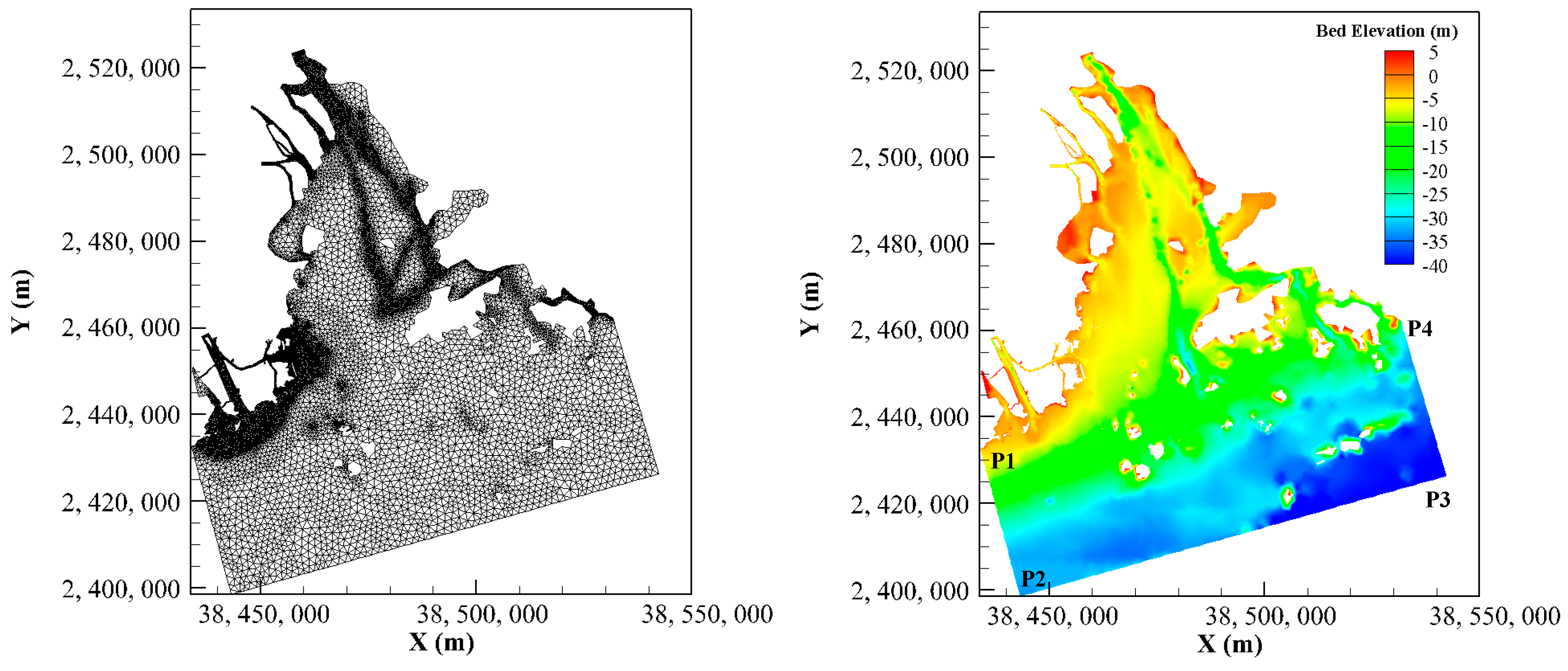
Figure 3 shows the computational grids, and the bed elevation. The upstream boundaries include Dahu station, Nansha station, Fengmamiao station, Hengmen station, and Denglongshan station (see in Figure 2). The western boundary reaches to Zhuhai airport, and the eastern boundary reaches to Hong Kong waters (see in Figure 2). P1-P2-P3-P4 are the tidal level boundaries (see in Figure 3). The number of computational grids is 51,800, of which the minimum edge length is 5 m, and the minimum grid area is 20 m2.
5.3. Model Parameters
- (1)
- Parameters of the tidal currents model. The CFL (Courant-Friedrichs-Lewy) number is set to 0.85. The empirical Manning coefficient varies from 0.012 to 0.025, and it generally varies inversely as the water depth.
- (2)
- Parameters of the salinity model. The computational time step for the salinity model is equivalent to that of the tidal currents model. The diffusion coefficients of the salinity vary from 50 to 150 m2/s. It should be noted that the diffusion coefficients are calibrated by simulating other events in the Lingding Sea.
- (3)
- Parameters of the wave model. The threshold depth, i.e., in the computation any positive depth smaller than the threshold depth is made equal to the threshold depth, is set to 0.05 m. The maximum value for the wind drag coefficient is set to 0.0025. The maximum Froude number is set to 0.8. The lowest discrete frequency that is used in the calculation is set to 0.055, and the number of meshes in theta-space is set to 36. The SWAN code run in third-generation mode for wind input, quadruplet interactions and whitecapping.
- (4)
- Parameters of the sediment model. The number of characteristic sediment diameter is 10, and the characteristic sediment diameters are 0.002, 0.005, 0.01, 0.025, 0.05, 0.1, 0.25, 0.5, 1.0, and 5.0 mm. The correspondingly initial accumulative grading compositions, for example, are 32.0%, 56.5%, 76.5%, 85.8%, 92.7%, 97.1%, 99.6%, 100.0%, 100.0%, and 100.0%. It should be noted that there are different accumulative grading compositions, and the initial spatial distributions of the accumulative grading compositions for both the suspended load and the sea bed were set through practical experience in the Pearl River Delta. The sea bed is divided into four layers, and from the top layer to the bottom layer, the initial thicknesses of each layer are 0.05, 0.10, 0.5, and 2.0 m, respectively. Those thicknesses were also set through practical experience in the Pearl River Delta. The computational time step for the sediment model is equivalent to that of the tidal currents model. The diffusion coefficients of the suspended load vary from 5 to 20 m2/s. The empirical parameters k, m, which are used to compute the sediment-carrying capacity of the water flow, are set to 0.013, 0.24 when the water depth is smaller than 1.0 m; otherwise, if the water depth is smaller than 3.0 m the k, m are set to 0.08, 0.54, respectively; otherwise, the k, m are set to 0.10, 0.55, respectively. The empirical parameters α0, β0, which are used to compute the sediment-carrying capacity of the waves, are set to 0.023, 0.0004, respectively. To limit the sediment-carrying capacity, a maximum value of 4.5 kg/m3 is used for the water flow, while a maximum value of 0.5 kg/m3 is used for the waves. The settling probability, α3, is set to 1.0, and the saturation recovery coefficients of sediment concentration and sediment-carrying capacity, α1 and α2, are set to 0.05 and 1.0 when S ≥ S*; and are set to 0.5 and 1.0 when S < S*, respectively.
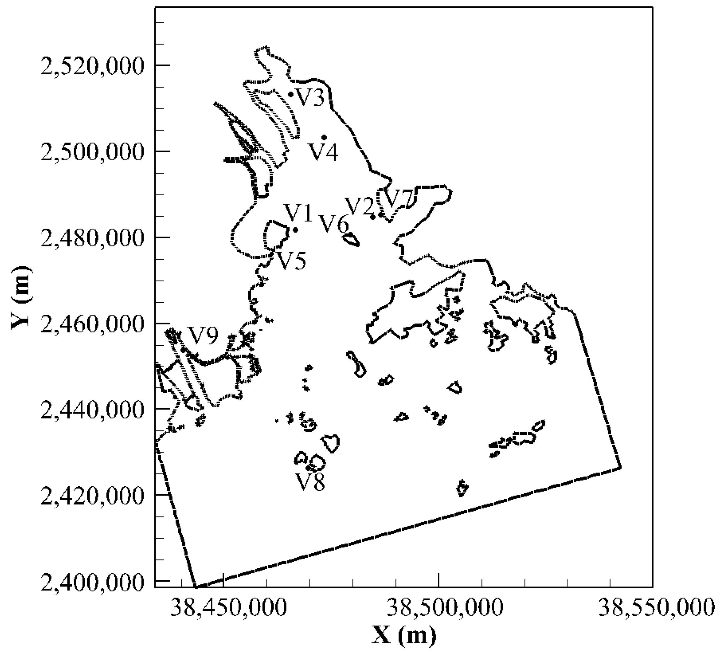
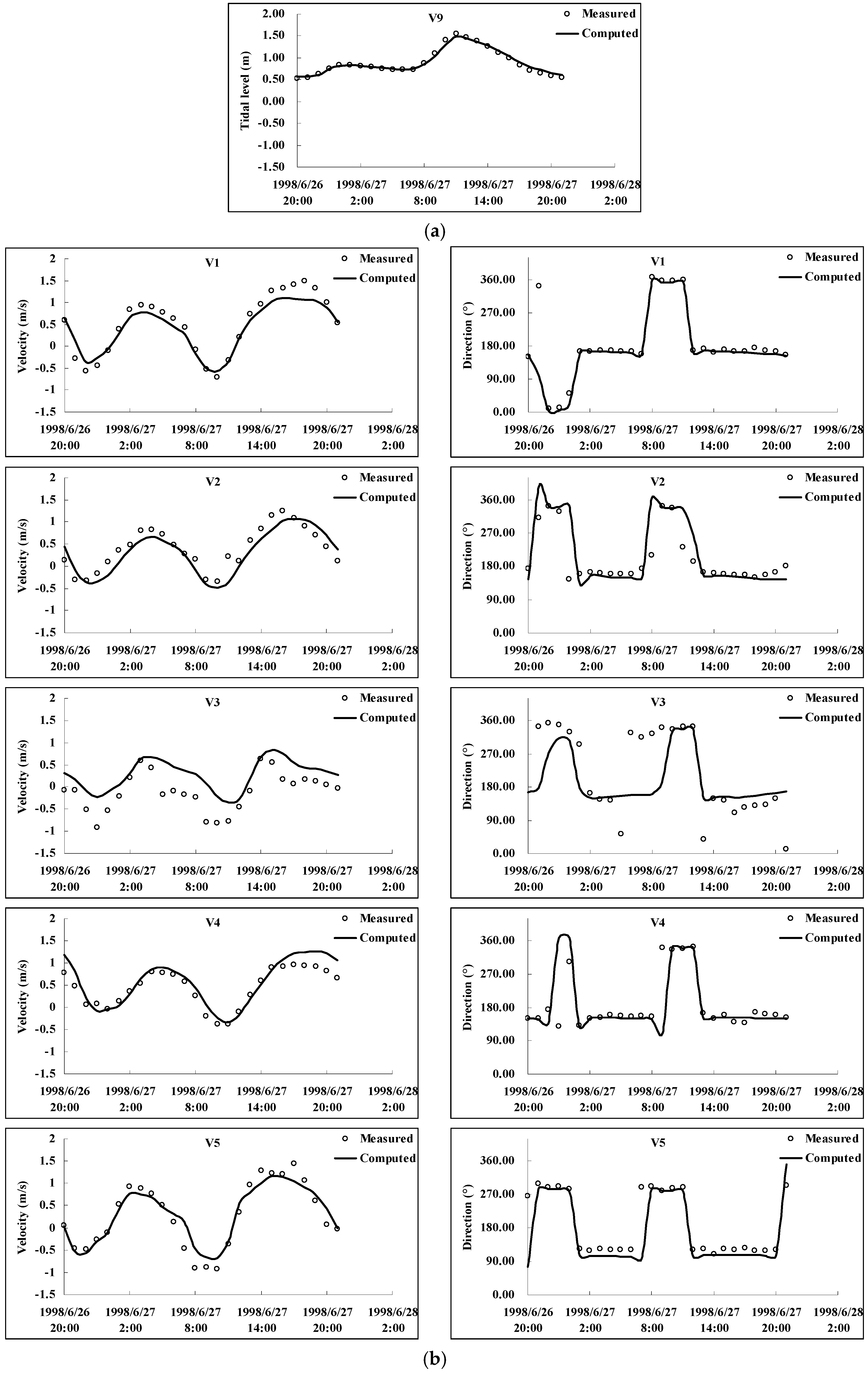
The measured data, including tidal level, velocity, and sediment concentration, from 26 June 1998 20:00 to 27 June 1998 21:00 were used for parameter validation. Figure 4 presents the positions of the measuring points V1–V9.
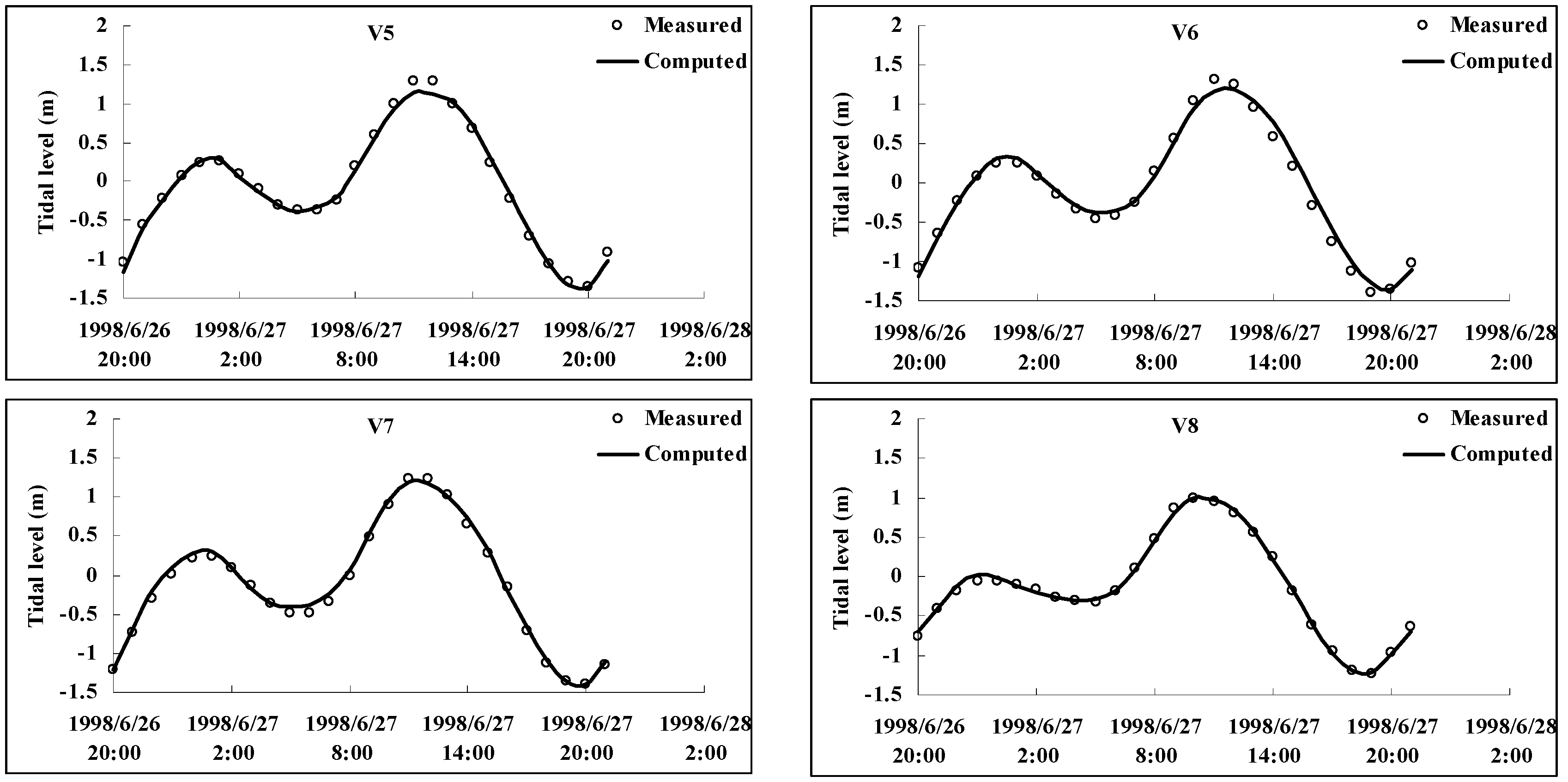
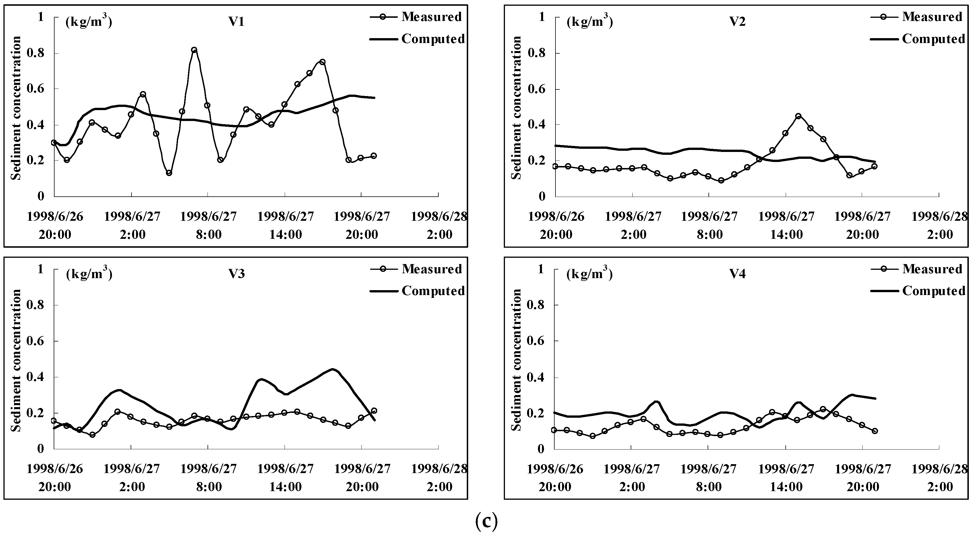
Figure 5a presents the comparison of the tidal levels between the numerical results and the measured data; Figure 5b presents the comparison of the flow velocities and directions between the numerical results and the measured data; Figure 5c presents the comparison of the sediment concentration between the numerical results and the measured data. From Figure 5 it can be seen that the computed tidal levels, flow velocities and directions match well with those from the measured data, and the simulated sediment concentrations are consistent with that of the measured data, validating the reliability of the model parameters.
5.4. Boundary Conditions
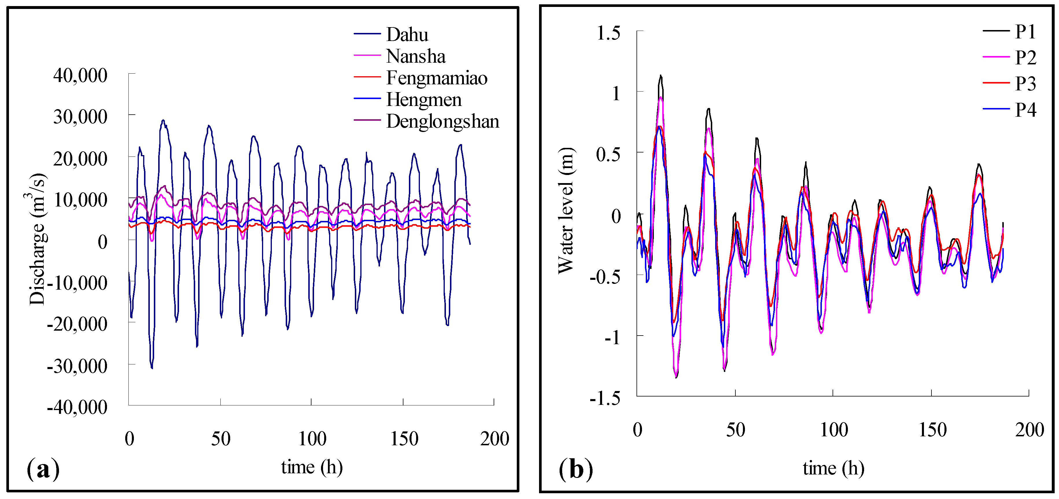
The combined conditions of the “99.7” flood season are used in this work for simulation. The “99.7” flood season denotes a flood that happened in July 1999. The time period was 15 July1999 23:00~23 July 1999 17:00, and the flood during this time was about 200 h. The “99.7” peak discharge of Sanshui station, which is an upstream hydrology control station in the Pearl River Delta, was 9200 m3/s and was close to the mean annual peak discharge of 9640 m3/s. Besides this, the “99.7” peak discharge of Makou station, which is another upstream hydrology control station in the Pearl River Delta, was 26,800 m3/s and was close to the mean annual peak discharge of 27,600 m3/s. Thus, it can be concluded that the combined conditions of the “99.7” flood season could be chosen as a typical dynamic condition for the flood season. Furthermore, the combined conditions of the “2001.2” dry season should be chosen as a typical dynamic condition for the dry season. In this work, we only present the results of the “99.7” flood season for simplification. Figure 6 presents the boundary conditions of the tidal currents model, including discharges at Dahu station, Nansha station, Fengmamiao station, Hengmen station, and Denglongshan station, and tidal levels at P1–P4. From Figure 6, it can be seen that the computational period was about 200 h, and during this period the amount of water delivery of Dahu station, Nansha station, Fengmamiao station, Hengmen station, and Denglongshan station are 368,937, 405,458, 206,921, 289,548, and 558,068 × 104 m3, respectively. It should be noted that the large difference in discharge was due to the tidal current; positive discharge indicates an ebb tide, while negative discharge indicates a flood tide.
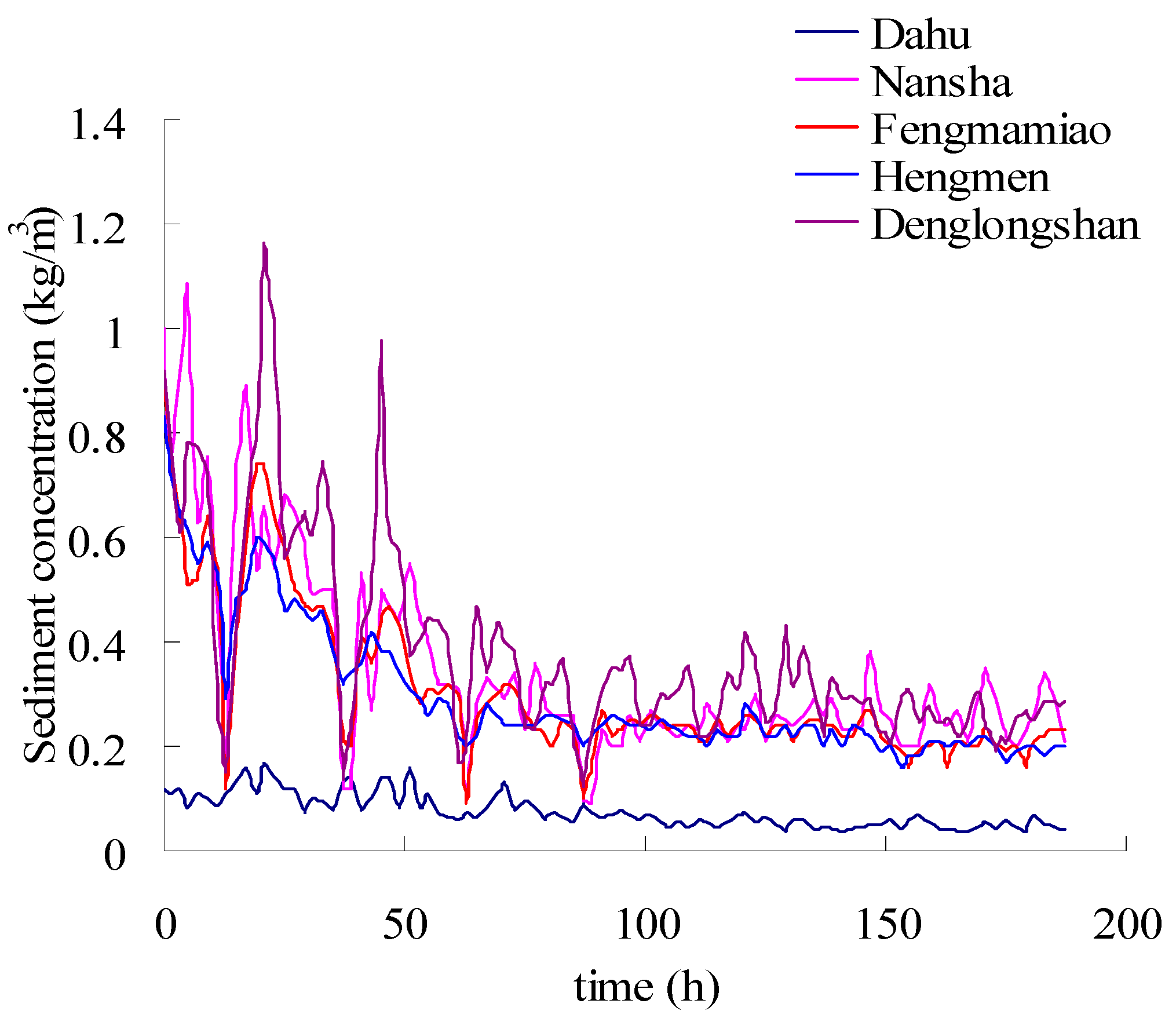
Figure 7 presents the boundary conditions of the sediment model, from which it can be seen that the maximum sediment concentration is 1.2 kg/m3, and the averages are 0.07, 0.34, 0.30, 0.29, and 0.37 kg/m3 for Dahu station, Nansha station, Fengmamiao station, Hengmen station, and Denglongshan station, respectively. A steady wind condition is used in this case, the wind speed is 3.6 m/s, and the wind direction is SE. This corresponds to the statistical value of the Dawanshan Station for the flood season. Since the wind wave is the dominant wave pattern in the Lingding Sea, the steady wind condition is appropriate for the wave and sediment simulation.
5.5. Model Validation and Discussion
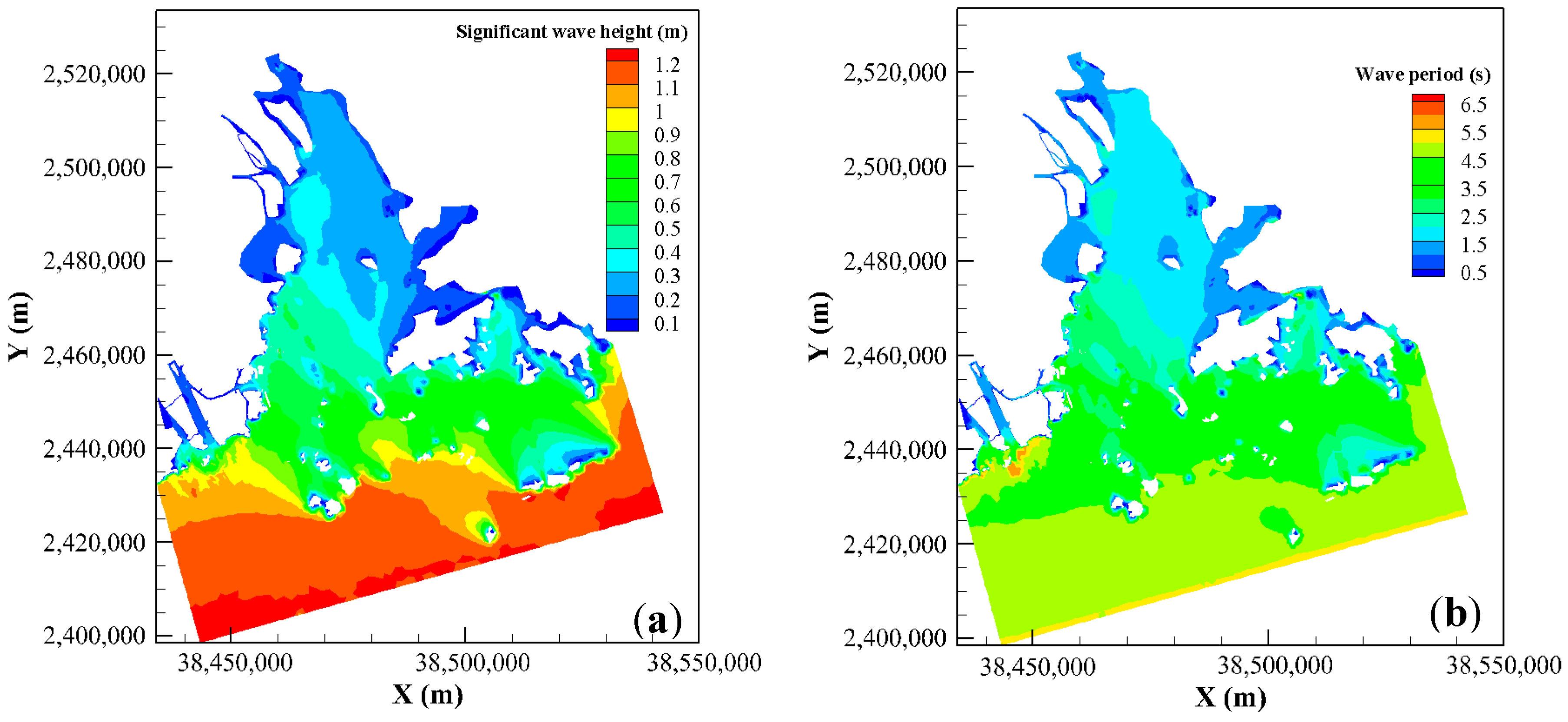
Figure 8 shows the simulated distribution of significant wave height and the wave period. From Figure 8 it can be seen that the significant wave height was about 0.5 m~1.0 m in Modaomen Estuary, while the wave period was about 4.5 s~5.5 s.
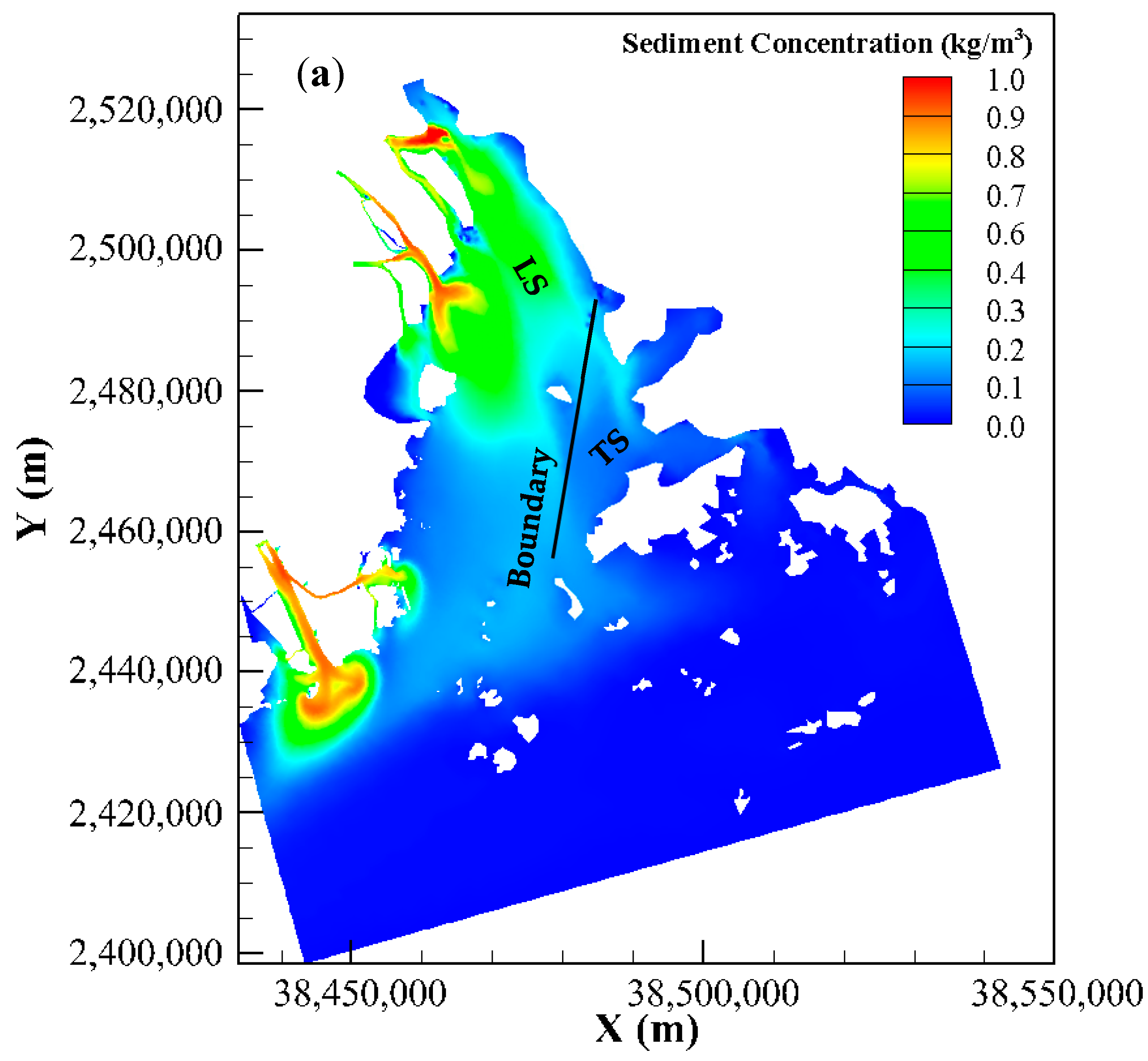
Figure 9 shows the simulated distribution of sediment concentration at flood fast tide and at ebb fast tide. It should be noted that the moments of flood fast tide and ebb fast tide are confirmed with regard to the Modaomen Estuary, and there is a phase difference of tidal current between the Modaomen Estuary and other northern estuaries. From Figure 9 it can be seen that the sediment concentrations near river estuaries are much higher than those of other areas. Especially, near the Modaomen Estuary, the sediment concentration at ebb fast tide is much higher than that at flood fast tide. So it can be concluded that the tide is the dominant factor influencing the variation of suspended sediment concentration. Similar results were found in Deep Bay, Pearl River Estuary, China [30]. Besides, the diffusion phenomenon of suspended load is well reproduced in Figure 9. The high sediment concentration zone along the shoreline indicates the effect of “wave-lifting-sand, tidal-current-transporting-sand” in the Lingding Sea.
From Figure 9 it can be concluded that the northwestern estuaries of the Lingding Sea, including Humen, Hengmen, Jiaomen, Hongqimen, and Modaomen, are the main inputs of the suspended sediment, since freshwater and sediments of the Pearl River basin are discharged by these estuaries into the Lingding Sea, and the Modaomen Estuary is the biggest gate with regard to the water delivery and sediment discharge. During the flood season, the suspended sediment concentration of the Pearl River is much higher than that of “wave-lifting-sand”, so it can be concluded that these estuaries of the Pearl River provide most of the suspended sediment. The sediment concentration near those estuaries is obviously higher than that of other waters. Especially, the boundary (see in Figure 9) from Lingding shallows (LS) to Tonggu shallows (TS), by which the Lingdingyang Sea can be divided into two parts regarding the relatively higher/lower sediment concentration, is considerably well simulated. As a whole, the simulated result of sediment concentration distribution is in accordance with that of the actual situation [31], i.e., in the Lingdingyang Bay, under the influence of the strong tidal flow on the east-side, the sediment is transported southward along the west-side, and spread to the east-side. The sediment concentration distribution is higher on the west-side and lower on the east-side, and higher on the north-side and lower on the south-side [31]. Moreover, the suspended sediment dynamics computed by the proposed model match well with other research results [32,33].
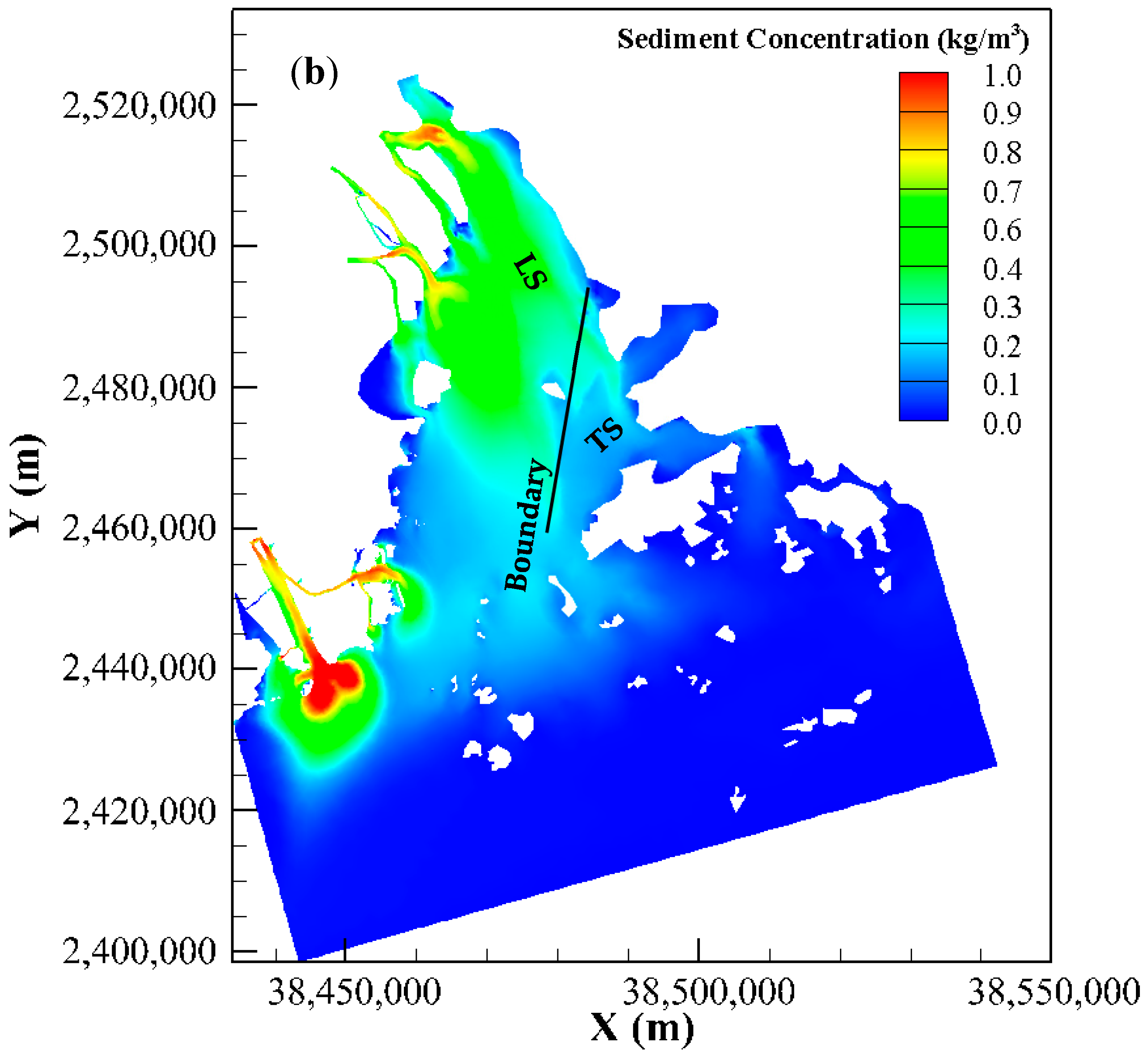
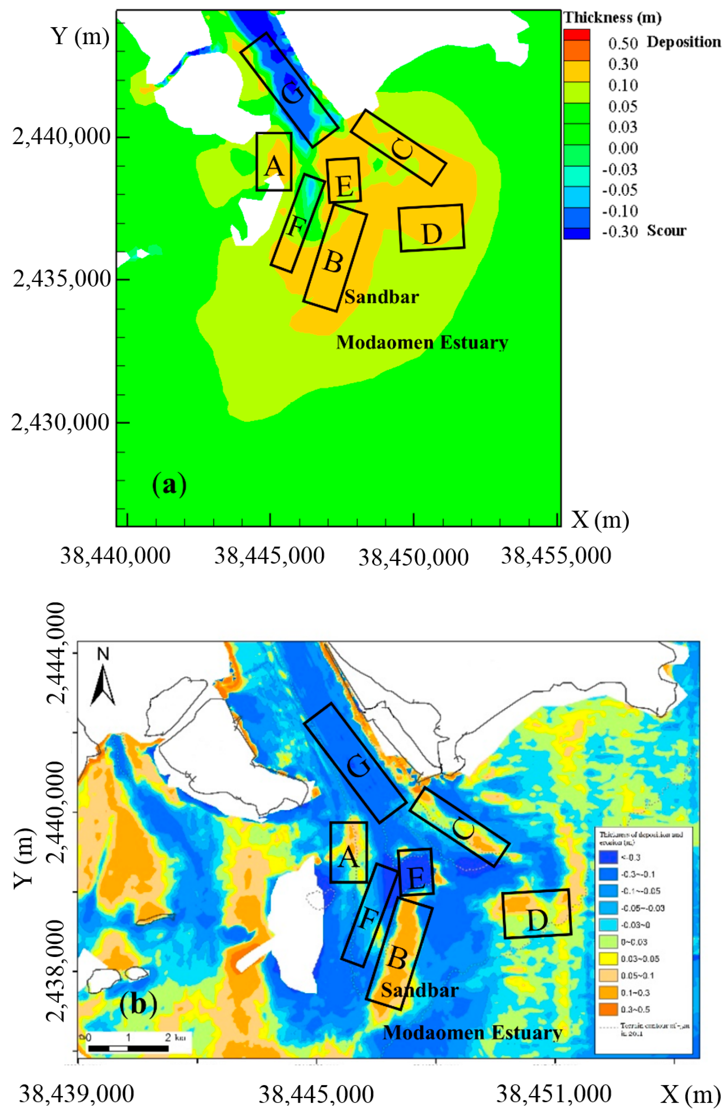
Figure 10a shows the simulated thickness of deposition and scour near the Modaomen Estuary; Figure 10b shows the annual average change of the measured terrain from 2005 to 2011. Figure 10c presents the 3D view of the measured terrain of the Modaomen Estuary in 2011. To compare the simulated thickness with the annual bed change, an amplification coefficient was used to compute the simulated thickness, i.e., the simulated thickness from the combined conditions of “99.7” was amplified by the coefficient. Since the net sediment transport during the “99.7” flood period was about 10% of the annual sediment transport through the Pearl River estuaries, the amplification coefficient was set to 10. To present quantitative comparison, we set seven blocks A–G in the Modaomen Estuary (see in Figure 10a,b). Table 1 presents the quantitative comparison of blocks A–G, from which it can be concluded that the simulated thickness of the deposition and scour in blocks A, B, C, D, G consist of the average change of the measured terrain from 2005 to 2011. However, due to human activity, namely sand extraction, block E was scoured, while the simulated results exhibited a deposition trend. Block F, which is the western branch (see in Figure 10c), was partially simulated by the proposed model. Besides, the eastern branch (see in Figure 10c) was not well simulated by the proposed model. The main reason for this is probably that the combined conditions of the “99.7” flood season are not adequately typical for the formation and evolution of the eastern branch. From Figure 10a it can be seen that there exists sediment deposition in the Modaomen Estuary, constructing a butterfly-shaped sandbar. Nevertheless, from Figure 10a,c it can be concluded that the butterfly shape of the sandbar was well simulated by the proposed model.
From Figure 10, it can be concluded that the formation and evolution process of the sandbar in the Modaomen Estuary is correctly simulated. The butterfly shape of sandbar in the Modaomen Estuary is considerably well simulated by the proposed model, which matches well with the measured terrain. The main reason for this would be that the combined conditions of the “99.7” flood season are typical for the formation and evolution of the sandbar.
As a whole, results show that the proposed model can accurately simulate the process of “wave-lifting-sand, tidal-current-transporting-sand” in the Lingding Sea, and the sandbar evolution process in Modaomen Estuary is well simulated.
6. Conclusions
In this work, a two-dimensional coupled tidal currents-waves-salinity-sediment model is proposed to simulate the sandbar evolution process in the Modaomen Estuary on an unstructured grid. The tidal currents, waves, and sediment are governed by the two-dimensional shallow water equations, the action density balance equation, and the advection-diffusion equation, respectively. To simulate the coupled effect between tidal currents and waves, the radiation stress of waves is considered in the source terms of the shallow water equation, and the effect of current on waves is computed by dynamically taking the water levels and velocities from the tidal current model to the wave model. An integrated solver is proposed for computing flow and sediment transport fluxes simultaneously, and then a two-dimensional coupled flow-sediment transport model based on unstructured Godunov-type scheme is developed. The MUSCL-Hancock scheme combined with the slope limiter is adopted to achieve the high-accuracy and high-resolution property. The effect of waves on sediment is considered by the sediment-carrying capacity and the condition of sediment incipient motion.
For the case study, the simulated result of sediment concentration distribution is in accordance with that of the actual situation in the Lingding Sea. The boundary of sediment concentration from Lingding shallows to Tonggu shallows is considerably well simulated. Besides, the butterfly shape of sandbar in the Modaomen Estuary is considerably well simulated by the proposed model, which matches well with the measured terrain. The performance of the proposed model is validated through an application to the case study of sandbar simulation in the Modaomen Estuary, China. The comparison between the simulated result and the measured terrain demonstrates that the complex coupling effects among tidal currents, waves, salinity and sediments are well simulated by the proposed model. So, it can be concluded that the proposed coupled numerical model can be used in the estuary regulation project, and thus has a bright application prospect. Since the finite-volume scheme used in this work is explicit, the computational time steps of the tidal currents model, salinity model, and sediment model are limited by the CFL condition, and the computational efficiency would be lower than the traditional implicit schemes if we use serial computation. To improve the computational efficiency of the proposed model, GPU-based high-performance computing method [34] will be used in the near future. Furthermore, the proposed morphodynamic model, which combines the SWAN model and Godunov-type tidal current model which uses the finite volume scheme as the solver, can be used to simulate the morphodynamic processes under sharp hydrodynamic gradients. It is worth assessing the sensibility of the proposed morphodynamic model under extreme hydrodynamic forcings [35,36].
Author Contributions
L.S. conceived the study; F.Y. designed the numerical experiments; H.W. performed the simulations; X.H. and H.W. analyzed the data and simulations; X.H. wrote the paper.
Funding
This research was funded by [National Key R&D Program of China] grant number [2017YFC0405900], [National Natural Science Foundation of China] grant number [51779280], [Science and Technology Special Funds Project of the Department of Water Resources of Guizhou Province] grant number [KT201606], and [Science and Technology Special Funds Project of the Department of Science and Technology of Guizhou Province: Qian Ke He Supporting] grant number [[2016]2561].
Acknowledgments
The authors are grateful to the anonymous reviewers for providing many constructive suggestions.
Conflicts of Interest
The authors declare no conflict of interest.
References
- Price, T.D.; Ruessink, B.G. State dynamics of a double sandbar system. Cont. Shelf Res. 2011, 31, 659–674. [Google Scholar] [CrossRef]
- Dubarbier, B.; Castelle, B.; Marieu, V.; Ruessink, G. Process-based modeling of cross-shore sandbar behavior. Coast. Eng. 2015, 95, 35–50. [Google Scholar] [CrossRef]
- Syed, Z.H.; Choi, G.; Byeon, S. A numerical approach to predict water levels in ungauged regions-case study of the Meghna River Estuary, Bangladesh. Water 2018, 10, 110. [Google Scholar] [CrossRef]
- Gallagher, E.L.; Steve, E.; Guza, R.T. Observations of sand bar evolution on a natural beach. J. Geophys. Res. Oceans 1998, 103, 3203–3215. [Google Scholar] [CrossRef]
- Ruessink, B.G.; Pape, L.; Turner, I.L. Daily to interannual cross-shore sandbar migration: Observations from a multiple sandbar system. Cont. Shelf Res. 2009, 29, 1663–1677. [Google Scholar] [CrossRef]
- Plant, N.G.; Todd, H.K.; Holman, R.A. A dynamical attractor governs beach response to storms. Geophys. Res. Lett. 2006, 33, 123–154. [Google Scholar] [CrossRef]
- Pape, L.; Kuriyama, Y.; Ruessink, B.G. Models and scales for cross-shore sandbar migration. J. Geophys. Res. Earth Surf. 2010, 115. [Google Scholar] [CrossRef]
- Ruessink, B.G.; Kuriyama, Y.; Reniers, A.J.H.M.; Roelvink, J.A.; Walstra, D.J.R. Modeling cross-shore sandbar behavior on the timescale of weeks. J. Geophys. Res. Earth Surf. 2007, 112. [Google Scholar] [CrossRef]
- Ruggiero, P.; Walstra, D.J.R.; Gelfenbaum, G.; Van Ormondt, M. Seasonal-scale nearshore morphological evolution: Field observations and numerical modeling. Coast. Eng. 2009, 56, 1153–1172. [Google Scholar] [CrossRef]
- Walstra, D.J.R.; Reniers, A.J.H.M.; Ranasinghe, R.; Roelvink, J.A.; Ruessink, B.G. On bar growth and decay during interannual net offshore migration. Coast. Eng. 2012, 60, 190–200. [Google Scholar] [CrossRef]
- Kuriyama, Y. Process-based one-dimensional model for cyclic longshore bar evolution. Coast. Eng. 2012, 62, 48–61. [Google Scholar] [CrossRef]
- Hayter, E.J.; Mehta, A.J. Modelling cohesive sediment transport in estuarial waters. Appl. Math. Model. 1986, 10, 294–303. [Google Scholar] [CrossRef]
- Jia, L.; Wen, Y.; Pan, S.; Liu, J.T.; He, J. Wave-current interaction in a river and wave dominant estuary: A seasonal contrast. Appl. Ocean Res. 2015, 52, 151–166. [Google Scholar] [CrossRef]
- Santoro, P.; Fossati, M.; Tassi, P.; Huybrechts, N.; Van Bang, D.P.; Piedra-Cueva, J.I. A coupled wave–current–sediment transport model for an estuarine system: Application to the Río de la Plata and Montevideo Bay. Appl. Math. Model. 2017, 52, 107–130. [Google Scholar] [CrossRef]
- Zhu, Z.N.; Wang, H.Q.; Guan, W.B.; Cao, Z. 3D numerical study on cohesive sediment dynamics of the Pearl River Estuary in the wet season. J. Mar. Sci. 2013, 31, 25–35. [Google Scholar]
- Yin, K.; Xu, S.; Huang, W. Modeling sediment concentration and transport induced by storm surge in Hengmen Eastern Access Channel. Nat. Hazards 2016, 82, 617–642. [Google Scholar] [CrossRef]
- Chen, X.H.; Chen, Y.Q.; Lai, G.Y. Modeling of the transport of suspended solids in the Estuary of Zhujiang River. Acta Oceanol. Sin. 2003, 25, 120–127. [Google Scholar]
- Song, L.; Zhou, J.; Guo, J.; Zou, Q.; Liu, Y. A robust well-balanced finite volume model for shallow water flows with wetting and drying over irregular terrain. Adv. Water Resour. 2011, 34, 915–932. [Google Scholar] [CrossRef]
- Dou, G.; Dong, F.; Dou, X.; Li, T. Research on mathematical model of estuarial and coastal sediment transport. Sci. China (Ser. A) 1995, 25, 995–1001. (In Chinese) [Google Scholar]
- The SWAN Team. SWAN Scientific and Technical Documentation (SWAN Cycle III Version 41.10); The SWAN Team: Delft, The Netherlands, 2016.
- Tan, G.; Fang, H.; Dey, S.; Wu, W. Rui-Jin Zhang’s research on sediment transport. ASCE J. Hydraul. Eng. 2018, 144, 02518002. [Google Scholar] [CrossRef]
- Richardson, J.F.; Zaki, W.N. Sedimentation and fluidization: Part I. Trans. Inst. Chem. Eng. 1954, 32, 35–53. [Google Scholar]
- Deng, J.; Deng, H. Study on Water-sediment Transport and River-bed Evolution at Pearl River Estuary. In Proceedings of the 5th International Conference on Estuaries and Coasts (ICEC-2015), Muscat, Oman, 2–4 November 2015. [Google Scholar]
- Dou, G.; Dong, F.; Dou, X. Sediment-laden capacity of tide and wave. J. Since Rep. 1995, 40, 443–446. (In Chinese) [Google Scholar]
- Wu, W.; Hu, C.; Yang, G. Two-dimensional horizontal mathematical model for flow and sediment. Chin. J. Hydraul. Eng. 1995. (In Chinese) [Google Scholar] [CrossRef]
- Song, L.; Zhou, J.; Li, Q.; Yang, X.; Zhang, Y. An unstructured finite volume model for dam-break floods with wet/dry fronts over complex topography. Int. J. Numer. Methods Fluids 2011, 67, 960–980. [Google Scholar] [CrossRef]
- Song, L.X.; Zhou, J.Z.; Wang, G.Q.; Wang, Y.C.; Liao, L.; Xie, T. Unstructured finite volume model for numerical simulation of dam-break flow. Adv. Water Sci. 2011, 22, 373–381. (In Chinese) [Google Scholar]
- Song, L.X.; Yang, F.; Hu, X.Z.; Yang, L.L.; Zhou, J.Z. A coupled mathematical model for two-dimensional flow-transport simulation in tidal river network. Adv. Water Sci. 2014, 25, 550–559. (In Chinese) [Google Scholar]
- Zhou, J.; Song, L.; Kursan, S.; Liu, Y. A two-dimensional coupled flow-mass transport model based on an improved unstructured finite volume algorithm. Environ. Res. 2015, 139, 65–74. [Google Scholar] [CrossRef] [PubMed]
- Zhou, Q.; Tian, L.; Wai, O.W.H.; Li, J.; Sun, Z.; Li, W. High-Frequency Monitoring of Suspended Sediment Variations for Water Quality Evaluation at Deep Bay, Pearl River Estuary, China: Influence Factors and Implications for Sampling Strategy. Water 2018, 10, 323. [Google Scholar] [CrossRef]
- Deng, J.; Ding, X. An analysis on the movement of the tide, sediment and salinity at the Pearl River Estuary. In Proceedings of the 4th International Conference on Estuaries and Coasts (ICEC-2012), Hanoi, Vietnam, 8–10 October 2012. [Google Scholar]
- Vinh, V.D.; Ouillon, S.; Thao, N.V.; Ngoc Tien, N. Numerical simulations of suspended sediment dynamics due to seasonal forcing in the Mekong coastal area. Water 2016, 8, 255. [Google Scholar] [CrossRef]
- Sadio, M.; Anthony, E.J.; Diaw, A.T.; Dussouillez, P.; Fleury, J.T.; Kane, A.; Almar, R.; Kestenare, E. Shoreline changes on the wave-influenced Senegal River Delta, West Africa: The roles of natural processes and human interventions. Water 2017, 9, 357. [Google Scholar] [CrossRef]
- Hu, X.; Song, L. Hydrodynamic modeling of flash flood in mountain watersheds based on high-performance GPU computing. Nat. Hazards 2018, 91, 567–586. [Google Scholar] [CrossRef]
- Gracia, V.; García, M.; Grifoll, M.; Sánchez-Arcilla, A. Breaching of a barrier under extreme events. The role of morphodynamic simulations. J. Coast. Res. 2013, 65, 951–956. [Google Scholar] [CrossRef]
- Sánchez-Arcilla Conejo, A.; Gracia, V.; García, M. Hydro morphodynamic modelling in Mediterranean storms: Errors and uncertainties under sharp gradients. Nat. Hazards Earth Syst. Sci. 2014, 2, 1693–1728. [Google Scholar] [CrossRef]
Figure 1.
The conceptual framework for model coupling.

Figure 2.
The sketch map of the study area (E1: Humen Estuary; E2: Jiaomen Estuary; E3: Hongqimen Estuary; E4: Hengmen Estuary; E5: Modaomen Estuary), and the upstream boundaries.
Figure 2.
The sketch map of the study area (E1: Humen Estuary; E2: Jiaomen Estuary; E3: Hongqimen Estuary; E4: Hengmen Estuary; E5: Modaomen Estuary), and the upstream boundaries.

Figure 3.
Computational grids, topography, and the tidal level boundaries of the study area.

Figure 4.
The spatial distribution of measuring points V1–V9.

Figure 5.
The comparison between the numerical results and the measured data: from 26 June 1998 20:00 to 27 June 1998 21:00. (a) The comparison between the computed and measured tidal levels; (b) The comparison between the computed and measured flow velocities and directions; (c) The comparison between the computed and measured sediment concentration.


Figure 6.
Sandbar simulation: the boundary conditions of the tidal currents model. (a) discharge (>0: ebb tidal; <0: flood tidal);(b) tidal level.
Figure 6.
Sandbar simulation: the boundary conditions of the tidal currents model. (a) discharge (>0: ebb tidal; <0: flood tidal);(b) tidal level.

Figure 7.
Sandbar simulation: boundary conditions of sediment concentration for the sediment model.

Figure 8.
Sandbar simulation: the distribution of (a) significant wave height and (b) wave period.

Figure 9.
Sandbar simulation: the distribution of sediment concentration (LS: Lingding shallows; TS: Tonggu shallows). (a) at flood fast tide; (b) at ebb fast tide.
Figure 9.
Sandbar simulation: the distribution of sediment concentration (LS: Lingding shallows; TS: Tonggu shallows). (a) at flood fast tide; (b) at ebb fast tide.


Figure 10.
The sandbar in Modaomen Estuary. (a)The simulated thickness of deposition and scour; (b) The annual average change of the measured terrain from 2005 to 2011; (c) The measured terrain in 2011.
Figure 10.
The sandbar in Modaomen Estuary. (a)The simulated thickness of deposition and scour; (b) The annual average change of the measured terrain from 2005 to 2011; (c) The measured terrain in 2011.


Table 1.
The quantitative comparison of blocks A–G: simulated thickness of deposition and scour vs. annual average change of measured terrain from 2005 to 2011. (unit: m; positive: deposition; negative: scour).
Table 1.
The quantitative comparison of blocks A–G: simulated thickness of deposition and scour vs. annual average change of measured terrain from 2005 to 2011. (unit: m; positive: deposition; negative: scour).
| Blocks | A | B | C | D | E | F | G |
|---|---|---|---|---|---|---|---|
| Simulated | 0.1~0.3 | 0.1~0.3 | 0.1~0.3 | 0.1~0.3 | 0.1~0.3 | −0.05~0.3 | −0.3~−0.1 |
| Measured | 0.05~0.3 | 0.1~0.3 | 0.03~0.3 | 0.03~0.3 | <−0.3 | −0.3~−0.05 | −0.3~−0.1 |
© 2018 by the authors. Licensee MDPI, Basel, Switzerland. This article is an open access article distributed under the terms and conditions of the Creative Commons Attribution (CC BY) license (http://creativecommons.org/licenses/by/4.0/).
Share and Cite
MDPI and ACS Style
Hu, X.; Yang, F.; Song, L.; Wang, H. An Unstructured-Grid Based Morphodynamic Model for Sandbar Simulation in the Modaomen Estuary, China. Water 2018, 10, 611. https://doi.org/10.3390/w10050611
AMA Style
Hu X, Yang F, Song L, Wang H. An Unstructured-Grid Based Morphodynamic Model for Sandbar Simulation in the Modaomen Estuary, China. Water. 2018; 10(5):611. https://doi.org/10.3390/w10050611
Chicago/Turabian StyleHu, Xiaozhang, Fang Yang, Lixiang Song, and Hangang Wang. 2018. "An Unstructured-Grid Based Morphodynamic Model for Sandbar Simulation in the Modaomen Estuary, China" Water 10, no. 5: 611. https://doi.org/10.3390/w10050611
Note that from the first issue of 2016, this journal uses article numbers instead of page numbers. See further details here.