Impact of the Storm Sewer Network Complexity on Flood Simulations According to the Stroke Scaling Method


1
Key Laboratory of Virtual Geographic Environment, Nanjing Normal University, Ministry of Education, Nanjing 210023, China
2
Water and Environmental Management Research Centre, Department of Civil Engineering, University of Bristol, Bristol BS8 1TR, UK
3
Jiangsu Center for Collaborative Innovation in Geographical Information Resource Development and Application, Nanjing 210023, China
*
Authors to whom correspondence should be addressed.
Water 2018, 10(5), 645; https://doi.org/10.3390/w10050645
Submission received: 18 April 2018
/
Revised: 12 May 2018
/
Accepted: 15 May 2018
/
Published: 16 May 2018
(This article belongs to the Section Urban Water Management)
Abstract
:For urban watersheds, the storm sewer network provides indispensable data for flood modeling but often needs to be simplified to balance the conflict between the large amount of data and current computing power. The sensitivity of a flood simulation to the data precision of a storm sewer network needs to be explored to develop reasonable generalization strategies. In this study, the impact of using the stroke scaling method to generalize a storm sewer network on a flood simulation was analyzed in terms of the total inflow of the outfalls and flood results. The results of the three study basins showed that different complexities of a sewer network did not have a significant effect on the outfall’s total inflow for an area with a single drainage system but did for an area with multiple drainage systems. In addition, serious flooding was mainly distributed at the backbone pipes, which can be identified with the simplified sewer network. Several effective generalization strategies were developed for sewer networks that consider the distribution characteristics of the drainage system and application requirements. This study is theoretically important for better understanding the data sensitivity of flood modeling and simulation and practically important for improving the modeling efficiency and the accuracy of urban flood simulation.
1. Introduction
Because of global climate change and accelerating urbanization, extreme weather events—especially extreme precipitation and flood hazards—are becoming increasingly frequent and serious. They are a major global problem facing humans [1,2]. There are several engineering and non-engineering measures for dealing with heavy rainfall and flood hazards by predicting, preventing, and alleviating the effects of urban floods on urban systems to some extent [3]. Among them, non-engineering measures against flood hazards frequently use the simulated and predicted results of hydrologic models [4,5,6].
However, flood modeling and simulation are more challenging for urban areas than rural areas because of the higher requirements for input data, the more complex simulation of the drainage system, and the more sophisticated exchange between surface and groundwater flows [7,8,9]. In particular, the quantity and quality of data are significant factors that limits the accuracy of urban flood simulations [10,11,12,13]. Because of the high non-permeability of urban surfaces, storm runoff that cannot infiltrate underground is mainly discharged into rivers through the storm sewer network [14,15,16]. Therefore, the quantity and quality of data on the storm sewer system are indispensable for flood simulation.
Given the limits of data availability and current computing power, simplified or low-precision data are usually used for urban hydrologic modeling. However, low-precision data may reduce the accuracy of the flood simulation. Many studies in the literature have used multiscale data to examine the impact of the data precision or resolution on the accuracy or sensitivity of flood modeling and simulation [17,18,19]. Some researchers have investigated the influence of different resolutions of topographic data on the simulation results of hydrologic models [19,20,21,22,23]. For example, Chaubey et al. [21] evaluated the effect of the digital elevation model (DEM) resolution on the output uncertainty of the Soil and Water Assessment Tool (SWAT) model in seven scenarios and found that the DEM resolution affects the model in terms of watershed delineation, the stream network, and sub-basin classification. Several studies have also explored the effect of the degree of aggregation on hydrologic simulations by varying the number of watershed subdivisions [17,18,24]. For example, Cleveland et al. [17] simulated runoff with the Hydrologic Modeling System (HEC-HMS) and discovered that the size or number of sub-watersheds have little influence on the computed runoff hydrographs. Carpenter et al. [25] studied the effects of model parameters and precipitation uncertainty on streamflow simulations of a distributed hydrologic model, and Yu et al. [9] explored the effect of hydrologic parameters for a catchment on urban surface water flooding based on a hydro-inundation model.
For urban watersheds, it is also important to explore the effect of the degree of generalization for a storm sewer network on the accuracy or sensitivity of the flood modeling and simulation [26,27,28]. Park et al. [28] investigated the spatial resolution of the sewer network on the Storm Water Management Model (SWMM) and found that it did not have a significant effect on the simulated runoff volume. Krebs et al. [27] demonstrated that, while the runoff volume is almost unaffected by the spatial resolution of a sewer network, lower resolutions lead to the overestimation of peak flow because of the excessively rapid catchment response to storm events. Ghosh et al. [26] examined actual and artificial drainage networks and found that peak flows show a dual-scale effect, where aggregation reduces peak flows for larger storms and increases them for smaller storms.
However, most related studies have not explored the driving mechanism of the complexity of urban storm sewers on the results of hydrologic models. In addition, there has been little research on developing efficient or automatic generalization methods for storm sewer network, even though this process is necessary to improve the simulation efficiency. The degree of generalization or approach can differ depending on the precision requirements, topographic features, and so on. Thus, different generalization strategies or methods need to be developed for different application requirements, regional features, or structural characteristics of storm sewers while finding a balance between the simulation accuracy and efficiency.
The objectives of this study were as follows: (1) design an automatic and high-efficiency method for storm sewer network generalization; (2) explore the impact of urban drainage system complexity on flooding simulation by using multiple basins with different drainage system structures and summarize the laws and driving mechanisms for the flood simulation sensitivity induced by the spatial resolution of the sewer network; and (3) propose different generalization methods of the storm sewer network for different application purposes, geographic features, and drainage structures.
2. Methodology
2.1. Storm Water Management Model
The open source hydrologic model (the SWMM), which was developed by the US Environmental Protection Agency [29], was selected as the modeling platform for flood simulation in this study. The SWMM is a 1D dynamic rainfall-runoff simulation model for urban watersheds and combined sewer overflow phenomena [30]. The main implementation principles and ideas fully consider the features of the urban watershed environment [29]. The SWMM includes four calculation modules: flow generation, transport, extended delivery, and storage/processing. These are used to simulate the surface water production and sinking of urban watersheds, storm sewer network convergence, and water storage and sewage treatment processes [29]. The rainfall–runoff produced in subcatchments flows into the storm sewer network through manholes and combines with dry-weather flow and ground-water infiltration [30]. Flow routing from upstream and downstream boundaries of the storm sewer system is governed by the conservation of mass and momentum equations for gradually varied, turbulent, and unsteady flow (Saint Venant) equations [30,31]. For more details, see [30]. For overland flooding simulations with SWMM, the excess volume of overflow junctions flows evenly into a ponded area that can be set to the area within the subcatchment that can be flooded (subtracting the building footprint) [29].
In this study, flow routing was computed according to dynamic wave theory and infiltration based on the Green–Ampt method [27]. For the main estimation procedure, the measured parameters [32,33] (e.g., area, width, and slope) are based on measurement and spatial analysis technologies with a geographic information system (GIS) [34,35], and the inferred parameters [32,33] (e.g., roughness coefficients) are based on empirical estimation [35]. Parameters are calibrated and verified by trial and error with an automatic optimization procedure, where the objective is to maximize the Nash–Sutcliffe (NS) coefficient of efficiency likelihood values. Details are presented in [35].
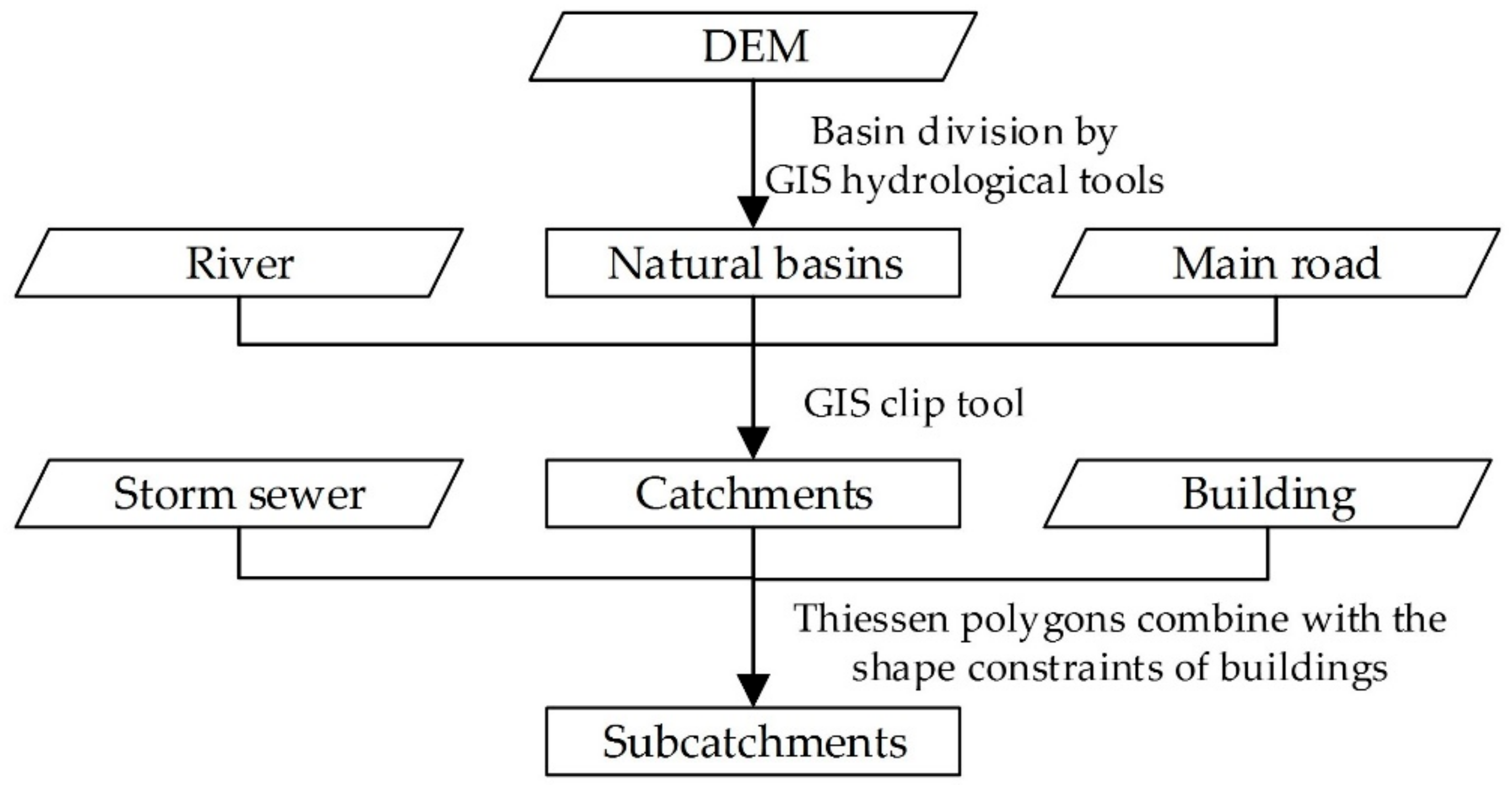
The catchment discretization procedure [36] is mainly based on [34] and [35] and uses GIS technology to fully consider various factors that affect the flow process of a city’s water flow, including rivers, roads, storm sewer networks, and buildings. As shown in Figure 1, DEM data are first used to analyze the flow paths of urban surface water and obtain the natural basins with GIS hydrologic tools [34,37]. Second, given that rivers and main roads obstruct rainfall across themselves, the centerlines of rivers and main roads are applied to split natural basins into catchments with the GIS clip tools. Finally, the catchments are divided into subcatchments based on the Thiessen polygon method to help assign rainfall data from each rain gage to the nearest subcatchment [38,39]. The shapes of subcatchments are then revised by considering the effect of buildings on the direction of storm runoff.
2.2. The Stroke Scaling Method
The main approach to expressing a storm sewer network is based on the node–arc structure. This structure separates conduits and has poor visual coherence, which makes it difficult to match a human’s overall perception. Moreover, the large number of junctions and conduits in the storm sewer network result in inefficient or low accuracy of the generalization or classification method, even within a small area. Therefore, we used the stroke technique [40,41,42] to design a stroke scaling method for simplifying and classifying a storm sewer network in a highly efficient and accurate manner.
The stroke technique concatenates separate line segments (e.g., conduits) into longer lines to detect and resolve spatial inconsistencies [40,41,42]; this provides a more integrated structure to further improve the efficiency of subsequent processing. During the generalization procedure for a storm sewer network, we usually keep or remove conduits and connected junctions with similar shapes or attributes. For example, we may remove conduits with a diameter of less than 400 cm or that are not laid on the main roads. Therefore, we can consolidate the connectivity of conduits with similar shapes or attributes into one pipe stroke to simplify the structure of the storm sewer network and improve the later processing speed.
The main idea of pipe stroke construction is to convert L conduits into S pipe strokes () based on certain constraints. This can be expressed as follows:
where is all conduits of the storm sewer network, is the number of conduits, represents all pipe strokes of the storm sewer network, is the number of all pipe strokes, and is one of .
We select the angle () between conduits and the horizontal direction, the road level () that the conduits are laid on, and the diameter () of the conduit as constraints for combining two conduits () that are directly connected to each other into one pipe stroke. The following conditions need to be met:
where is the difference threshold between the values of and , and is the difference threshold between the values of and . The values of and depend on the shape and attribute characteristics of the sewer network in the study area.
For convenient generalization or classification of the sewer network, in addition to the conduits, we also add the junction information, start the search junction, and the level of the pipe stroke. Thus, the pipe stroke comprises all of the information of the original components but with more integrity. The data structure of the pipe stroke can be described as follows:
where PS is the pipe stroke, L is the set of conduits of the pipe stroke, P is the set of junctions of the pipe stroke, StartP is the start search junction of the pipe stroke, and Le is the level of the pipe stroke. The level is assigned according to the distance from the pipe stroke to the outfall. The level of the pipe stroke () that is directly connected to the outfall is set to 1, the level of the pipe stroke that is directly connected to is set to 2, and so on. We also set Le of the pipe stroke at the end of the sewer network and the total length to be less than a given threshold, which depends on the actual situation at the last level. This ensures that the unimportant segments are deleted during the generalization procedure.
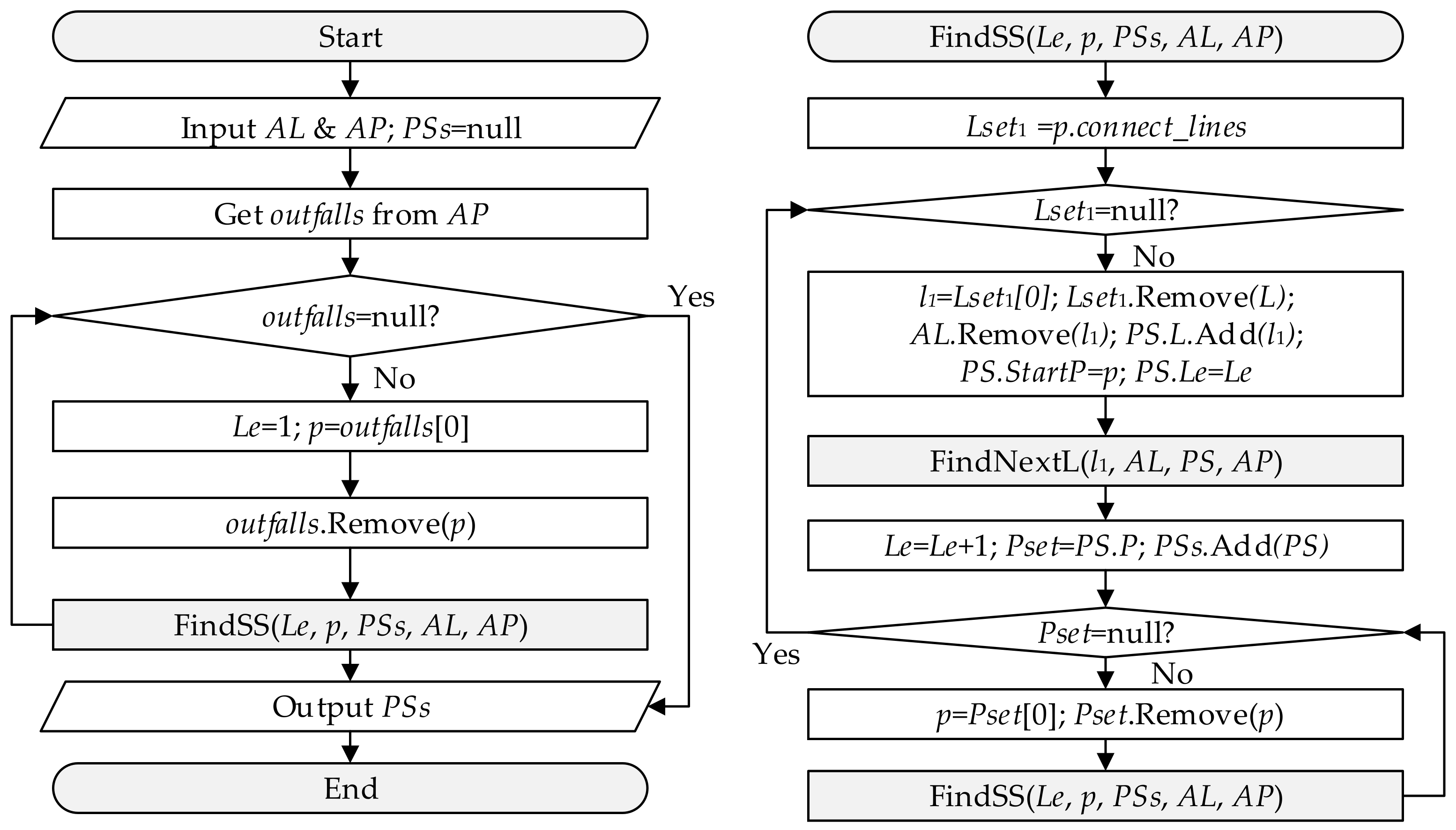
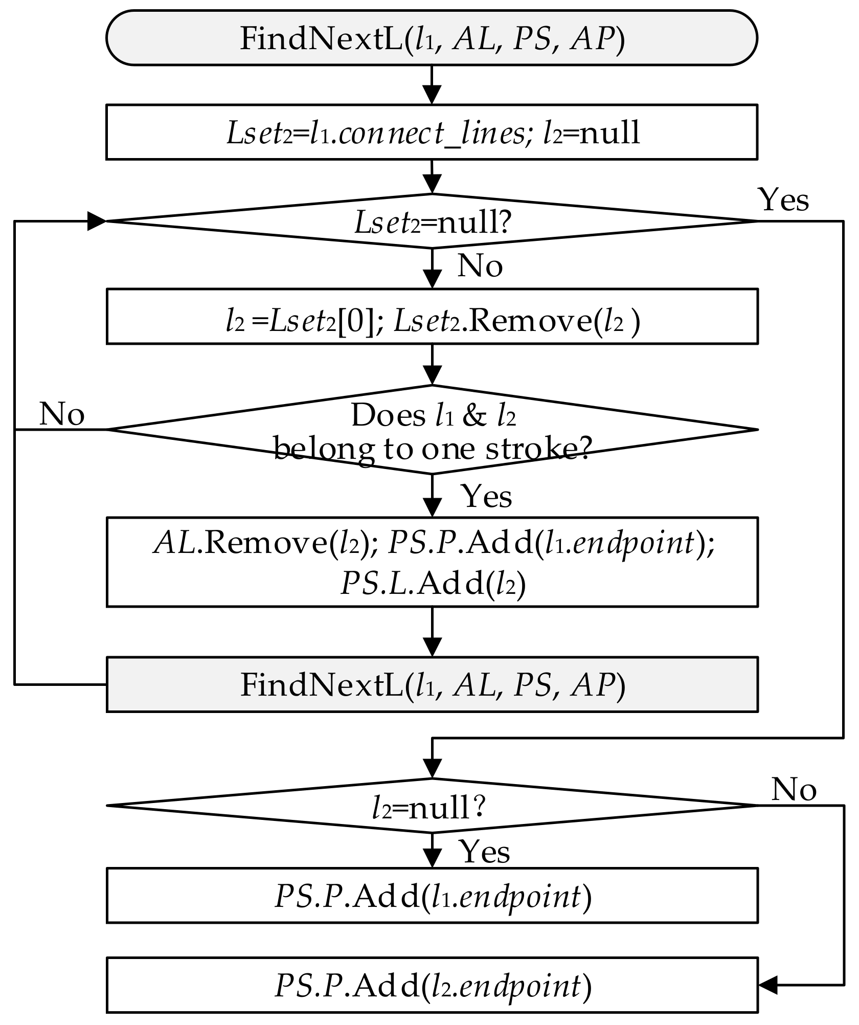
The complete construction algorithm of pipe strokes is displayed in Figure 2 and Figure 3. PSs are the set of all pipe strokes of the storm sewer network. AL and AP represent the shape and attribute information of all conduits and junctions of the original storm sewer network. Lset1 represents the conduits that connect to StartP directly from the set of all conduits (AL). Lset2 represents the conduits that connect to l1 directly from the set of all conduits (AL). Pset is P of the PS for which construction was just finished. FindSS() is the function for searching the pipe strokes set of the original sewer network. FindNextL() is the function of finding the next conduit and junction of a pipe stroke. The main idea of this algorithm is to proceed from the outfall to the upstream pipes to find each pipe stroke and assign Le to strokes based on the upstream and downstream relationships of the storm sewer network (i.e., function FindSS()), as shown in Figure 2. The main idea of the construction algorithm for each pipe stroke is to start from the given junction, which is set as StartP, and then select one conduit that connects with StartP directly as the seed conduit (l1). Then, a traversal search is performed for all conduits (L) and other junctions (P) that belong to this pipe stroke based on the connectivity between conduits and the constraints (Equations (5)–(7)) to determine whether two conduits belong to one pipe stroke (i.e., function FindNextL()), as shown in Figure 3.
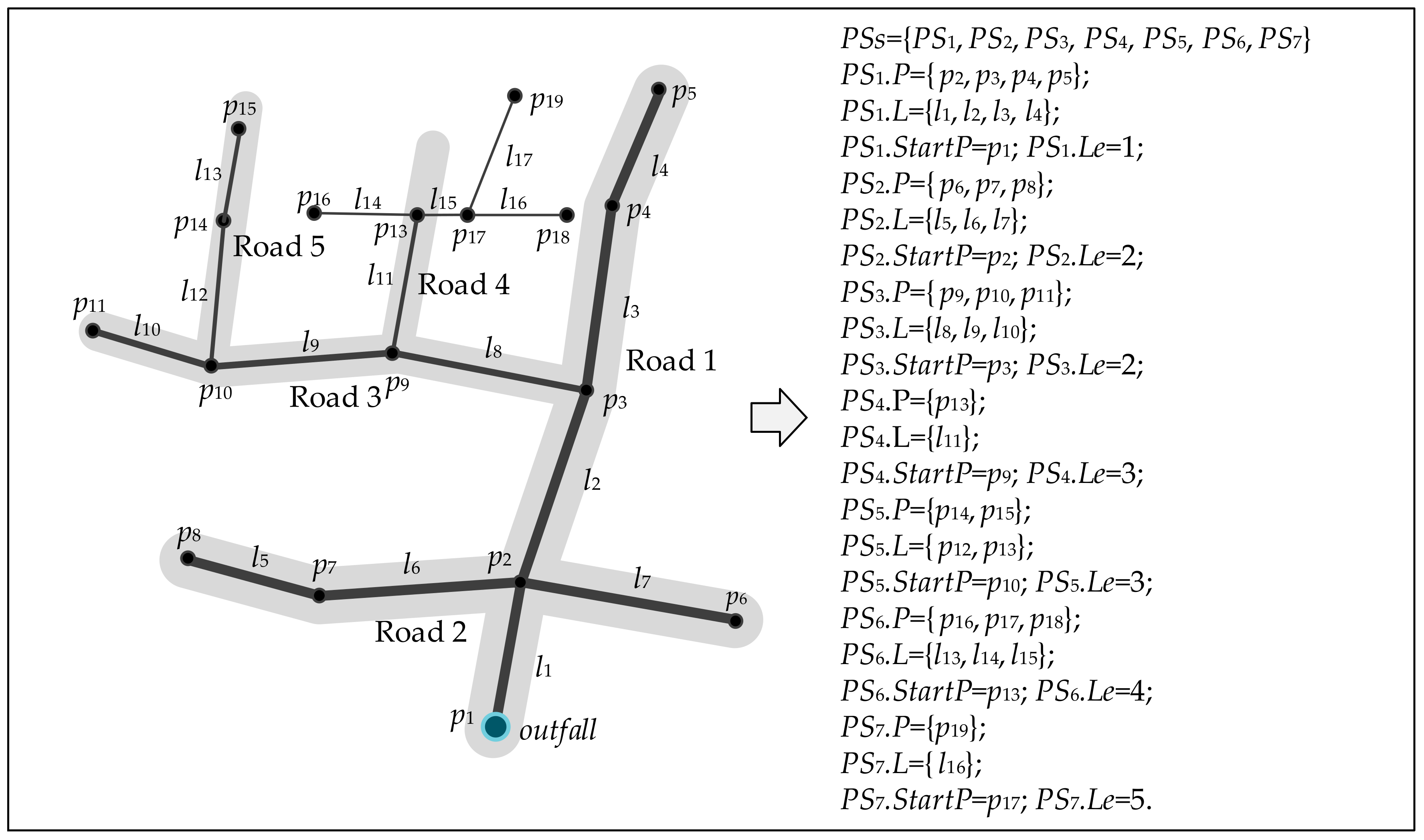
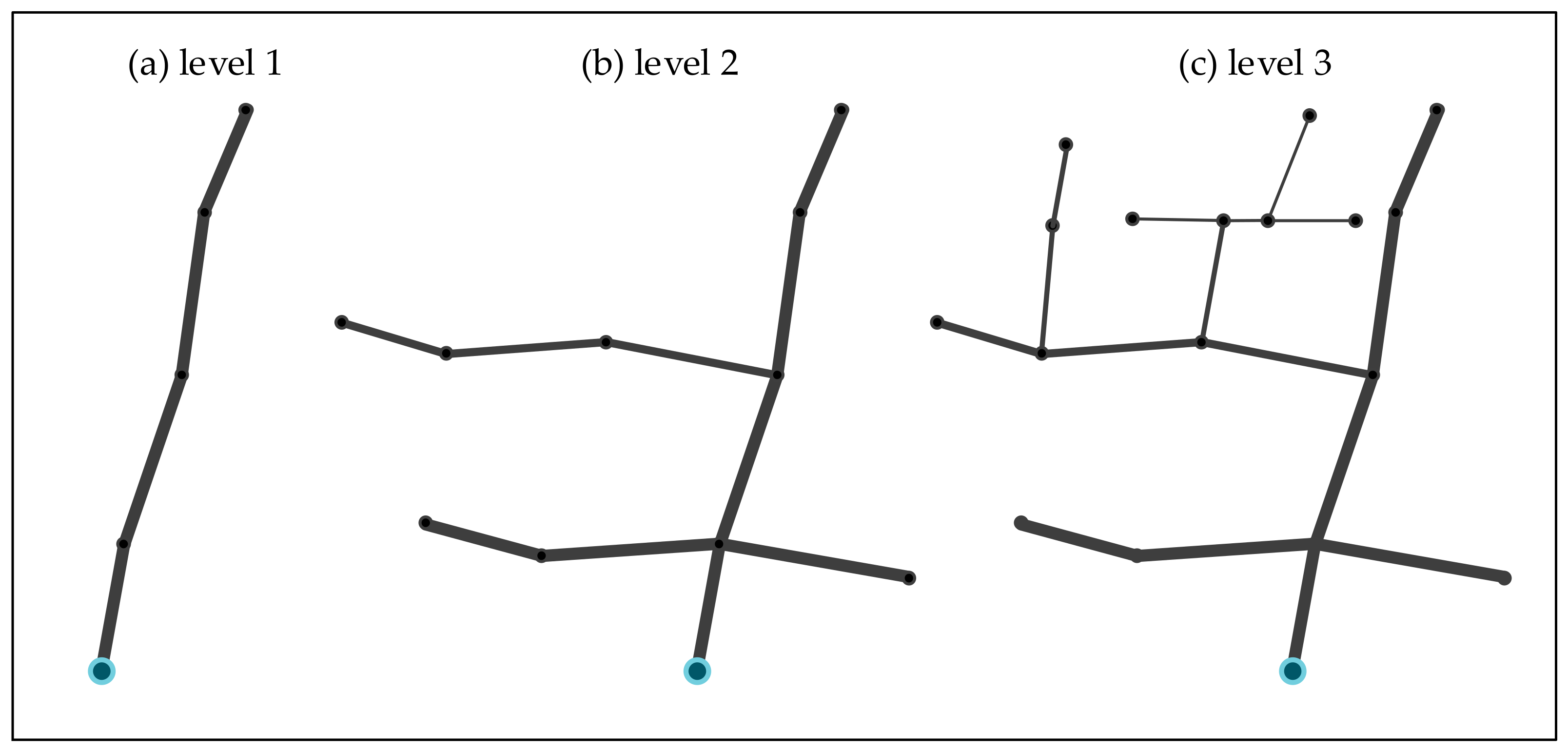
Figure 4 shows a simple example to explain the pipe stroke construction method and the corresponding classification results. The sewer network in this figure with conduits l1, l2, …, l17 and junctions p1, p2, …, p19 is spread on five roads (Roads 1–5). The pipe diameters of l1, l2, l3, l4, l5, l6, and l7 are 0.8 m; the pipe diameters of l8, l9, and l10 are 0.6 m; and the diameters of other pipes are 0.4 m. We set = 50° and = 0.3 m based on the sewer network shape shown on the left side of Figure 4 and the pipe diameter of each pipeline. We can get seven pipe strokes (PS1–PS7) based on the algorithm of the pipe stroke construction (Figure 2). The right side of Figure 4 displays the P, L, StartP, and Le of each stroke. As shown in Figure 5, we can divide the structure of the pipe system into three levels from simple to complex. Leve1 1 contains PS1; Level 2 contains PS1, PS2, and PS3; Level 3 contains PS1, PS2, PS3, PS4, PS5, PS6, and PS7.
3. Study Area and Scenario Design
3.1. Study Area
Nanjing is one of the biggest cities in China, and its terrain is dominated by low hills. Its main water system comes from the Yangtze River and three urban rivers: the Moat, the Qinhuai River, and the Jinchuan River. In the rainy season, the city is frequently hit by extreme precipitation; this, combined with the increasing imperviousness and low capacity of the drainage system, results in waterlogging or flood hazards. Heavy rainfall-driven hazards cause shutdowns of the traffic system, inconvenient travel, building damage, and so on; thus, they have become a significant factor affecting the socioeconomic development of Nanjing.
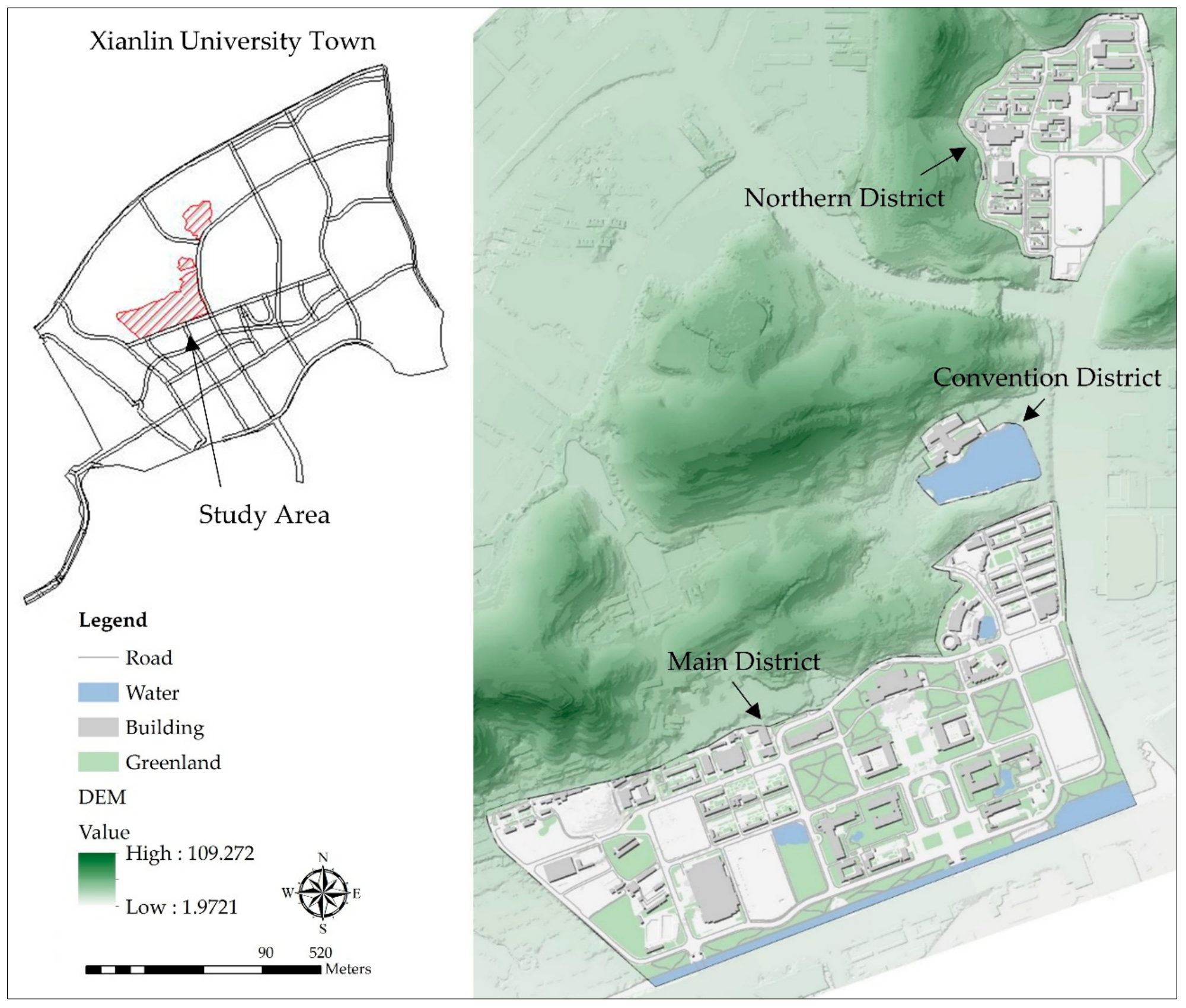
Nanjing Normal University is located in the northeast of the city and belongs to an area where mountains meet the plains. The terrain of the campus is undulating and complex. We selected the campus of Nanjing Normal University as a study area to identify the impact of urban drainage system complexity on flood simulation. We divided the study area into three sub-basins: the northern district, the convention district, and the main district. These sub-basins have different terrain characteristics and distributions of the construction area, as shown in Figure 6. The drainage systems of these sub-basins are isolated because of walls, roads, and cutoff ditches at their boundaries. The walls and roads obstruct the exchange of water from the sub-basins and outside, and the cutoff ditch prevents the inflow of storm runoff from the hillsides into the sub-basins.
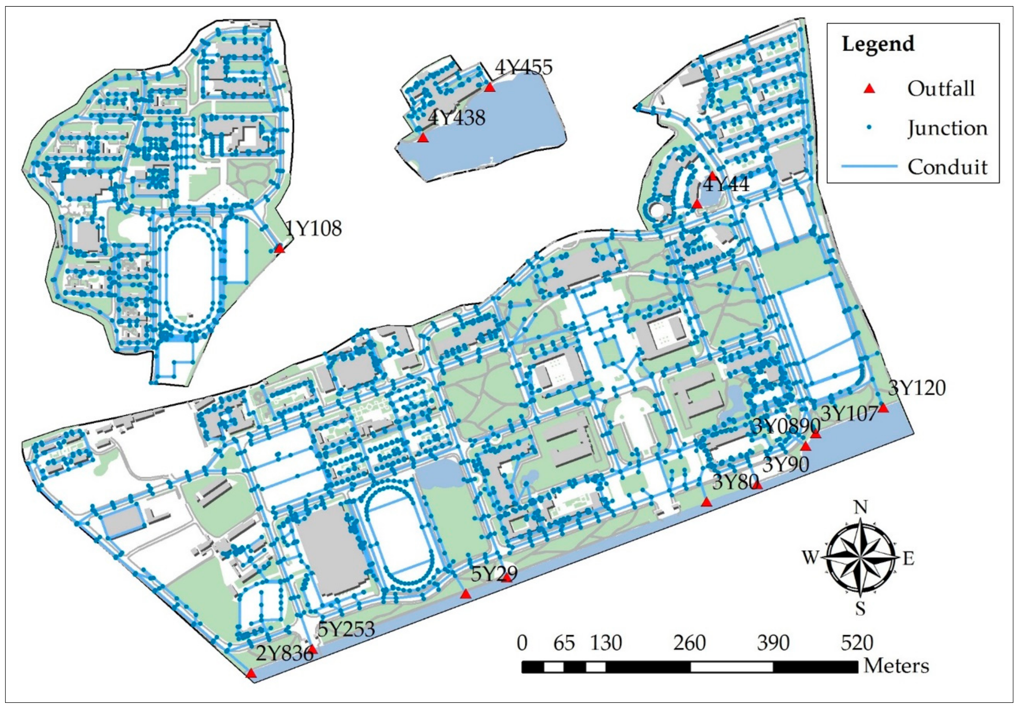
In this study, the main datasets included DEM data with a resolution of 1 m for rivers, buildings, green land, roads, and the storm sewer network. As listed in Table 1, the area, impermeability, total conduit length, and numbers of junctions and outfalls were 15.83 ha, 70.84%, 9.15 km, 1057, and 1, respectively, for the northern district; 3.47 ha, 28.56%, 0.60 km, 97, and 2, respectively, for the convention district; and 60.00 ha, 64.62%, 26.22 km, 2701, and 11, respectively, for the main district. Figure 7 shows the distribution of the storm sewer networks for the three sub-basins. One drainage system discharges rainwater into the drainage system outside the campus through outfall 1Y108 in the northern district, two drainage systems discharge into the lake through outfalls 4Y438 and 4Y455 in the convention district, and 11 drainage systems discharge into the river in the main district.
3.2. Scenario Design
In order to consider the structure and complexity of the storm sewer system in the study area, we classified the networks in the three sub-basins (northern district, convention district, and main district) into four levels (1–4) based on the stroke scaling method presented in Section 2.2. The complexity of the sewer network increased from Level 1 to Level 4. The four levels of the sewer network were combined with the DEM, rivers, buildings, green land, and roads dataset for four subdivisions (1–4) based on the catchment discretization techniques described in Section 2.1.
We constructed Chicago design storms [43,44] with four different return periods (2, 10, 50, and 100 years) with a rainfall duration of 2 h based on the following Nanjing storm intensity equation, which was derived from local rainfall records for more than 60 years:
where i is the rainfall intensity (mm/min), t is the rainfall duration (min), and p is the return period (year) of the rainfall event. We chose a rainfall duration of 2 h for the modeling and simulation because the Chicago hyetograph with a rainfall duration of 2 h is considered an appropriate way to simulate extreme rainfall in China [45,46]. The error would increase if a storm longer than 2 h was simulated [45,46].
Therefore, we designed 16 scenarios for the three sub-basins, as listed in Table 2. S4, S8, S12, and S16 were control groups for the sewer network in scenarios that were not simplified, and the rest of the scenarios were experimental groups.
4. Results and Discussion
4.1. Classification and Discretization Results
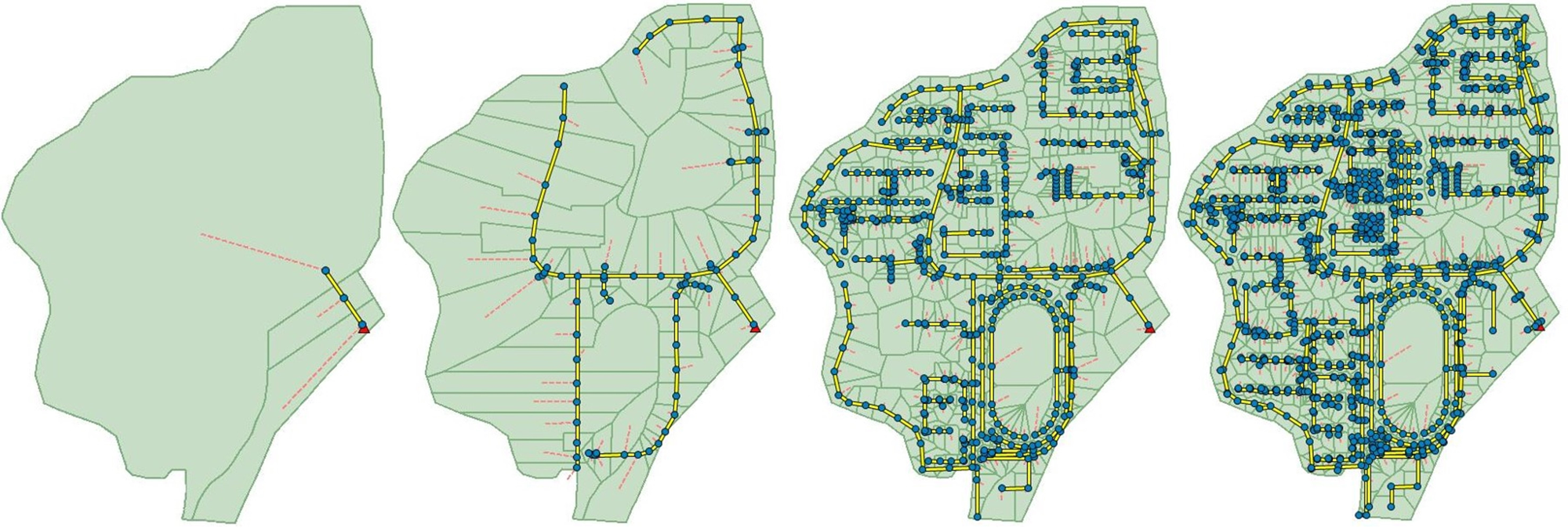
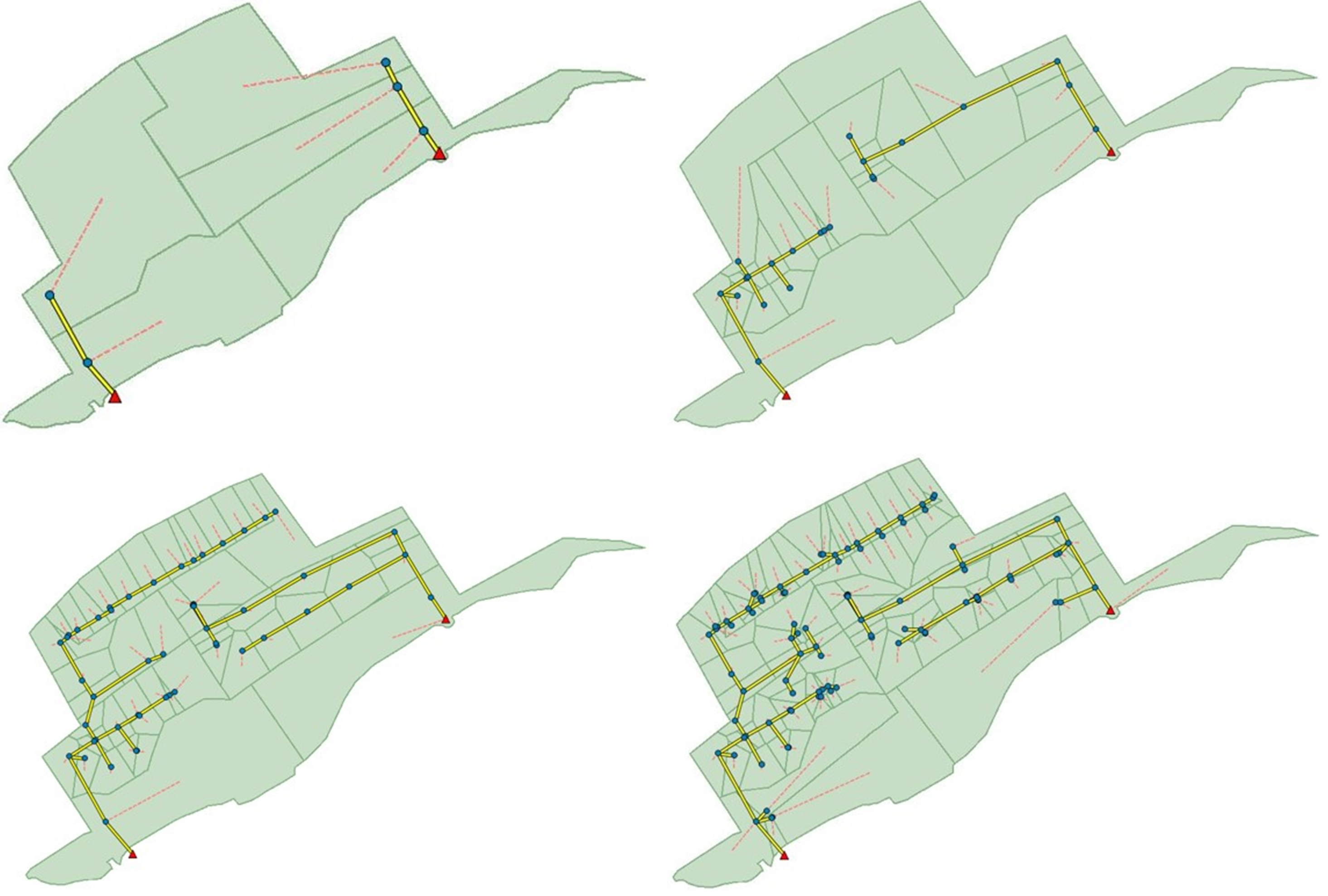
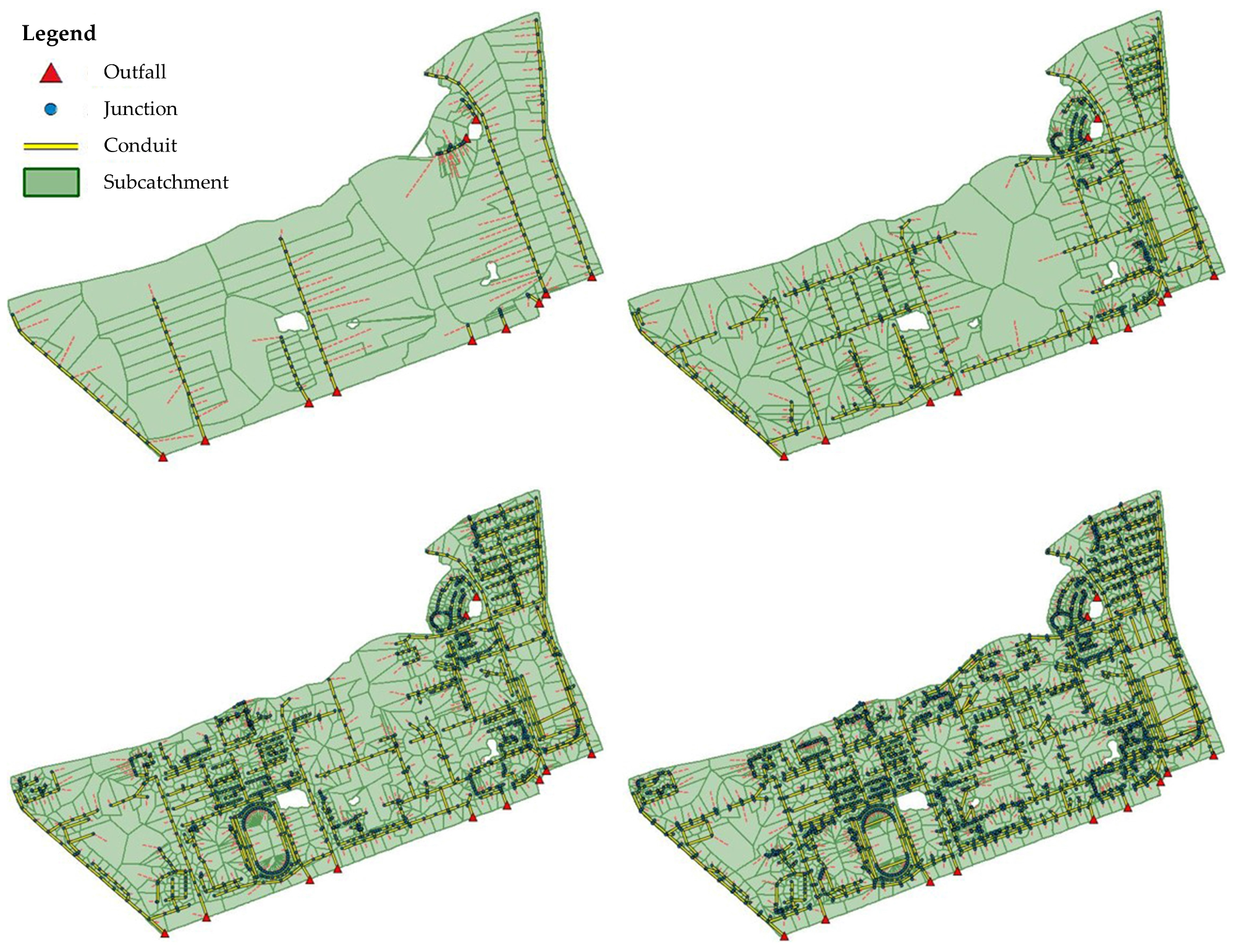
Figure 8, Figure 9 and Figure 10 display the classification results for the four complexity levels of the storm sewer networks and corresponding discretization results for the three sub-basins. For the northern district, the total conduit lengths at Levels 1–4 were 0.08, 1.54, 6.58, and 9.15 km, respectively; this corresponded to 3, 79, 531, and 1055 subcatchments, respectively. For the convention district, the total conduit lengths were 0.07, 0.23, 0.43, and 0.60 km, which corresponded to 5, 22, 47, and 96 subcatchments, respectively. For the main district, the total conduit lengths were 2.90, 9.80, 18.70, and 27.00 km, which corresponded to 114, 519, 1336, and 2717 subcatchments, respectively. The details are presented in Table 3.
The Level 1 sewer network only contained the pipe stroke with StartP as the outfall; it covered one part of the main roads of the study area. The Level 2 sewer network covered almost all of the main roads of the study area. The complexity of the Level 3 network was between those of Level 2 and the original sewer network (Level 4).
4.2. Results of Outfalls’ Total Inflow
We built and modeled the SWMMs for 16 scenarios (S1–S16) based on the classification and discretization results for the three sub-basins. We then ran the models to obtain 16 flood simulation results for each sub-basin. Table 4 displays the cost time for simulating the four kinds of storm sewer network with different levels of complexity for the storm with a 50-year return period. The simulation times with the other return periods were similar. Unsurprisingly, the simulation time significantly increased with the complexity of the pipe network, which means that simplifying the sewer network can obviously improve the simulation speed.
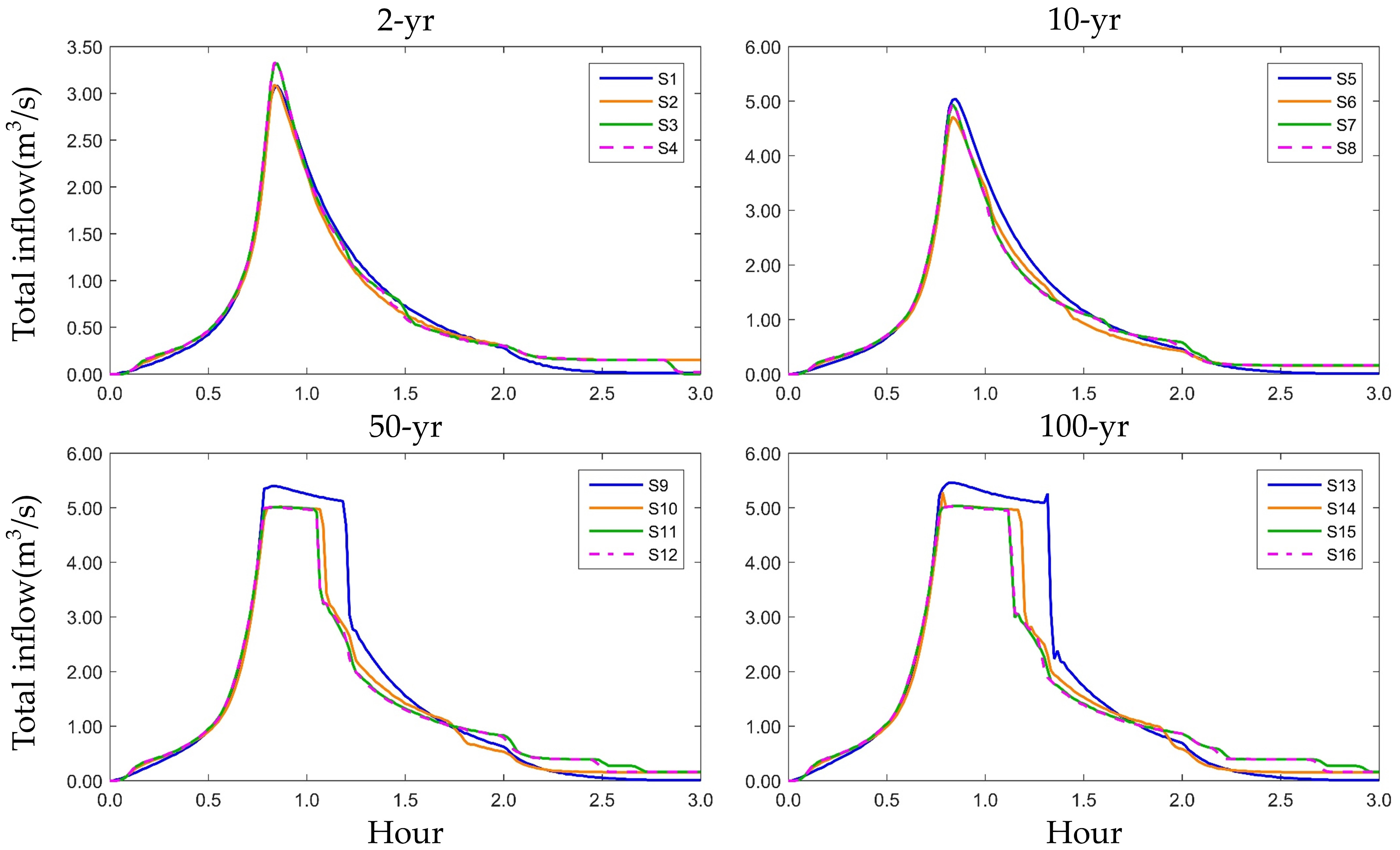
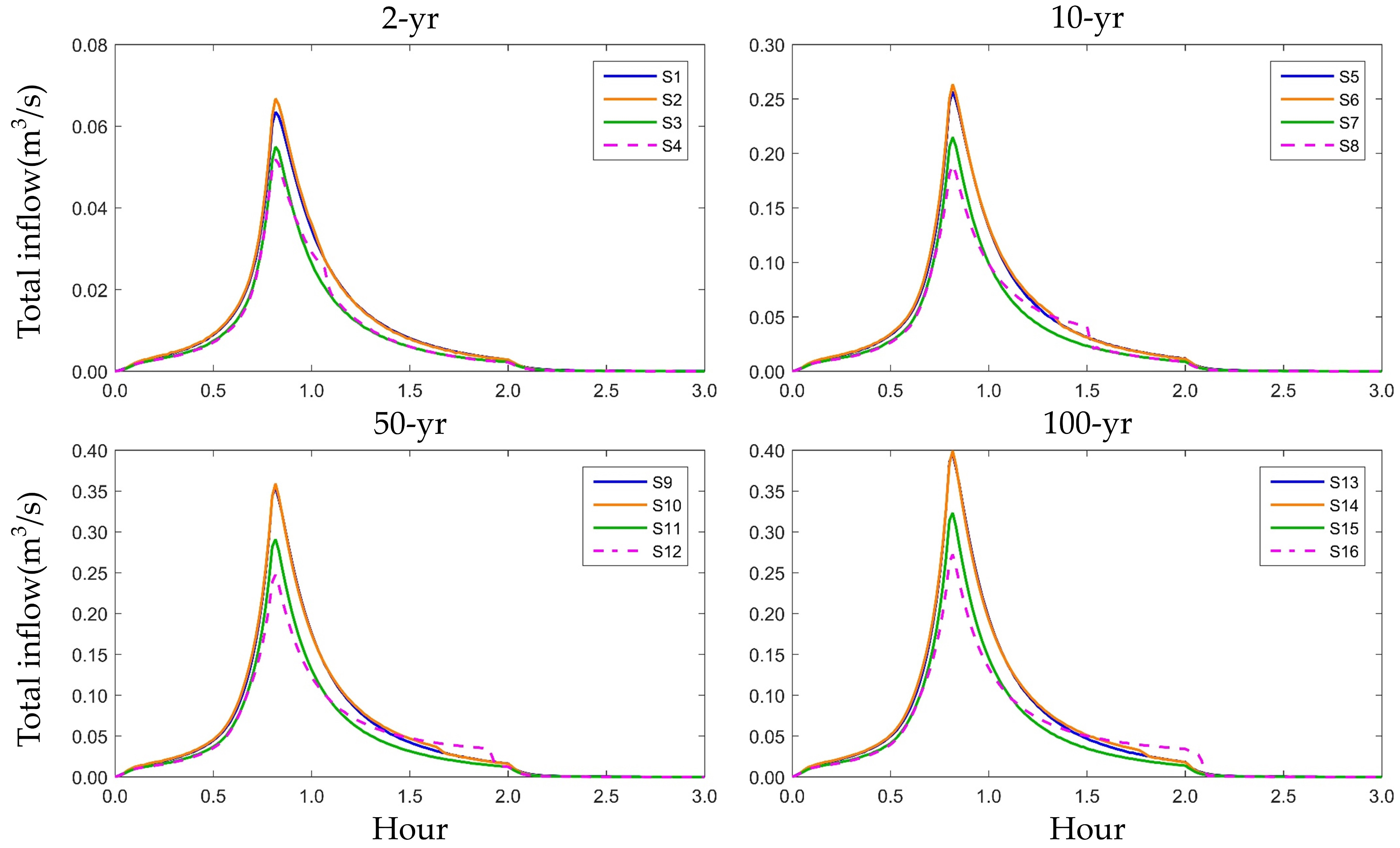
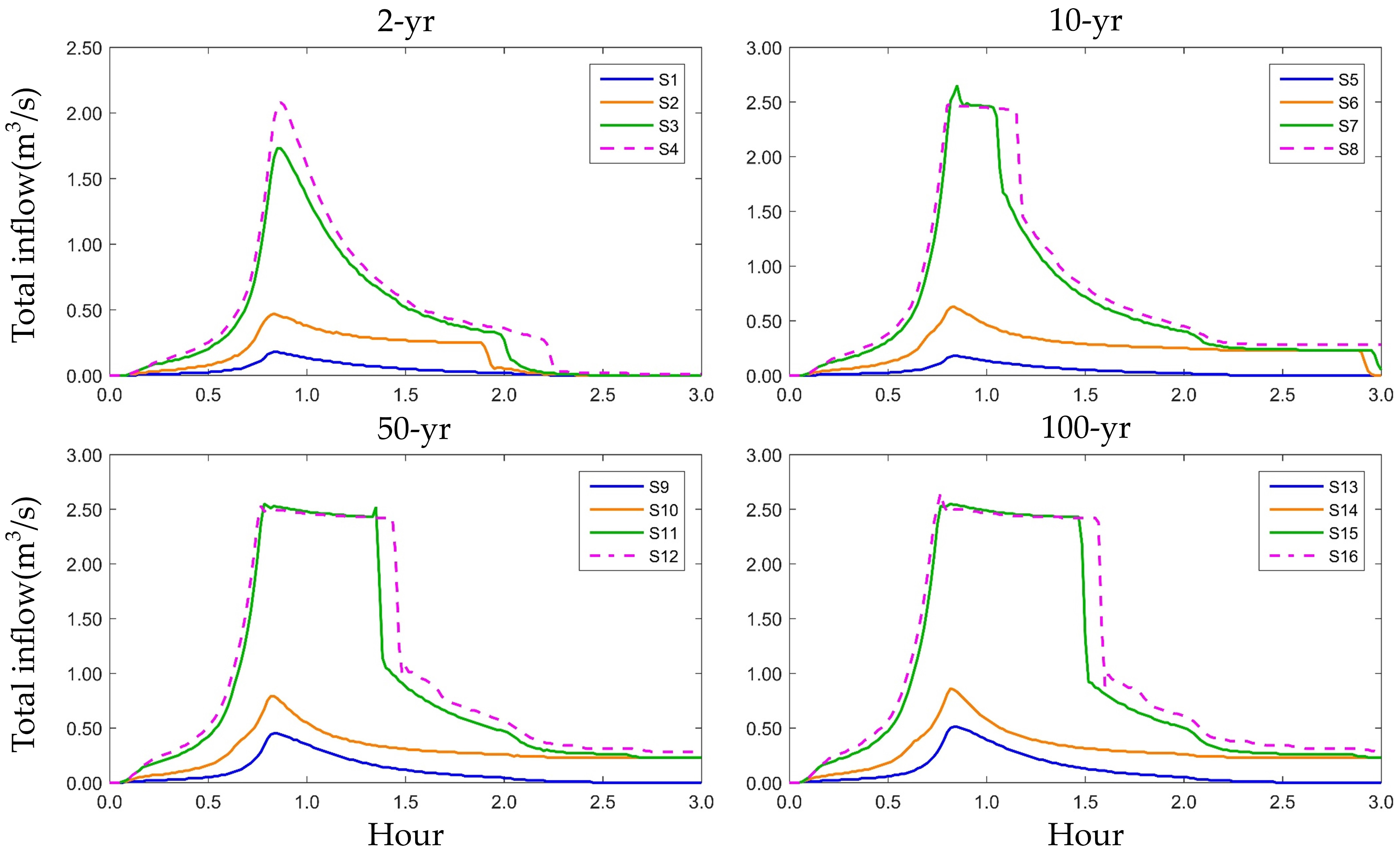
Figure 11, Figure 12 and Figure 13 show the time–total inflow hydrographs of S1–S16 for the 1Y108 outfall in the northern district, for the 4Y455 outfall in the convention district, and for the 3Y80 outfall in the main district, respectively.
For the time–total inflow hydrographs of outfall 1Y108 in the northern district (Figure 11), the hydrographs results of Levels 1–3 were very close to those Level 4 and each other for the 2-year storm. Similarly, for the 10-, 50-, and 100-year storms, the time–total inflow hydrographs of the experimental group were very close to the control group, although the Level 1 hydrographs tended to deviate from the Level 4 hydrographs (i.e., control groups) as the heavy rainfall increased. However, the differences between Levels 1 and 4 were not great.
For the time–total inflow hydrographs of outfall 4Y455 in the convention district (Figure 12), note that the difference between hydrographs for the same storm were clearer than the hydrographs of the northern district. In addition, the Level 1 and Level 2 hydrographs were very close to each other for each storm, while the Level 3 and Level 4 hydrographs were very close to each other. The difference between Levels 3 and 4 increased with rainfall but only marginally. The differences between Levels 1 or 2 and Level 4 showed a subtle increasing trend.
The time–total inflow hydrographs of outfall 3Y80 in the main district were the most distinct for the four levels of all outfalls (Figure 13). Surprisingly, the differences between hydrographs for the same storm were significant compared with the hydrographs of the northern and convention districts. Overall, the Level 3 hydrographs were very close to the Level 4 hydrographs, but the Level 1 and Level 2 hydrographs were far from the Level 4 hydrographs. This means that the simulation results will be unreliable if a Level 1 or 2 generalization is adopted but will be acceptable with a Level 3 generalization.
Notably, the difference of four levels’ time–total inflow hydrographs of the three districts which had different amounts of outfall clearly show a different situation. This is because, if a certain area has more than one drainage system, simplification of the drainage system may lead to erroneous division of the subcatchments. This can result in storm runoff that should originally flow into one drainage system being assigned to another drainage system.
Therefore, when the study area had only one drainage system, the time–total inflow hydrograph was almost unaffected by the generalization degree of the sewer network. However, when the study area had more than one drainage system, the time–total inflow hydrograph could deviate from the actual results depending on the generalization degree of the sewer network leading to the erroneous division of subcatchments. A higher degree of simplification of the sewer network would clearly increase the probability of erroneous division of subcatchments for an area with multiple drainage systems. Thus, the solution is to extend the range of the generalized sewer network to be as similar as possible to the original network to minimize the error (e.g., Level 3 in the main district).
4.3. Flood Results
We analyzed the distribution of overflow points, total overflow, flood spreading area, and accumulated flood depth to further explore the impact of the generalization degree of the sewer network on the flood simulation results. The accumulated flood depth was calculated by using the total overflow of the overflow points divided by the area of the corresponding subcatchments.
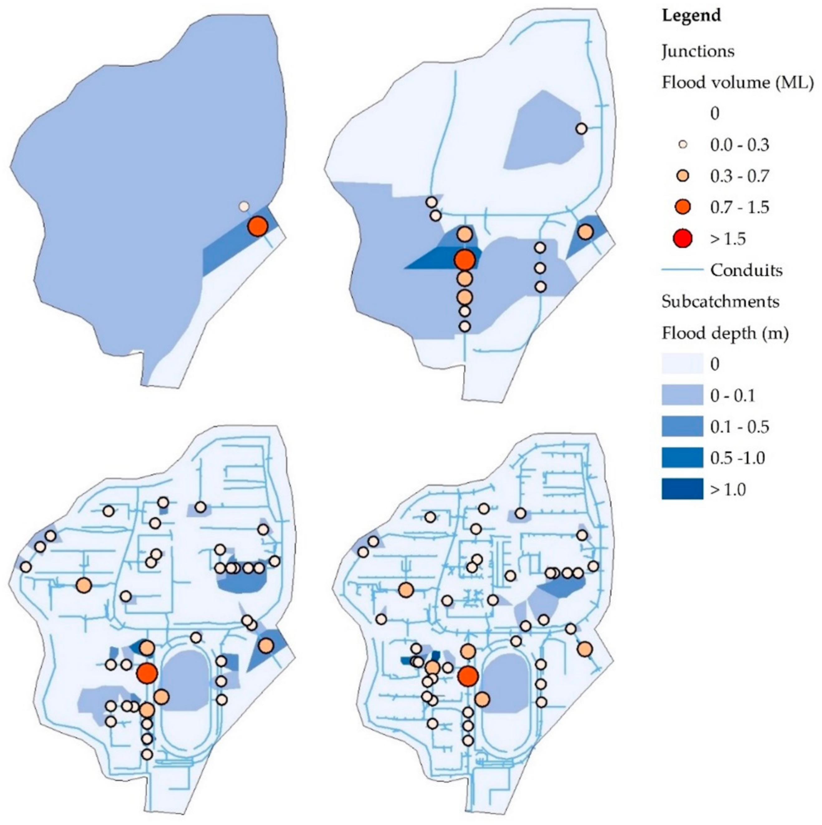
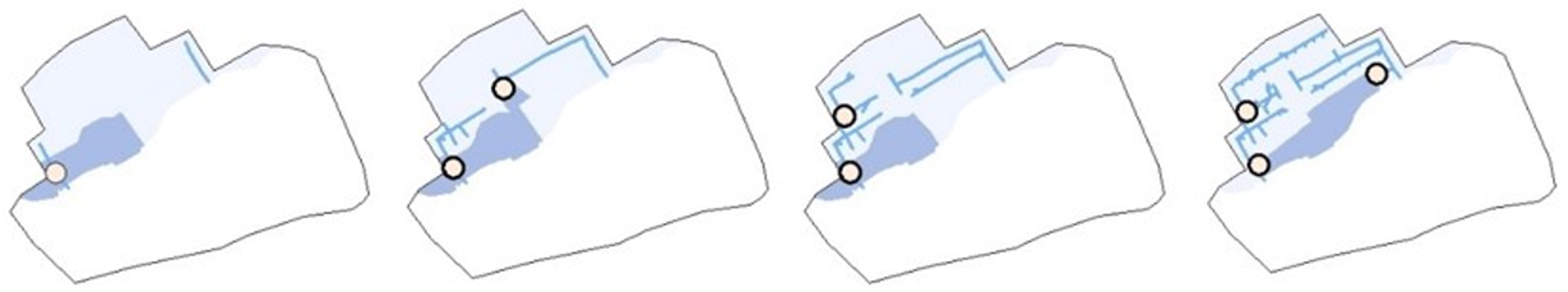
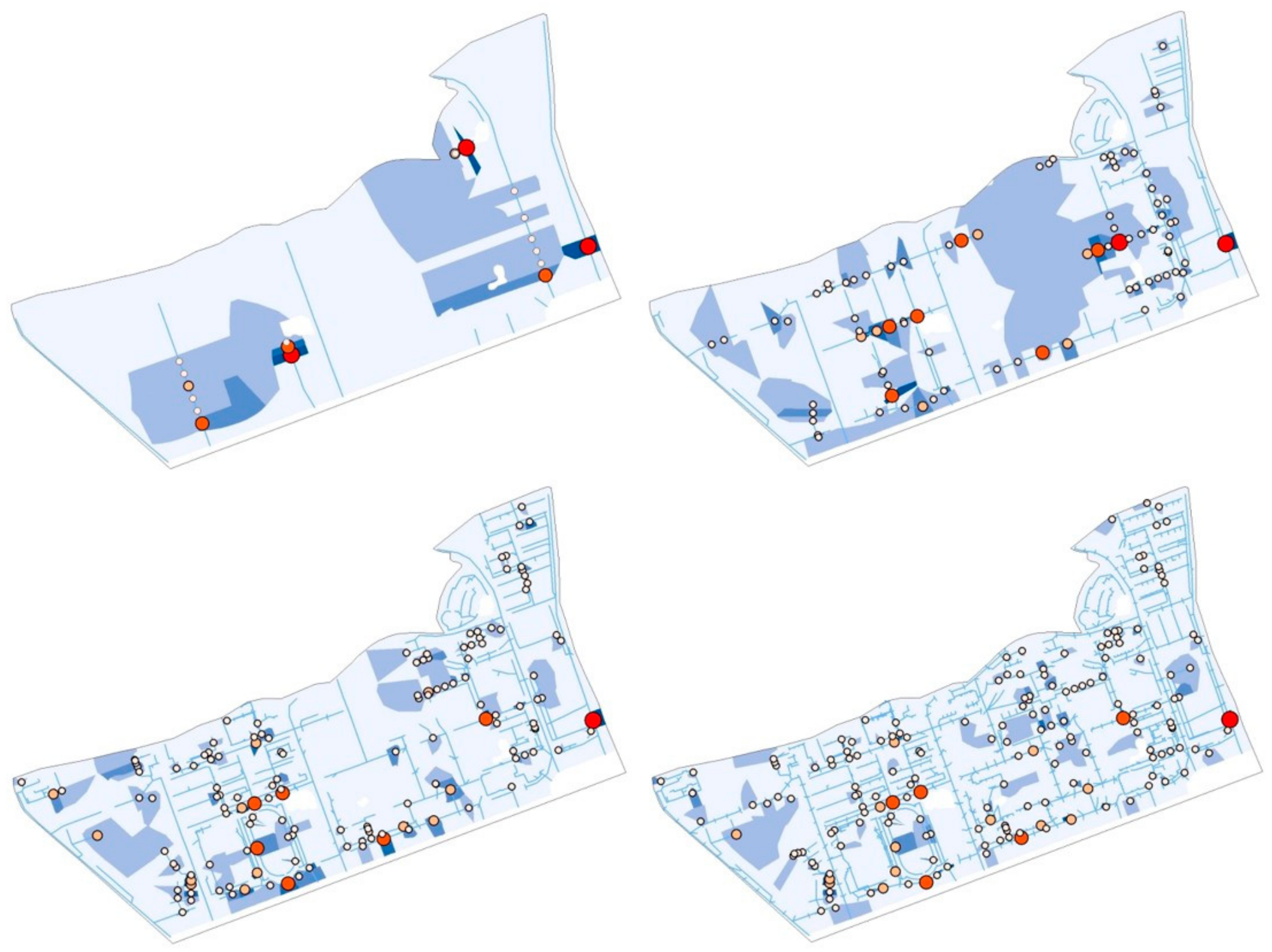
We only analyzed the flood simulation results for the storm with a 50-year return period (Scenarios S9–S12) because the simulation results were similar for other return periods. Figure 14, Figure 15 and Figure 16 show the distribution of overflow points and accumulated flood depth of Scenarios S9–S12 for the three sub-basins. The statistical results are presented in Table 5 for the northern district, Table 6 for the convention district, and Table 7 for the main district. N is the number of overflow points, TN is the total number of overflow points, SLN is the same number of overflow point locations compared with S12 with a Level 4 network complexity (i.e., control group), A is the inundated area, and TA is the total inundated area.
The simulation results showed that the number of overflow points increased with the complexity of the sewer network in the northern district (see Figure 14 and Table 5). The other districts showed a similar trend, as presented in Figure 15 and Figure 16 and Table 6 and Table 7. This means that increasing the degree of generalization of the sewer network reduces the accuracy regarding the location of overflow points.
However, Figure 14, Figure 15 and Figure 16 show that overflow points with serious flooding (i.e., flood volume of greater than 0.3 ML) were mainly distributed on the backbone conduits. When the flood volume of overflow points was 0.31–0.70 ML, N and SLM of Level 1 and Level 2 were quite different from the values of Level 4, but the values of Level 3 were very close to those of Level 4. When the flood volume of the overflow points was 0.71–1.50 ML or ≥1.51 ML, the differences in values between the experimental and control groups were reduced. The results showed that a simplified sewer network that keeps the backbone conduits of the drainage system can identify serious overflow points to some extent. In other words, the simplified sewer network can catch similar serious overflow points provided that it extends over a similar region as the original sewer network.
The total inundated area (TA) in the northern district decreased with increasing complexity for S9–S12, as presented in Table 5. The same situation was observed in the main district, as presented in Table 7. This indicates that increasing the degree of generalization of the sewer network makes it more difficult to obtain specific locations of the inundated area, and only a rough range can be obtained.
In general, the total overflow, flood spreading area, and accumulated flood depth of Level 3 were quite close to those of Level 4. Thus, we can use a Level 3 generalization to simulate floods in the study area instead of Level 4. However, if we do not require high precision in the simulation and only need to identify areas with serious overflow, Level 2 can be considered to replace Level 4, but Level 1 is inappropriate owing to critical error.
5. Conclusions
In this study, we designed 16 scenarios for three sub-basins based on four different complexities for sewer networks and four storms with different return periods to explore the impact of the urban drainage system complexity on the flood simulation accuracy in terms of the total inflow of outfall and flood results. We also proposed the stroke scaling method for automatic generalization to overcome the low efficiency and accuracy of manual generalization.
The results of the three specific case studies showed that the complexity of the urban storm sewer network does not have a significant impact on the total inflow of outfalls for a single drainage system but does have a clear impact for multiple drainage systems. The driving factor is that simplifying a region with multiple drainage systems may induce the storm runoff to flow into the wrong drainage systems. The results also showed that serious flooding is mainly distributed on backbone pipes. This means that, if the simplified sewer network extends over a range similar to that of the original network, the flood simulation results for the two networks will be similar. The results of the research basins can be used to formulate the following generalization strategies for a storm sewer network.
(1) Extreme rainfall intensity does not need to be considered for storm sewer network generalization because the differences in the flood simulation results for different complexities of the sewer network with different storm intensities are not quite clear.
(2) If the whole area for flood simulation is large and there are no strict requirement for the accuracy of inundated locations in the small sub-basins, sub-basins with a single drainage system can be considerably simplified to only keep conduits and junctions that are directly connected with the outfall (i.e., keep pipe strokes with Le = 1). Sub-basins with multiple drainage systems should also keep the conduits and junctions that make up the backbone of the original sewer network. However, if there are strict requirements regarding the quality of the flood simulation results, the conduits and junctions making up the backbone of the original sewer network should also be kept for sub-basins with a single drainage system.
(3) If the flood simulation area is small and locations with serious inundation need to be located, the simplified sewer network should be extended to have a range similar to that of the original sewer network. Therefore, the generalization strategy should be removing the branch sections of the sewer network first rather than deleting upstream segments without considering the range of the drainage system.
In summary, the storm sewer network should be simplified depending on the distribution characteristics of the drainage system and required precision for the flood simulation results. We believe that this study is greatly significant regarding data precision for the sensitivity of flood simulation. In addition, the proposed generalization strategies and automatic generalization method of storm sewer networks are highly applicable to improving the quality and efficiency of flood modeling and simulation.
However, this study focused only on the accuracy of storm sewer network on the sensitivity of flood simulations in an urban area. Future studies will explore the precision of other datasets and its effect on the sensitivity of hydrologic modeling or simulation in different scenarios. Different data precisions of different datasets can be compared to discover laws or patterns for the model sensitivity. Then, a series of simplified strategies can be proposed for different data types or combinations of different datasets to improve modeling and simulation efficiency.
Author Contributions
Q.Y. was responsible for the literature search, setting up the experiments, completing most of the experiments, and writing the initial draft of the manuscript. Q.D., D.H., and S.Z. principally conceived the idea and design of the study and provided financial support. X.Z. was responsible for the figures.
Acknowledgments
This study was supported by Newton Fund via Natural Environment Research Council (NERC) and Economic and Social Research Council (ESRC) (NE/N012143/1), and the National Natural Science Foundation of China (Nos.: 41771424, 41501429), and the Top-notch Academic Programs Project of Jiangsu Higher Education Institutions (TAPP), and the University Natural Science Project of Jiangsu Province (Grant No. 16KJA170001).
Conflicts of Interest
The authors declare no conflict of interest.
References
- Chen, Y.; Zhou, H.; Zhang, H.; Du, G.; Zhou, J. Urban flood risk warning under rapid urbanization. Environ. Res. 2015, 139, 3–10. [Google Scholar] [CrossRef] [PubMed]
- Hammond, M.J.; Chen, A.S.; Djordjević, S.; Butler, D.; Mark, O. Urban flood impact assessment: A state-of-the-art review. Urban Water J. 2015, 12, 14–29. [Google Scholar] [CrossRef]
- Zevenbergen, C.; Pathirana, A. Managing urban flooding in the face of continuous change. In Resilience and Urban Risk Management; Taylor & Francis Group: London, UK, 2012; pp. 73–77. [Google Scholar]
- Mendes, J.; Maia, R. Hydrologic modelling calibration for operational flood forecasting. Water Resour. Manag. 2016, 30, 5671–5685. [Google Scholar] [CrossRef]
- Nanía, L.S.; León, A.S.; García, M.H. Hydrologic-hydraulic model for simulating dual drainage and flooding in urban areas: Application to a catchment in the metropolitan area of chicago. J. Hydrol. Eng. 2014, 20, 04014071. [Google Scholar] [CrossRef]
- Zappa, M.; Jaun, S.; Germann, U.; Walser, A.; Fundel, F. Superposition of three sources of uncertainties in operational flood forecasting chains. Atmos. Res. 2011, 100, 246–262. [Google Scholar] [CrossRef]
- Hutchins, M.G.; McGrane, S.J.; Miller, J.D.; Hagen-Zanker, A.; Kjeldsen, T.R.; Dadson, S.J.; Rowland, C.S. Integrated modeling in urban hydrology: Reviewing the role of monitoring technology in overcoming the issue of ‘big data’ requirements. Wiley Interdiscip. Rev. Water 2017, 4. [Google Scholar] [CrossRef]
- Kang, R.S.; Marston, R.A. Geomorphic effects of rural-to-urban land use conversion on three streams in the central redbed plains of oklahoma. Geomorphology 2006, 79, 488–506. [Google Scholar] [CrossRef]
- Yu, D.; Coulthard, T.J. Evaluating the importance of catchment hydrological parameters for urban surface water flood modelling using a simple hydro-inundation model. J. Hydrol. 2015, 524, 385–400. [Google Scholar] [CrossRef] [Green Version]
- Czubski, K.; Kozak, J.; Kolecka, N. Accuracy of SRTM-x and ASTER elevation data and its influence on topographical and hydrological modeling: Case study of the pieniny Mts. in Poland. Int. J. Geoinform. 2013, 9. [Google Scholar] [CrossRef]
- Dai, Q.; Han, D.; Zhuo, L.; Huang, J.; Islam, T.; Srivastava, P.K. Impact of complexity of radar rainfall uncertainty model on flow simulation. Atmos. Res. 2015, 161–162, 93–101. [Google Scholar] [CrossRef]
- Hunter, N.; Bates, P.; Neelz, S.; Pender, G.; Villanueva, I.; Wright, N.; Liang, D.; Falconer, R.A.; Lin, B.; Waller, S. Benchmarking 2D hydraulic models for urban flood simulations. In Proceedings of the Institution of Civil Engineers: Water Management; Thomas Telford (ICE Publishing): London, UK, 2008; pp. 13–30. [Google Scholar]
- Wałęga, A.; Książek, L. The effect of a hydrological model structure and rainfall data on the accuracy of flood description in an upland catchment. Ann. Wars. Univ. Life Sci. Land Reclam. 2015, 47, 305–320. [Google Scholar] [CrossRef]
- Croci, S.; Paoletti, A.; Tabellini, P. Urbfep model for basin scale simulation of urban floods constrained by sewerage’s size limitations. Procedia Eng. 2014, 70, 389–398. [Google Scholar] [CrossRef]
- Hsu, M.H.; Chen, S.H.; Chang, T.J. Inundation simulation for urban drainage basin with storm sewer system. J. Hydrol. 2000, 234, 21–37. [Google Scholar] [CrossRef] [Green Version]
- Sharifan, R.A.; Roshan, A.; Aflatoni, M.; Jahedi, A.; Zolghadr, M. Uncertainty and sensitivity analysis of SWMM model in computation of manhole water depth and subcatchment peak flood. Procedia Soc. Behav. Sci. 2010, 2, 7739–7740. [Google Scholar] [CrossRef]
- Cleveland, T.G.; Luong, T.; Thompson, D.B. Water Subdivision for Modeling. In World Environmental and Water Resources Congress 2009: Great Rivers; American Society of Civil Engineers: Reston, VA, USA, 2009; pp. 1–10. [Google Scholar]
- Elliott, A.H.; Trowsdale, S.A.; Wadhwa, S. Effect of aggregation of on-site storm-water control devices in an urban catchment model. J. Hydrol. Eng. 2009, 14, 975–983. [Google Scholar] [CrossRef]
- Zhang, W.; Montgomery, D.R. Digital elevation model grid size, landscape representation, and hydrologic simulations. Water Resour. Res. 1994, 30, 1019–1028. [Google Scholar] [CrossRef]
- Chaplot, V. Impact of dem mesh size and soil map scale on swat runoff, sediment, and no3–n loads predictions. J. Hydrol. 2005, 312, 207–222. [Google Scholar] [CrossRef]
- Chaubey, I.; Cotter, A.; Costello, T.; Soerens, T. Effect of dem data resolution on swat output uncertainty. Hydrol. Process. 2005, 19, 621–628. [Google Scholar] [CrossRef]
- Yu, D.; Lane, S.N. Urban fluvial flood modelling using a two-dimensional diffusion-wave treatment, part 1: Mesh resolution effects. Hydrol. Process. 2006, 20, 1541–1565. [Google Scholar] [CrossRef]
- Yu, D.; Lane, S.N. Urban fluvial flood modelling using a two-dimensional diffusion-wave treatment, part 2: Development of a sub-grid-scale treatment. Hydrol. Process. 2006, 20, 1567–1583. [Google Scholar] [CrossRef]
- Tripathi, M.; Raghuwanshi, N.; Rao, G. Effect of watershed subdivision on simulation of water balance components. Hydrol. Process. 2006, 20, 1137–1156. [Google Scholar] [CrossRef]
- Carpenter, T.M.; Georgakakos, K.P. Impacts of parametric and radar rainfall uncertainty on the ensemble streamflow simulations of a distributed hydrologic model. J. Hydrol. 2004, 298, 202–221. [Google Scholar] [CrossRef]
- Ghosh, I.; Hellweger, F.L. Effects of spatial resolution in urban hydrologic simulations. J. Hydrol. Eng. 2011, 17, 129–137. [Google Scholar] [CrossRef]
- Krebs, G.; Kokkonen, T.; Valtanen, M.; Setälä, H.; Koivusalo, H. Spatial resolution considerations for urban hydrological modelling. J. Hydrol. 2014, 512, 482–497. [Google Scholar] [CrossRef]
- Park, S.Y.; Lee, K.W.; Park, I.H.; Ha, S.R. Effect of the aggregation level of surface runoff fields and sewer network for a swmm simulation. Desalination 2008, 226, 328–337. [Google Scholar] [CrossRef]
- Rossman, L.A. Storm Water Management Model User’s Manual, Version 5.0; National Risk Management Research Laboratory, Office of Research and Development, US Environmental Protection Agency Cincinnati: Cincinnati, OH, USA, 2010.
- Peterson, E.W.; Wicks, C.M. Assessing the importance of conduit geometry and physical parameters in karst systems using the storm water management model (SWMM). J. Hydrol. 2006, 329, 294–305. [Google Scholar] [CrossRef]
- Cambez, M.; Pinho, J.; David, L. Using SWMM 5 in the continuous modelling of stormwater hydraulics and quality. In Proceedings of the 11th International Conference on Urban Drainage, Edinburgh, Scotland, UK, 31 August–5 September 2008. [Google Scholar]
- Yu, P.-S.; Yang, T.-C.; Chen, S.-J. Comparison of uncertainty analysis methods for a distributed rainfall–runoff model. J. Hydrol. 2001, 244, 43–59. [Google Scholar] [CrossRef]
- Choi, K.-S.; Ball, J.E. Parameter estimation for urban runoff modelling. Urban Water 2002, 4, 31–41. [Google Scholar] [CrossRef]
- Shen, J.; Zhang, Q. Parameter estimation method for swmm under the condition of incomplete information based on GIS and RS. Electron. J. Geotech. Eng. 2014, 20, 6095–6108. [Google Scholar]
- Zhao, D.; Chen, J.; Wang, H.; Tong, Q.; Cao, S.; Sheng, Z. GIS-based urban rainfall-runoff modeling using an automatic catchment-discretization approach: A case study in macau. Environ. Earth Sci. 2009, 59, 465. [Google Scholar] [CrossRef]
- Eslamian, S. Handbook of Engineering Hydrology: Modeling, Climate Change, and Variability; CRC Press: Boca Raton, FL, USA, 2014. [Google Scholar]
- Lhomme, J.; Bouvier, C.; Perrin, J.-L. Applying a GIS-based geomorphological routing model in urban catchments. J. Hydrol. 2004, 299, 203–216. [Google Scholar] [CrossRef]
- Akhter, M.S.; Hewa, G.A. The use of PCSWMM for assessing the impacts of land use changes on hydrological responses and performance of WSUD in managing the impacts at myponga catchment, South Australia. Water 2016, 8, 511. [Google Scholar] [CrossRef]
- Mancipe-Munoz, N.A.; Buchberger, S.G.; Suidan, M.T.; Lu, T. Calibration of rainfall-runoff model in urban watersheds for stormwater management assessment. J. Water Resour. Plan. Manag. 2014, 140, 05014001. [Google Scholar] [CrossRef]
- Li, Z.; Dong, W. A stroke-based method for automated generation of schematic network maps. Int. J. Geogr. Inf. Sci. 2010, 24, 1631–1647. [Google Scholar] [CrossRef]
- Porta, S.; Crucitti, P.; Latora, V. The network analysis of urban streets: A primal approach. Environ. Plan. B Plan. Des. 2006, 33, 705–725. [Google Scholar] [CrossRef]
- Thomson, R.C.; Richardson, D.E. The ‘good continuation’principle of perceptual organization applied to the generalization of road networks. In Proceedings Actes; Ottawa ICA 1999: Ottawa, ON, Canada, 1999. [Google Scholar]
- Madsen, H.; Mikkelsen, P.S.; Rosbjerg, D.; Harremoës, P. Regional estimation of rainfall intensity-duration-frequency curves using generalized least squares regression of partial duration series statistics. Water Resour. Res. 2002, 38. [Google Scholar] [CrossRef]
- Willems, P.; Arnbjerg-Nielsen, K.; Olsson, J.; Nguyen, V.T.V. Climate change impact assessment on urban rainfall extremes and urban drainage: Methods and shortcomings. Atmos. Res. 2012, 103, 106–118. [Google Scholar] [CrossRef]
- Che, G.; Shen, J.; Fan, R. Research on rainfall pattern of urban design storm. Adv. Water Sci. 1998, 9, 41–46. [Google Scholar]
- Zhu, J.; Dai, Q.; Deng, Y.; Zhang, A.; Zhang, Y.; Zhang, S. Indirect damage of urban flooding: Investigation of flood-induced traffic congestion using dynamic modeling. Water 2018, 10, 622. [Google Scholar] [CrossRef]
Figure 1.
Catchment discretization based on geographic information system (GIS) techniques.

Figure 2.
Algorithm program flowchart for pipe strokes construction.

Figure 3.
Algorithm program flowchart for each pipe stroke construction.

Figure 4.
Example of pipe stroke construction. The plot on the left side of the arrow is the original sewer network, and the right side shows the corresponding pipe strokes.
Figure 4.
Example of pipe stroke construction. The plot on the left side of the arrow is the original sewer network, and the right side shows the corresponding pipe strokes.

Figure 5.
Classification results for the example storm sewer network in Figure 4.
Figure 5.
Classification results for the example storm sewer network in Figure 4.

Figure 6.
Location of the study area, which contains three separated sub-basins: the northern district, convention district, and main district.
Figure 6.
Location of the study area, which contains three separated sub-basins: the northern district, convention district, and main district.

Figure 7.
Distribution of the storm sewer networks in the three sub-basins. The red triangles represent outfalls, which are terminal nodes of the drainage system. The blue dots represent junctions where links join together. The light blue line represents conduits that move water from one node to another.

Figure 8.
Classification results for four levels of the sewer network and the corresponding discretization results for the northern district.
Figure 8.
Classification results for four levels of the sewer network and the corresponding discretization results for the northern district.

Figure 9.
Classification results for four levels of the sewer network and the corresponding discretization results for the convention district.
Figure 9.
Classification results for four levels of the sewer network and the corresponding discretization results for the convention district.

Figure 10.
Classification results for four levels of the sewer network and the corresponding discretization results for the main district.
Figure 10.
Classification results for four levels of the sewer network and the corresponding discretization results for the main district.

Figure 11.
Total inflow hydrographs of outfall 1Y108 in the northern district for the 16 scenarios.

Figure 12.
Total inflow hydrographs of outfall 4Y455 in the convention district for the 16 scenarios.
Figure 12.
Total inflow hydrographs of outfall 4Y455 in the convention district for the 16 scenarios.

Figure 13.
Total inflow hydrographs of outfall 3Y80 in the main district for the 16 scenarios.

Figure 14.
Distribution of the overflow junctions and flood area, flood volume of the overflow junctions, and flood depth of the flood subcatchments for the northern district. In the legend, “ML” represents a million liters, and “m” represents meters.
Figure 14.
Distribution of the overflow junctions and flood area, flood volume of the overflow junctions, and flood depth of the flood subcatchments for the northern district. In the legend, “ML” represents a million liters, and “m” represents meters.

Figure 15.
Distribution of the overflow junctions and flood area, flood volume of the overflow junctions, and flood depth of the flood subcatchments for the convention district.
Figure 15.
Distribution of the overflow junctions and flood area, flood volume of the overflow junctions, and flood depth of the flood subcatchments for the convention district.

Figure 16.
Distribution of overflow junctions and flood area, flood volume of the overflow junctions, and flood depth of the flood subcatchments for the main district.
Figure 16.
Distribution of overflow junctions and flood area, flood volume of the overflow junctions, and flood depth of the flood subcatchments for the main district.


Table 1.
Properties of the drainage system for the three sub-basins.
| Northern Distract | Convention District | Main Distract | |
|---|---|---|---|
| Area (ha) | 15.83 | 3.47 | 60.00 |
| Impermeability (%) | 70.84 | 28.56 | 64.62 |
| Total length (km) | 9.15 | 0.60 | 26.22 |
| Number of junctions | 1057 | 97 | 2701 |
| Number of outfalls | 1 | 2 | 11 |
Table 2.
Scenario design in this study.
| Scenarios | Complexity | Subdivisions | Storms |
|---|---|---|---|
| S1 | Level 1 | Subdivision 1 | 2-year |
| S2 | Level 2 | Subdivision 2 | 2-year |
| S3 | Level 3 | Subdivision 3 | 2-year |
| S4 | Level 4 | Subdivision 4 | 2-year |
| S5 | Level 1 | Subdivision 1 | 10-year |
| S6 | Level 2 | Subdivision 2 | 10-year |
| S7 | Level 3 | Subdivision 3 | 10-year |
| S8 | Level 4 | Subdivision 4 | 10-year |
| S9 | Level 1 | Subdivision 1 | 50-year |
| S10 | Level 2 | Subdivision 2 | 50-year |
| S11 | Level 3 | Subdivision 3 | 50-year |
| S12 | Level 4 | Subdivision 4 | 50-year |
| S13 | Level 1 | Subdivision 1 | 100-year |
| S14 | Level 2 | Subdivision 2 | 100-year |
| S15 | Level 3 | Subdivision 3 | 100-year |
| S16 | Level 4 | Subdivision 4 | 100-year |
Table 3.
Conduit length and subcatchment counts for different drainage system complexities of the three sub-basins.
Table 3.
Conduit length and subcatchment counts for different drainage system complexities of the three sub-basins.
| Sub-Basins | Statistics | Level 1 | Level 2 | Level 3 | Level 4 |
|---|---|---|---|---|---|
| Northern district | Conduits length (km) | 0.08 | 1.54 | 6.58 | 9.15 |
| Subcatchments counts | 3 | 79 | 531 | 1055 | |
| Convention district | Conduits length | 0.07 | 0.23 | 0.43 | 0.60 |
| Subcatchments counts | 5 | 22 | 47 | 96 | |
| Main district | Conduits length | 2.90 | 9.80 | 18.70 | 27.00 |
| Subcatchments counts | 114 | 519 | 1336 | 2717 |
Table 4.
Cost time of simulating four levels of sewer networks for a storm with a 50-year return period.
Table 4.
Cost time of simulating four levels of sewer networks for a storm with a 50-year return period.
| Sub-Basins | Level 1 (s) | Level 2 | Level 3 | Level 4 |
|---|---|---|---|---|
| Northern district | 0.01 | 0.11 | 0.79 | 1.57 |
| Convention district | 0.01 | 0.03 | 0.08 | 0.14 |
| Main district | 0.14 | 0.70 | 1.85 | 4.09 |
Table 5.
The total number of overflow points (TN), the number of overflow points (N), the same number of overflow point locations compared with the control group (SLM), and the total inundated area (TA) of Scenarios S9–S12 for the northern district.
Table 5.
The total number of overflow points (TN), the number of overflow points (N), the same number of overflow point locations compared with the control group (SLM), and the total inundated area (TA) of Scenarios S9–S12 for the northern district.
| Scenarios | TN | 0.00–0.30 ML | 0.31–0.70 ML | 0.71–1.50 ML | ≥1.51 ML | TA (ha) | ||||
|---|---|---|---|---|---|---|---|---|---|---|
| N | SLM | N | SLM | N | SLM | N | SLM | |||
| S9 | 2 | 1 | 0 | 0 | 0 | 1 | 0 | 0 | 0 | 14.76 |
| S10 | 13 | 8 | 5 | 4 | 2 | 1 | 1 | 0 | 0 | 5.70 |
| S11 | 39 | 33 | 24 | 5 | 4 | 1 | 1 | 0 | 0 | 2.27 |
| S12 | 433 | 37 | 37 | 5 | 5 | 1 | 1 | 0 | 0 | 1.67 |
Table 6.
TN, N, SLM, and TA of Scenarios S9–S12 for the convention district.
| Scenarios | TN | 0.00–0.30 ML | 0.31–0.70 ML | 0.71–1.50 ML | ≥1.51 ML | TA (ha) | ||||
|---|---|---|---|---|---|---|---|---|---|---|
| N | SLM | N | SLM | N | SLM | N | SLM | |||
| S9 | 1 | 1 | 0 | 0 | 0 | 0 | 0 | 0 | 0 | 0.24 |
| S10 | 2 | 2 | 0 | 0 | 0 | 0 | 0 | 0 | 0 | 0.25 |
| S11 | 2 | 2 | 1 | 0 | 0 | 0 | 0 | 0 | 0 | 0.23 |
| S12 | 3 | 3 | 3 | 0 | 0 | 0 | 0 | 0 | 0 | 0.25 |
Table 7.
TN, N, SLM, and TA of Scenarios S9–S12 for the main district.
| Scenarios | TN | 0.00–0.30 ML | 0.31–0.70 ML | 0.71–1.50 ML | ≥1.51 ML | TA (ha) | ||||
|---|---|---|---|---|---|---|---|---|---|---|
| N | SLM | N | SLM | N | SLM | N | SLM | |||
| S9 | 19 | 11 | 0 | 2 | 0 | 3 | 0 | 3 | 1 | 16.74 |
| S10 | 85 | 71 | 36 | 6 | 2 | 6 | 2 | 2 | 1 | 19.68 |
| S11 | 143 | 124 | 98 | 12 | 10 | 6 | 5 | 1 | 1 | 10.03 |
| S12 | 179 | 160 | 160 | 13 | 13 | 5 | 5 | 1 | 1 | 7.82 |
© 2018 by the authors. Licensee MDPI, Basel, Switzerland. This article is an open access article distributed under the terms and conditions of the Creative Commons Attribution (CC BY) license (http://creativecommons.org/licenses/by/4.0/).
Share and Cite
MDPI and ACS Style
Yang, Q.; Dai, Q.; Han, D.; Zhu, X.; Zhang, S. Impact of the Storm Sewer Network Complexity on Flood Simulations According to the Stroke Scaling Method. Water 2018, 10, 645. https://doi.org/10.3390/w10050645
AMA Style
Yang Q, Dai Q, Han D, Zhu X, Zhang S. Impact of the Storm Sewer Network Complexity on Flood Simulations According to the Stroke Scaling Method. Water. 2018; 10(5):645. https://doi.org/10.3390/w10050645
Chicago/Turabian StyleYang, Qiqi, Qiang Dai, Dawei Han, Xuehong Zhu, and Shuliang Zhang. 2018. "Impact of the Storm Sewer Network Complexity on Flood Simulations According to the Stroke Scaling Method" Water 10, no. 5: 645. https://doi.org/10.3390/w10050645
Note that from the first issue of 2016, this journal uses article numbers instead of page numbers. See further details here.