TWI Computations and Topographic Analysis of Depression-Dominated Surfaces


Department of Civil and Environmental Engineering (Dept 2470), North Dakota State University, P.O. Box 6050, Fargo, ND 58108-6050, USA
*
Author to whom correspondence should be addressed.
Water 2018, 10(5), 663; https://doi.org/10.3390/w10050663
Submission received: 25 March 2018
/
Revised: 21 April 2018
/
Accepted: 17 May 2018
/
Published: 19 May 2018
(This article belongs to the Section Hydrology)
Abstract
:The topographic wetness index (TWI) has been widely used for determining the potential of each digital elevation model (DEM) grid to develop a saturated condition, which allows for the investigation of topographic control on the hydrologic response of a watershed. Many studies have evaluated TWI, its components, and the impacts of DEM resolution on its computation. However, the majority of the studies are concerned with typical dendritic watersheds, and the effectiveness of TWI computations for depression-dominated areas has been rarely evaluated. The objectives of this study are (1) to develop a modified TWI computation procedure for depression-dominated areas, (2) to examine the differences between the new and existing TWI computation procedures using different DEMs, and (3) to assess the impact of DEM resolution on the new TWI procedure. In particular, a bathymetry survey was conducted for a study area in the Prairie Pothole Region (PPR), and the DEM representing the actual surface topography was created. The statistical analyses of TWI highlighted a two-hump pattern for the depression-dominated surface, whereas a one-hump pattern was observed for the dendritic surface. It was observed that depressional DEM grids accounted for higher values of TWI than other grids. It was demonstrated that a filled DEM led to misleading quantity and distribution of TWI for depression-dominated landscapes. The modified TWI computation procedure proposed in this study can also be applied to other depression-dominated areas.
1. Introduction
Topographic wetness index (TWI) determines the topographic control on the hydrologic response of a watershed [1,2]. Initially, Beven and Kirkby [1] developed a computerized procedure to calculate TWI based on gridded DEMs. Gridded DEMs are used to perform topographic analysis and investigate land surface processes from different aspects such as biodiversity and wetlands studies (e.g., [3,4]). TWI is calculated for each DEM grid on a surface as , in which is the upslope contributing area per unit length of contour and represents the slope of the water table [1]. In practice, is usually estimated as the land surface gradient that can be calculated from gridded DEMs. Grids with higher TWI are associated with higher likelihood of saturation. This index provides a foundation to predict variable source areas (VSAs) (i.e., runoff-generating areas with varying size and location over time [5,6]. Also, TWI allows hydrologic models to take advantage of topographic analysis [7,8,9,10]. Since computation of TWI is directly associated with gridded DEMs, many studies over the course of the last two decades have addressed the impacts of DEM resolution on TWI [11,12,13,14,15]. For example, Saulnier et al. [12] showed that the mean of TWI increased for coarser resolutions. Vaze et al. [13] suggested utilizing high-resolution DEMs, instead of coarser ones. Sørensen and Seibert [14] investigated the information content of DEMs and concluded that a finer resolution was not necessarily the optimal one.
A gridded DEM may include numerous depressions. Some depressions are created as a result of errors in the measurement or interpolation procedure (i.e., artifacts). These depressions can be referred to as spurious pits/sinks [16,17]. On the other hand, the other types of depressions are de facto (micro)topographic features of land surfaces and play an important role in surface and subsurface hydrologic processes [3,18,19,20,21,22]. The Prairie Pothole Region (PPR) located in the US and Canada is an example of areas with de facto depressions that have significant influences on hydrologic processes [22]. Depressions act like “gate keepers” in depression-dominated areas [22,23]. They delay the surface runoff generation process by storing overland flow and releasing water through their thresholds when they are fully filled. Since the presence of depressions is considered to be a barrier for hydrologic modeling [3,22], most existing delineation methods are based on depressionless DEMs [24,25,26,27,28]. In other words, different delineation methods fill/remove all depressions (including de facto and spurious depressions) and specify artificial flow direction and flow accumulation values [19] to ensure that the surface is hydrologically connected [29,30]. In addition, available DEMs of landscapes only provide a snapshot of one past representation of surface elevations, instead of the actual land surface elevations for a modeling time period.
Several studies have addressed these shortcomings from different aspects [18,21,31]. For example, Chu et al. [31] introduced a Puddle-Delineation (PD) algorithm that takes advantage of DEMs and provides elaborate microtopographic characteristics such as depression storage, ponding area, the hierarchical relationship between puddles, mean depth of puddles, and other topographic parameters. PD provides fundamental topographic data for the Puddle-to-Puddle (P2P) modeling system [18]. By incorporating the PD results, the P2P system simulates the dynamic P2P filling, spilling, merging, and splitting processes for depression-dominated areas [18]. Further, Tahmasebi Nasab [23] introduced the Depression-Dominated Delineation (D-cubed) method in which each sub-basin is divided into a number of puddle- and channel-based units (i.e., PBUs and CBUs). PBUs and CBUs are unique hydrotopographic units and are comprised of a puddle or a channel reach, respectively, as well as their contributing areas [23]. This PBU-CBU approach deems the depression-dominated surface as a cascaded surface with a connected puddle-channel network and facilitates hydrologic modeling for this type of surfaces [23]. These methods have provided a basis for topographic analysis studies [19,21]. For example, Habtezion et al. [19] suggested the presence of a threshold DEM resolution, beyond which different characteristics of depressions are affected. Moreover, Tahmasebi Nasab et al. [21] confirmed the presence of the threshold resolution for several depression-dominated areas and investigated the impacts of the threshold resolution on hydrologic modeling results. These studies exemplify the significance of depression-dominated topography. However, there are few studies that take advantage of topographic characteristics to compute and apply TWI for depression-dominated areas to further improve the related hydrologic modeling (e.g., [32]).
Therefore, the main objectives of this study are (1) to develop a modified TWI computation procedure, which accounts for the unique topography of depression-dominated surfaces; (2) to compare the new and traditional TWI computation procedures for natural depression-dominated (original and modified DEMs) and dendritic surfaces; and (3) to investigate the effects of different DEM resolutions on the new TWI procedure. It should be noted that the modified procedure is aimed to enhance the distribution of TWI for depression-dominated areas. To examine the impacts of depressions on TWI computations, a corrected DEM is generated based on the bathymetry of potholes in the study area. The corrected DEM, which represents the real topography of the selected landscape, is employed to generate different resolutions.
2. Materials and Methods
The PPR (Figure 1) is characterized by the presence of numerous depressions/potholes and wetlands. Two specific sites within the PPR were selected for further topographic analysis. Site 1 is located within the Cottonwood Lake Study Area (CLSA) (Figure 1a) on the Missouri Coteau in east-central North Dakota. Long-term ecologic and hydrologic studies have been performed in the CLSA by the USGS Northern Prairie Wildlife Research Center since 1967 [33]. Figure 1a outlines the selected site within CLSA that includes major depressions, as well as their possible connections. In addition to the CLSA surface, a dendritic surface near the border of Nelson and Eddy Counties in North Dakota (hereafter NE surface) was selected (Figure 1b). The total areas of the CLSA and NE surfaces are 0.52 km2 and 0.57 km2, respectively. Each selected surface has unique topographical characteristics that help to highlight and compare the changes in TWI. The CLSA surface is a typical depression-dominated surface, whereas the NE surface is a typical dendritic surface with a well-connected channel network. LiDAR data were downloaded from the USGS National Map Viewer [34] and used to generate 1-m resolution DEMs for both CLSA and NE surfaces.
One of the challenges associated with DEMs is their representation of water bodies. Depending on the time when a DEM was generated, the depressional grids of the DEM could reflect water surface elevations, rather than the actual depression bed elevations. In other words, currently used DEMs may not provide an actual representation of (micro)topography of depression-dominated areas. To address this issue, we utilized the SonTek RiverSurveyor® M9 [35] to collect elevation distribution data of the bottoms of major depressions (bathymetry data) over the CLSA site. A global positioning system (GPS) is incorporated into the RiverSurveyor that sends out a 3.0 MHz acoustic pulse every time a depth measurement is taken. This process provides accurate location and elevation for each point surveyed. For the major depressions (Figure 1a) in the CLSA, 18,176 GPS points were surveyed to create bathymetry maps of the depressions, which were further incorporated into the original 1-m resolution LiDAR DEM, generating a corrected 1-m DEM. Additionally, to eliminate the impact of spurious pits/sinks [14] on topographic analysis, all the pits with a depth less than 20 cm were assumed to be artifacts from DEM interpolation and were filled. Finally, the corrected DEM was used to calculate TWI for all grids on the CLSA site. In addition to the mentioned limitation of DEMs, it should be noted that high-resolution LiDAR data capture small topographic anomalies (e.g., vegetation), which can impact the accuracy of the DEM, and consequently, topographic analysis.
Generally, TWI is calculated based on a hydrologically-corrected DEM, implying that all sinks (including real depressions) are fully filled before TWI computations. Due to the sink-filling pre-processing, flow directions, flow accumulations, and slopes of all the grids associated with depressions are altered [19]. For example, Habtezion et al. [19] showed that these artificial alterations resulted in the generation of 13 km of artificial channels inside the area of the filled depressions. This alteration also gives rise to artificially high or low TWI values. High TWI values reflect an area that is prone to saturation, whereas low TWI values reflect an area that is not prone to saturation. In a typical dendritic watershed, it is expected that high TWI values are along channels, whereas low values reside on the top of ridges. However, the modified TWI computation procedure proposed in this study is based on the unfilled DEMs. It should be noted that the methods of computing TWI and its components, such as flow directions, have been discussed in different studies (e.g., [36,37,38,39]). This study highlights the importance of depression-dominated areas in the calculation of TWI, and it is not concerned with the superiority of different methods for computing TWI and its components.
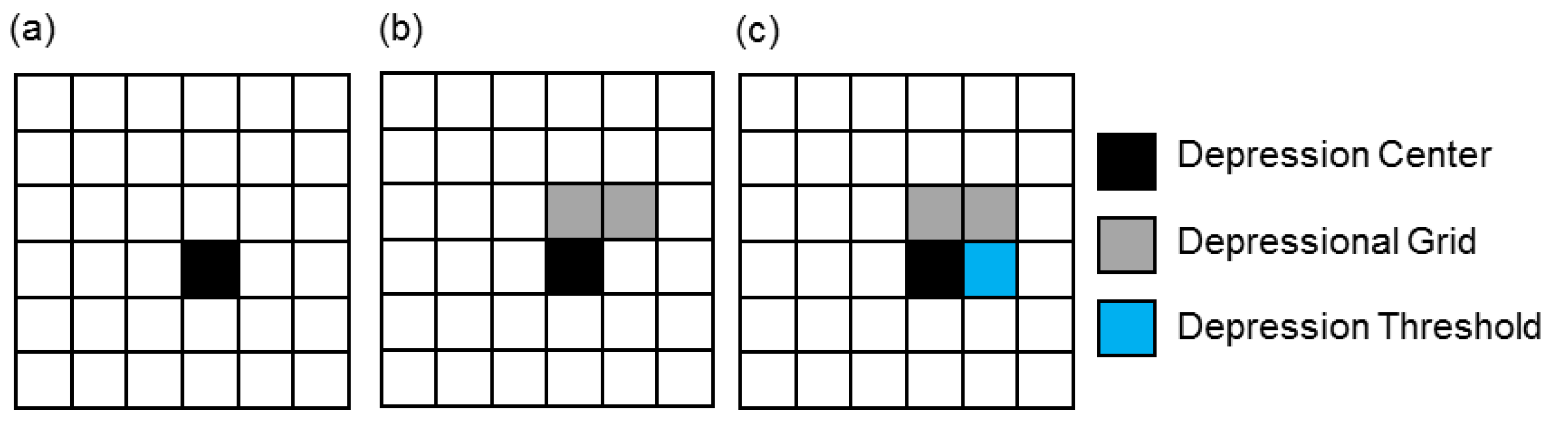
The puddle delineation (PD) algorithm [31] is employed to analyze surface topography and identify depressions. Based on the PD algorithm, each depression possesses two main elements: center and threshold [31]. The center grid has the lowest elevation among all depressional grids whereas the threshold grid has the highest elevation among depressional grids, over which the fully-filled depression spills. To identify a depression, PD locates its center grid, adds its depressional grids, and determines its threshold grid [31]. To locate centers, PD identifies local minima on the DEM surface (Figure 2a). It then searches for all depressional grids for each depression through a search list (Figure 2b), until a threshold grid is located (Figure 2c) [31].
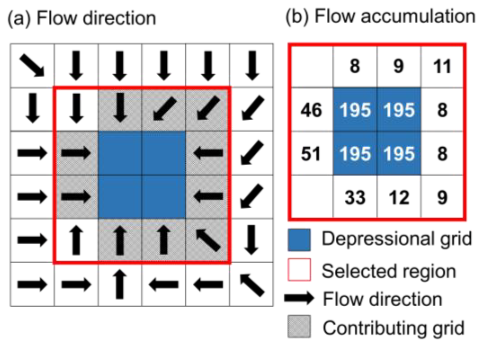
Flow directions are determined by using a modified D8 method [40] for the original DEM. Figure 3a depicts a schematic example of the modified D8 method for a sample surface. Specifically, the original D8 method assigns non-zero numbers to all DEM grids, which represent different flow directions. However, the modified D8 method is coupled with PD and allocates a “zero” flow direction to all grids associated with puddles [31] (Figure 3a). In other words, the depressional grids in a puddle do not have any flow direction (Figure 3a). When the flow direction matrix is completed for the entire surface, flow accumulation values are calculated for all grids. Each grid possesses a unique flow accumulation number, signifying the number of grids contributing surface runoff to it. However, the flow accumulation computation procedure for depressional grids is different. For depressional grids, the flow accumulation number is calculated based on the flow accumulation of all surrounding DEM grids that directly make runoff contributions to the puddle (highlighted cells in the red box on Figure 3a). All depressional grids residing in a puddle share the same flow accumulation value (Figure 3b). For example, as shown in Figure 3b, the identified depression/puddle (blue grids) has 10 contributing grids, each of which possesses a unique flow accumulation number. The summation of all these 10 flow accumulation values (46 + 51 + 33 + 12 + 9 + 8 + 8 + 11 + 9 + 8) equals 195 and is assigned as the flow accumulation to the four depressional grids in the depression/puddle (Figure 3b).
To achieve the objectives of this study, two methods of analysis were used. Spatial representations of the TWI values across the dendritic NE surface and the depression-dominated CLSA surface were depicted to highlight the differences in TWI computation procedures and the underlying methodology. Additionally, two statistical measures were utilized to investigate the distribution, spread, and clustering of TWI, tan(β), and ln(α) for the entire CLSA surface and depressional grids at different resolutions. To compare the frequency distributions of TWI across multiple DEM resolutions (1 m, 2.5 m, 5 m, 10 m, 20 m, and 30 m), each resolution was resampled to a 1-m resolution DEM. For example, each grid of a 30-m DEM is represented by 900 1-m grids. In this way, each resolution, after resampling, had a similar sample size.
3. Results
3.1. DEM Modification Based on Surveyed Bathymetry Data
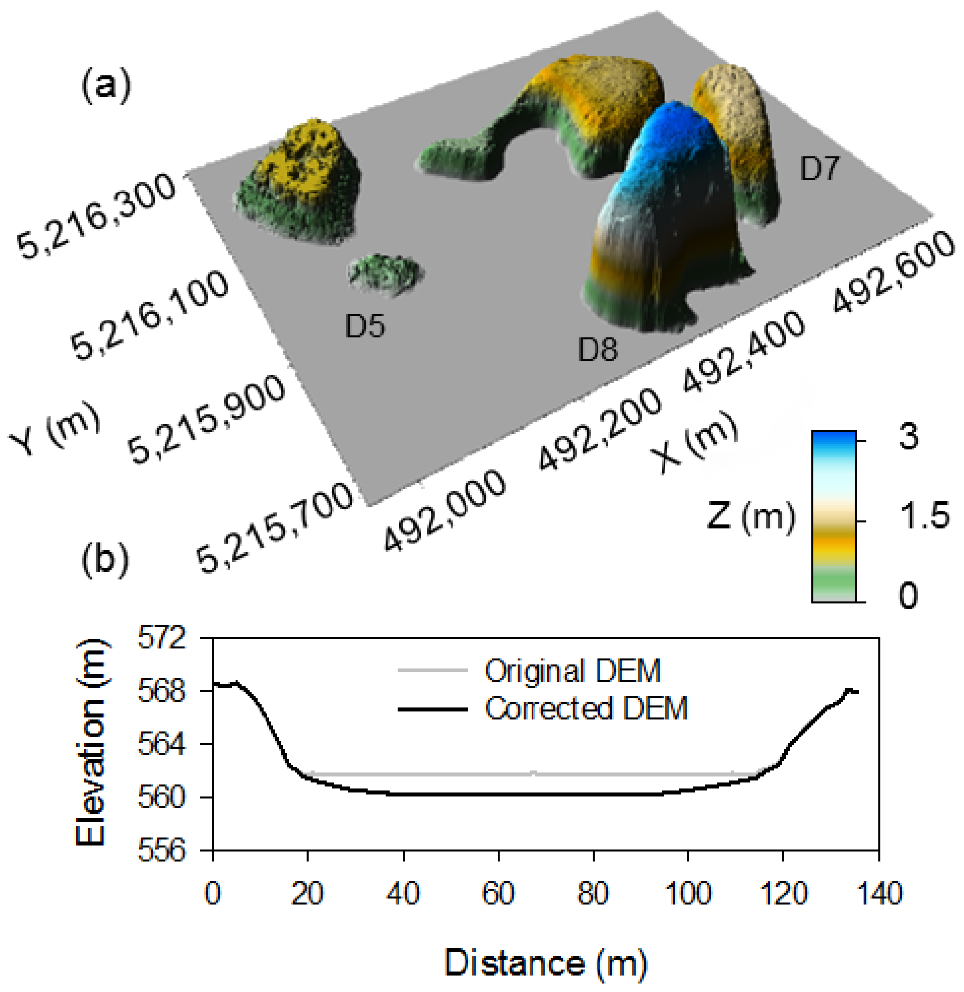
A comparison between the original 1-m DEM and the corrected 1-m DEM, which incorporated the pothole bathymetry for the CLSA surface, highlights the importance of depressions in topographic and hydrologic analyses. Figure 4a depicts the 3D distribution of the elevation differences between the original and corrected DEMs, and Figure 4b provides a detailed comparison of the selected cross-section a-b of depression D7 (Figure 1a). Correcting the original DEM by the pothole bathymetry resulted in a storage difference of 1.5 × 10⁵ m3 between the two DEMs. Depression D8 had the highest change in storage (6.7 × 10⁴ m3), while depression D5 showed the lowest change (718.3 m3). Figure 4a illustrates the distribution of these changes over the CLSA surface. It can be observed that the depths change up to 3 m (D8 in Figure 4a). As shown in Figure 4b, the original DEM reflects a flat, whereas the corrected DEM displays the distribution of the actual bed topography of the depression. The observed flat on the original DEM implies that the DEM was generated while the depression contained water. These marked changes suggest that caution should be taken when using currently available DEMs for depression-dominated areas, as depressions exist in abundance on those surfaces.
3.2. TWI Distribution for Dendritic and Depression-Dominated Surfaces
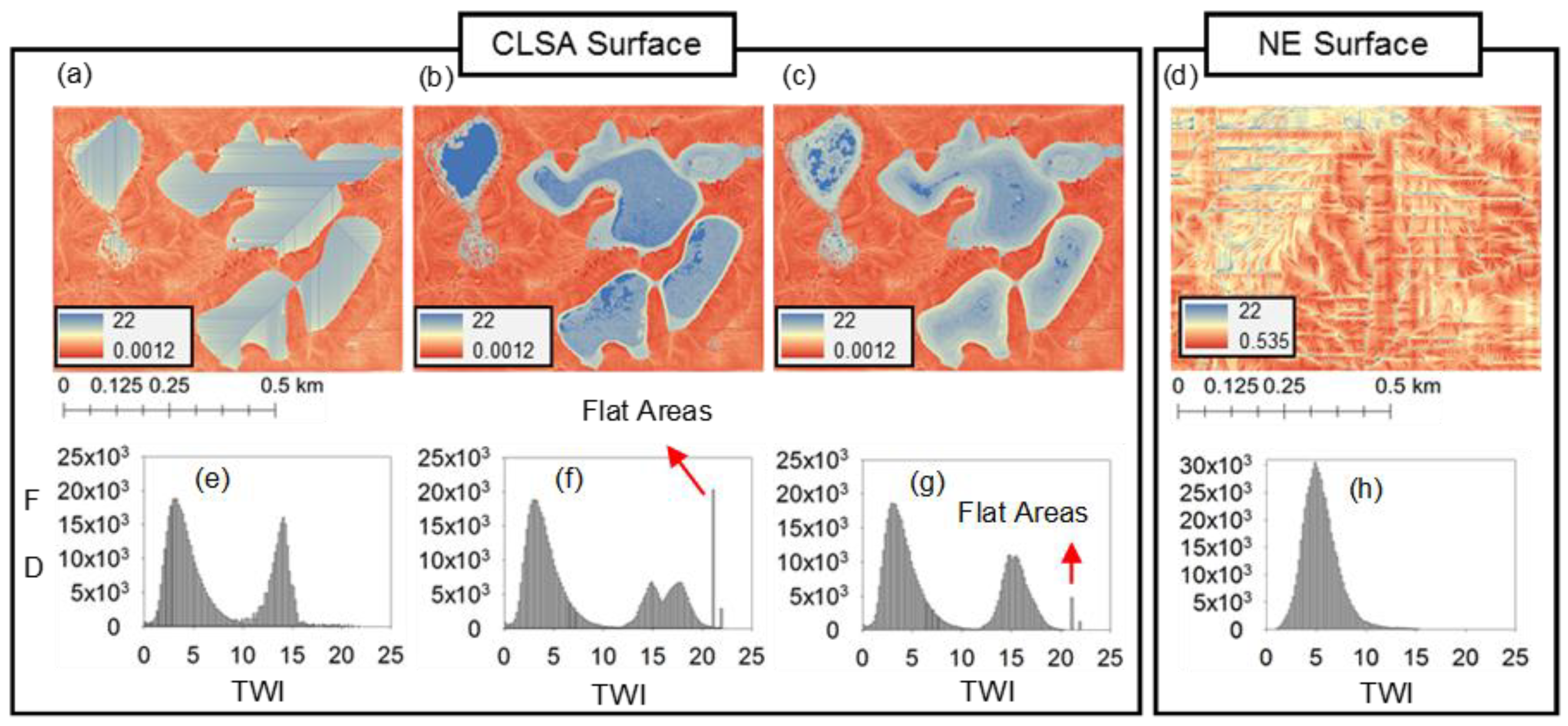
Figure 5a–c show the TWI results based on the 1-m resolution DEMs of the CLSA surface for three scenarios: (1) filled DEM; (2) original DEM; and (3) corrected DEM. Figure 5d displays the TWI computed by using the 1-m resolution DEM for the NE surface. Also, Figure 5e–h shows the frequency distribution functions of the CLSA and NE surfaces, which provide information on the distributions of TWI over different topographic surfaces in different scenarios. A visual comparison between the dendritic NE surface and the depression-dominated CLSA surface reveals the fundamental differences in TWI distributions. As expected, the highest TWI values were along channels for the NE surface (Figure 5d), whereas depressions had the highest TWI values for the CLSA surface (Figure 5a–c).
Analyses of different scenarios for the CLSA surface indicate that using the filled-DEM to compute TWI resulted in misleading values and distributions of TWI. As shown in Figure 5a, the highest TWI values were formed along the artificially-generated channels inside the filled depressions. This alteration of surface topography may facilitate hydrologic modeling by creating a well-connected drainage network, which changes the distribution of topographic indices inside the depressions. Figure 5b shows the TWI distribution computed by using the original DEM. Since the original DEM reflected depressions as flats, the TWI values for the grids inside a depression were almost the same. For example, the TWI value for the 14,569 grids in the flat over depression D6 was 21.18. Figure 5c suggests that correcting the original DEM led to an actual topography-based distribution of TWI. In other words, the depressional grids located in the centers of depressions had higher TWI values and, understandably, were more prone to saturation.
Moreover, the frequency distribution results disclose different patterns for the CLSA and NE surfaces (Figure 5e–h). The NE surface shows a one-hump distribution pattern, like other dendritic surfaces [10]; however, a two-hump distribution pattern can be observed for the depression-dominated CLSA surface (Figure 5). These different patterns can be attributed to the microtopographic differences between the two surfaces. The first hump in the frequency distribution of the CLSA surface represents all non-depressional grids, while the second hump reflects the effect of the abundance of depressions (Figure 5e–g).
Specifically, different scenarios for the CLSA surface led to significant changes in the distributions of TWI for the depressional grids (the second hump in Figure 5e–g). The TWI distribution results for the filled-DEM indicate that only 17,604 grids had TWI values greater than 15 (Figure 5e). This low frequency of higher TWI values was a direct consequence of the sink-filling preprocessing and introduction of artificially generated channels. For the original DEM, the second hump clearly shows that TWI values for the depressional grids were higher than those computed by using the filled-DEM. However, there are two sharp increases right after the second hump (Figure 5f). These sharp changes (representing 23,443 depressional grids with TWI values greater than 21.10) are associated with the presence of flats over depressions. Correcting the original DEM by using the bathymetry data helped to remove these flats and get the real bed-elevation distribution of the depressions. Figure 5g displays that sharp increases after the second hump decreased dramatically; however, even after correcting the original DEM, some flat areas still existed (e.g., P8 in Figure 5c). As discussed before, these flat areas are associated with vegetation in the high-resolution LiDAR data and can be eliminated by further processing.
3.3. Resolution Effects on TWI Distribution
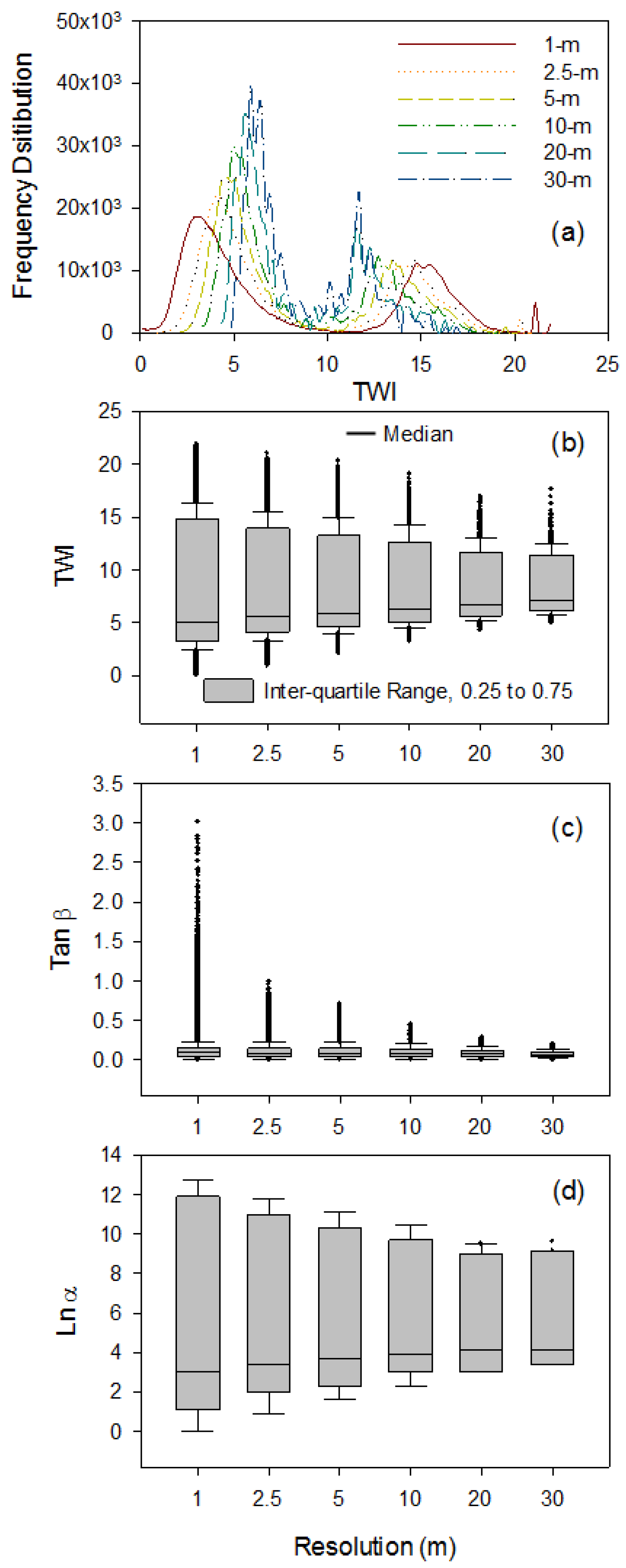
TWI, computed by using the modified procedure, also showed variations with DEM resolution. Generally, all resolutions (1 m, 2.5 m, 5 m, 10 m, 20 m, 30 m) displayed a frequency distribution of TWI with a two-hump pattern (Figure 6a), as previously highlighted in Figure 5. However, a higher resolution DEM reflected a larger range of TWI values (Figure 6a,b). As the grid size increased, the space between the first and second hump decreased (Figure 6a). This implies that coarse resolution DEMs displayed non-depressional grids and depressional grids with intermediate TWI values, rather than extreme TWI values as computed for the 1-m resolution. In Figure 6b the range of data between the 25th and 75th percentiles decreased with increasing the DEM grid size. This supports what was observed in Figure 6a. In other words, coarse resolution DEMs had higher TWIs for non-depressional grids and lower TWIs for depressional grids when compared with fine resolution DEMs. Therefore, according to the TWI values for the resolutions selected in this study, non-depressional grids in coarse resolution DEMs were more apt to saturation, and depressional grids were less apt to saturation.
Figure 6b shows the statistical summary of TWI values across the entire CLSA surface for all resolutions. The median TWI rose from 5.11 to 7.11 for the 1-m and 30-m resolutions, respectively. The mean TWI value also rose from 8.19 to 8.53 with increasing DEM grid size from 1 m to 30 m, respectively. This increase in mean TWI with increasing DEM grid size is consistent with TWI observations in the study done by Saulnier et al. [12]. Between the 25th and 75th percentiles, TWI values ranged from 3.27 to 14.77 for the 1-m DEM and from 6.16 to 11.41 for the 30-m DEM. The distributions for all resolutions, however, were skewed right, indicating that 50% of the TWI values were clustered around low TWI values, whereas the remaining 50% of the TWI values were spread out over a larger range, from 5.11 to 21.92 for the 1-m resolution and from 7.11 to 17.63 for the 30-m resolution.
Figure 6c depicts the statistical summary of slope tan(β) for the entire CLSA surface for all selected resolutions. It can be observed that skewness decreased with increasing DEM grid size. In other words, the slopes became smoother with increasing grid size (smoothing effect), which is expected as shown in other studies (e.g., [19]). However, the range of tan(β) for the 1-m DEM was almost 15 times larger than that for the 30-m DEM. As discussed in the methodology, the high-resolution LiDAR data depict the presence of vegetation that can affect the slope calculations. The median and mean of tan(β) values were almost the same with increasing grid size, which is consistent with the results of Sørensen and Seibert [14]. Figure 6d shows the statistical summary of upslope contributing area, ln(α), for the entire CLSA surface for all resolutions. Similar to the TWI range in Figure 6b, the range of contributing area decreased with increasing DEM grid size. The median and mean values increased with increasing grid size, from 2.99 and 5.54 for the 1-m resolution to 4.09 and 5.62 for the 30-m resolution, respectively. As previous studies suggested, upslope contributing area dominates the computation of TWI [2,14]. This study also confirmed that changing DEM resolution from fine to coarse led to a decrease in TWI range, which is a direct consequence of the decreasing pattern of ln(α).
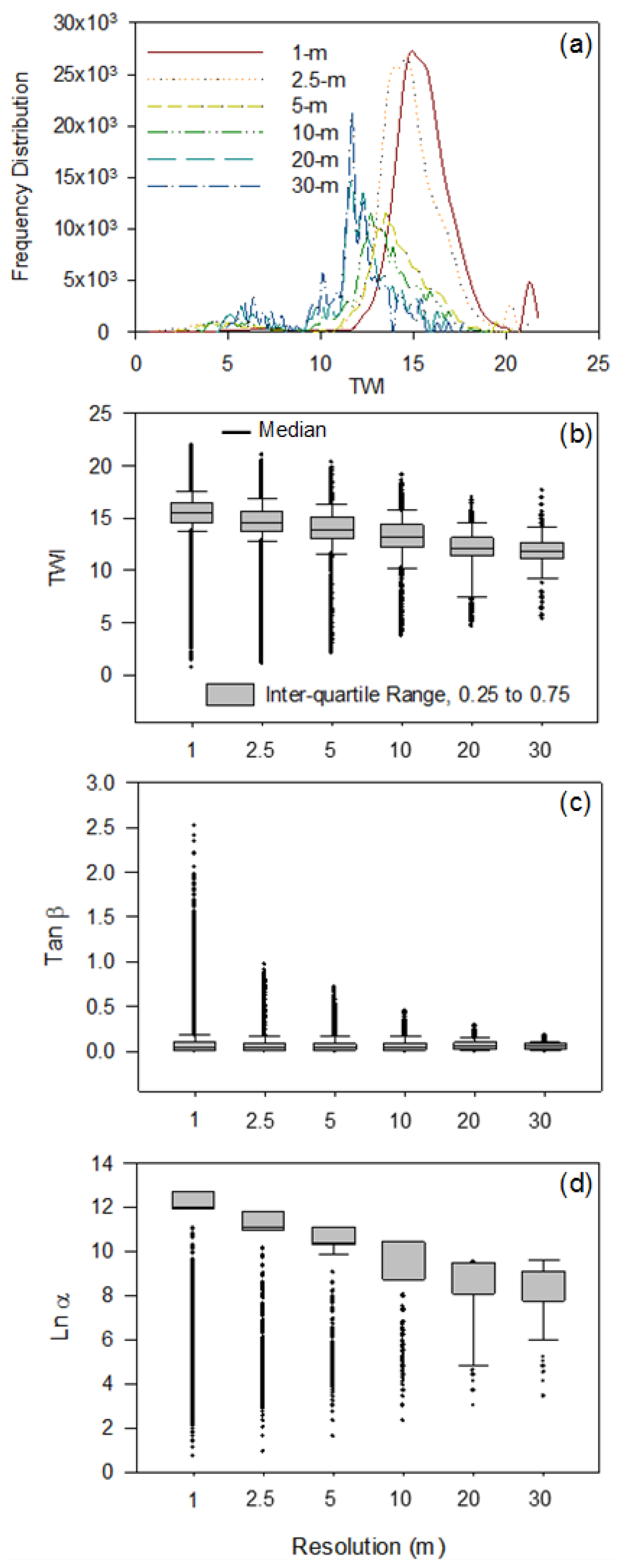
To investigate the effects of the modified TWI computation procedure for depression-dominated areas, it is also important to take a closer look at TWI, tan(β), and ln(α) calculated solely for depressional grids (Figure 7a–d). Figure 7a depicts the frequency distribution of TWI values of the depressional grids for the six different resolutions. Comparing the results from different DEM resolutions side by side demonstrated that the majority of depressional grids for coarser resolutions were less likely to be saturated, which can be attributed to the fact that the frequency peaks occurred at lower TWI values. Figure 7a (similar to Figure 6a) shows that TWI is sensitive to the changes in resolution, which is parallel with various studies on the resolution effect on TWI. However, the statistical summary of the TWI values of depressional grids for all resolutions (Figure 7b) indicates that the mean values decreased with increasing grid size. This new finding is specific to depression-dominated areas, as other studies focused on TWI in dendritic watersheds (e.g., [12]). The median and mean of TWI decreased with increasing DEM grid size, from 15.43 and 15.56 for the 1-m resolution to 11.77 and 11.67 for the 30-m resolution, respectively. This is opposite to what was observed for the mean and median TWI values for the entire CLSA surface (Figure 6b). These box plots are skewed left, indicating that 50% of the data points are located on the high end of the TWI scale. This finding is in accordance with what is to be expected (i.e., high TWI values for depressional grids).
The values of tan(β) for different resolutions in Figure 7c resemble the general trend in Figure 6c. This means that the mean and median of tan(β) for different resolutions stayed almost constant for depressional grids. For example, the difference between the median values for the 1-m and 30-m resolution DEMs was only 0.01. Figure 7d depicts the upslope contributing area, ln(α), of depressional grids. The box plots indicate that 50% of the data points between the 25th and 75th percentiles had a high contributing area for depressional grids. Due to the modified procedure for calculating α, depressional grids were expected to have large contributing areas and be limited to a small range of ln(α) values between the 25th and 75th percentiles. Unlike ln(α) for the entire CLSA surface (Figure 6d), ln(α) for depressional grids followed a decreasing pattern with increasing grid size. For example, the mean value of ln(α) fell from 12.17 to 8.41 by increasing DEM grid size from 1 m to 30 m, respectively. Similar to other studies [2,14], our results for the whole surface indicate that ln(α) dominates the computation of TWI, but exhibits a decreasing trend with increasing DEM grid size.
4. Conclusions
Previous studies have focused on the computation of TWI for typical dendritic land surfaces. Due to the underlying limitations in calculating slopes and flow accumulations based on depressionless DEMs from sink-filling pre-processing, traditional TWI computation methodologies cannot depict accurate TWI values for depression-dominated areas. A modified TWI computation procedure was proposed in this study, particularly for depression-dominated areas. In addition, a corrected DEM was generated to reflect the bathymetry of potholes where the original DEM showed the water surface elevations (i.e., flats). A two-hump frequency distribution of TWI computed by using the modified procedure was identified for depression-dominated areas, whereas typical dendritic surfaces showed a one-hump distribution, as previously observed in other studies. The TWI computation based on the original DEM indicated peaks after the second hump, showing the presence of flats. However, the TWI computation for the corrected DEM led to fewer flat areas.
Changing DEM resolution also impacted TWI computations. Statistical summaries were provided for both depressional grids and all grids over the entire surface. Clear trends were observed for TWI, tan(β), and ln(α). Specifically, the mean of TWI increased from 8.19 for the 1-m DEM to 8.53 for the 30-m DEM. However, depressional grids experienced a decrease in the mean TWI values, from 15.57 to 11.67 with decreasing resolution from 1 m to 30 m. The mean values of tan(β) for the entire surface and depressional grids remained relatively constant, whereas ln(α) for the entire surface and depressional grids had an opposite trend. This finding suggests that ln(α) dominates the computations of TWI for depressional grids.
The results demonstrated that currently available DEMs failed to capture actual topography of depression-dominated areas, which could lead to misleading values of TWI, which can further impact the hydrologic modeling relating to runoff generation. Specifically, the methodology and findings from this study can also be applied to modeling the hydrologic response of surfaces in the PPR or other depression-dominated surfaces around the world.
Author Contributions
All authors contributed equally to this work, including the related research and writing.
Acknowledgments
This material is based upon work supported by the National Science Foundation under Grant No. NSF EPSCoR Award IIA-1355466. The North Dakota Water Resources Research Institute also provided partial financial support in the form of a graduate fellowship for the first and second authors. Authors would like to thank Jamal Ghauri, Jackie Arntson, and Dillon Ekholm for their contributions to the related research.
Conflicts of Interest
The authors declare no conflict of interest. The founding sponsors had no role in the design of the study; in the collection, analyses, or interpretation of data; in the writing of the manuscript, and in the decision to publish the results.
References
- Beven, K.J.; Kirkby, M.J. A physically based, variable contributing area model of basin hydrology/Un modèle à base physique de zone d’appel variable de l’hydrologie du bassin versant. Hydrol. Sci. Bull. 1979, 24, 43–69. [Google Scholar] [CrossRef]
- Hjerdt, K.N.; Mcdonnell, J.J.; Seibert, J.; Rodhe, A. A new topographic index to quantify downslope controls on local drainage. Water Resour. Res. 2004, 40, 1–6. [Google Scholar] [CrossRef]
- Chu, X. Delineation of Pothole-Dominated Wetlands and Modeling of Their Threshold Behaviors. J. Hydrol. Eng. 2015, D5015003. [Google Scholar] [CrossRef]
- Zinko, U.; Seibert, J.; Dynesius, M.; Nilsson, C. Plant Species Numbers Predicted by a Topography-based Groundwater Flow Index. Ecosystems 2005, 8, 430–441. [Google Scholar] [CrossRef]
- Bernier, P.Y. Variable source areas and storm-flow generation: An update of the concept and a simulation effort. J. Hydrol. 1985, 79, 195–213. [Google Scholar] [CrossRef]
- Lyon, S.W.; Walter, M.T.; Gérard-Marchant, P.; Steenhuis, T.S. Using a topographic index to distribute variable source area runoff predicted with the SCS curve-number equation. Hydrol. Process. 2004, 18, 2757–2771. [Google Scholar] [CrossRef]
- Beven, K.J.; Kirkby, M.J.; Schofield, N.; Tagg, A.F. Testing a physically-based flood forecasting model (TOPMODEL) for three U.K. catchments. J. Hydrol. 1984, 69, 119–143. [Google Scholar] [CrossRef]
- Hornberger, G.M.; Beven, K.J.; Cosby, B.J.; Sappington, D.E. Shenandoah Watershed Study: Calibration of a Topography-Based, Variable Contributing Area Hydrological Model to a Small Forested Catchment. Water Resour. Res. 1985, 21, 1841–1850. [Google Scholar] [CrossRef]
- Quinn, P.F.; Beven, K.J. Spatial and temporal predictions of soil moisture dynamics, runoff, variable source areas and evapotranspiration for plynlimon, mid-wales. Hydrol. Process. 1993, 7, 425–448. [Google Scholar] [CrossRef]
- Quinn, P.F.; Beven, K.J.; Lamb, R. The in(a/tan/β) index: How to calculate it and how to use it within the topmodel framework. Hydrol. Process. 1995, 9, 161–182. [Google Scholar] [CrossRef]
- Hancock, G.R. The use of digital elevation models in the identification and characterization of catchments over different grid scales. Hydrol. Process. 2005, 19, 1727–1749. [Google Scholar] [CrossRef]
- Saulnier, G.; Obled, C.; Beven, K. Analytical compensation between DTM grid resolution and effective values of saturated hydraulic conductivity within the TOPMODEL framework. Hydrol. Process. 1997, 11, 1331–1346. [Google Scholar] [CrossRef]
- Vaze, J.; Teng, J.; Spencer, G. Impact of DEM accuracy and resolution on topographic indices. Environ. Model. Softw. 2010, 25, 1086–1098. [Google Scholar] [CrossRef]
- Sørensen, R.; Seibert, J. Effects of DEM resolution on the calculation of topographical indices: TWI and its components. J. Hydrol. 2007, 347, 79–89. [Google Scholar] [CrossRef]
- Wolock, D.M.; McCabe, G.J. Differences in topographic characteristics computed from 100- and 1000-m resolution digital elevation model data. Hydrol. Process. 2000, 14, 987–1002. [Google Scholar] [CrossRef]
- Fisher, P.F.; Tate, N.J. Causes and consequences of error in digital elevation models. Prog. Phys. Geogr. 2006, 30, 467–489. [Google Scholar] [CrossRef]
- Temme, A.J.A.M.; Schoorl, J.M.; Veldkamp, A. Algorithm for dealing with depressions in dynamic landscape evolution models. Comput. Geosci. 2006, 32, 452–461. [Google Scholar] [CrossRef]
- Chu, X.; Yang, J.; Chi, Y.; Zhang, J. Dynamic puddle delineation and modeling of puddle-to-puddle filling-spilling-merging-splitting overland flow processes. Water Resour. Res. 2013, 49, 3825–3829. [Google Scholar] [CrossRef]
- Habtezion, N.; Tahmasebi Nasab, M.; Chu, X. How does DEM resolution affect microtopographic characteristics, hydrologic connectivity, and modelling of hydrologic processes? Hydrol. Process. 2016, 30, 4870–4892. [Google Scholar] [CrossRef]
- Tahmasebi Nasab, M.; Jia, X.; Chu, X. Modeling of Subsurface Drainage under Varying Microtopographic, Soil and Rainfall Conditions. In 10th International Drainage Symposium; Strock, J., Ed.; American Society of Agricultural and Biological Engineers: Minneapolis, MN, USA, 2016; pp. 133–138. [Google Scholar]
- Tahmasebi Nasab, M.; Grimm, K.; Wang, N.; Chu, X. Scale Analysis for Depression-Dominated Areas: How Does Threshold Resolution Represent a Surface. In World Environmental and Water Resources Congress 2017; American Society of Civil Engineers: Reston, VA, USA, 2017; pp. 164–174. [Google Scholar]
- Tahmasebi Nasab, M.; Singh, V.; Chu, X. SWAT Modeling for Depression-Dominated Areas: How Do Depressions Manipulate Hydrologic Modeling? Water 2017, 9, 58. [Google Scholar] [CrossRef]
- Tahmasebi Nasab, M.; Zhang, J.; Chu, X. A New Depression-Dominated Delineation (D-cubed) Method for Improved Watershed Modeling. Hydrol. Process. 2017, 31, 3364–3378. [Google Scholar] [CrossRef]
- Garbrecht, J.; Campbell, J. An Automated Digital Landscape Analysis Tool for Topographic Evaluation, Drainage Identification, Watershed Segmentation and Subcatchment Parameterization: TOPAZ User Manual; USDA, Agricultural Research Service, Grazinglands Research Laboratory: El Reno, OK, USA, 1997.
- Jenson, S.K.; Domingue, J.O. Extracting Topographic Structure from Digital Elevation Data for Geographic Information System Analysis. Photogramm. Eng. Remote Sens. 1988, 54, 1593–1600. [Google Scholar]
- Marks, D.; Dozier, J.; Frew, J. Automated Basin Delineation from Digital Terrain Data; NASA Goddard Space Flight Center: Greenbelt, MD, USA, 1983.
- Martz, L.W.; Garbrecht, J. The treatment of flat areas and depressions in automated drainage analysis of raster digital elevation models. Hydrol. Process. 1998, 12, 843–855. [Google Scholar] [CrossRef]
- O’Callaghan, J.F.; Mark, D.M. The extraction of drainage networks from digital elevation data. Comput. Vis. Graph. Image Process. 1984, 28, 323–344. [Google Scholar] [CrossRef]
- Barnes, R.; Lehman, C.; Mulla, D. An efficient assignment of drainage direction over flat surfaces in raster digital elevation models. Comput. Geosci. 2014, 62, 128–135. [Google Scholar] [CrossRef]
- Nardi, F.; Grimaldi, S.; Santini, M.; Petroselli, A.; Ubertini, L. Hydrogeomorphic properties of simulated drainage patterns using digital elevation models: The flat area issue/Propriétés hydro-géomorphologiques de réseaux de drainage simulés à partir de modèles numériques de terrain: La question des zones planes. Hydrol. Sci. J. 2008, 53, 1176–1193. [Google Scholar] [CrossRef]
- Chu, X.; Zhang, J.; Chi, Y.; Yang, J. An Improved Method for Watershed Delineation and Computation of Surface Depression Storage. In Watershed Management 2010; American Society of Civil Engineers: Reston, VA, USA, 2010; pp. 1113–1122. [Google Scholar]
- Schmidt, F.; Persson, A. Comparison of DEM Data Capture and Topographic Wetness Indices. Precis. Agric. 2003, 4, 179–192. [Google Scholar] [CrossRef]
- Winter, T.C. Hydrological, Chemical, and Biological Characteristics of a Prairie Pothole Wetland Complex under Highly Variable Climate Conditions: The Cottonwood Lake Area, East-Central North Dakota; U.S. Dept. of the Interior, U.S. Geological Survey: Reston, VA, USA, 2003.
- United States Geological Survey (USGS). National Map Viewer. Available online: https://viewer.nationalmap.gov/basic/ (accessed on 3 May 2017).
- SonTek. SonTek—RiverSurveyor S5 and M9. Available online: http://www.sontek.com/ (accessed on 2 May 2017).
- Quinn, P.; Beven, K.; Chevallier, P.; Planchon, O. The prediction of hillslope flow paths for distributed hydrological modelling using digital terrain models. Hydrol. Process. 1991, 5, 59–79. [Google Scholar] [CrossRef]
- Sørensen, R.; Zinko, U.; Seibert, J. On the calculation of the topographic wetness index: Evaluation of different methods based on field observations. Hydrol. Earth Syst. Sci. 2006, 10, 101–112. [Google Scholar] [CrossRef] [Green Version]
- Tarboton, D.G. A new method for the determination of flow directions and upslope areas in grid digital elevation models. Water Resour. Res. 1997, 33, 309–319. [Google Scholar] [CrossRef]
- Wolock, D.M.; McCabe, G.J. Comparison of Single and Multiple Flow Direction Algorithms for Computing Topographic Parameters in TOPMODEL. Water Resour. Res. 1995, 31, 1315–1324. [Google Scholar] [CrossRef]
- Garbrecht, J.; Martz, L.W. The assignment of drainage direction over flat surfaces in raster digital elevation models. J. Hydrol. 1997, 193, 204–213. [Google Scholar] [CrossRef]
Figure 1.
Geographical locations of the Prairie Pothole Region (PPR) and the two selected sites: (a) Cottonwood Lake Study Area (CLSA) surface (D denotes major depressions on the surface) and (b) Nelson Eddy (NE) surface near the border of Nelson and Eddy Counties.
Figure 1.
Geographical locations of the Prairie Pothole Region (PPR) and the two selected sites: (a) Cottonwood Lake Study Area (CLSA) surface (D denotes major depressions on the surface) and (b) Nelson Eddy (NE) surface near the border of Nelson and Eddy Counties.

Figure 2.
Identification of depressional elements in the puddle delineation (PD) algorithm: (a) center grid; (b) depressional grids; and (c) threshold grid.
Figure 2.
Identification of depressional elements in the puddle delineation (PD) algorithm: (a) center grid; (b) depressional grids; and (c) threshold grid.

Figure 3.
Schematic representation of (a) flow direction and (b) flow accumulation for a depression/puddle.
Figure 3.
Schematic representation of (a) flow direction and (b) flow accumulation for a depression/puddle.

Figure 4.
(a) 3D distribution of the elevation differences between the original digital elevation model (DEM) and the corrected DEM that incorporates the pothole bathymetry data; (b) comparison between the two DEMs for a cross-section of depression D7.
Figure 4.
(a) 3D distribution of the elevation differences between the original digital elevation model (DEM) and the corrected DEM that incorporates the pothole bathymetry data; (b) comparison between the two DEMs for a cross-section of depression D7.

Figure 5.
Visual comparisons of topographic wetness index (TWI) computations (a-d) and frequency distributions (FD) (e-h) for two different surfaces: depression-dominated Cottonwood Lake Study Area (CLSA) surface (a–c) and dendritic Nelson Eddy (NE) surface (d); TWI values were calculated for the CLSA surface based on (a) filled DEM; (b) original DEM; and (c) corrected DEM.

Figure 6.
Frequency distribution of TWI (a) and statistical summary of TWI (b), tan(β) (c), and ln(α) (d) for 1-m, 2.5-m, 5-m, 10-m, 20-m, and 30-m resolutions of the entire Cottonwood Lake Study Area (CLSA) surface using the modified TWI procedure.
Figure 6.
Frequency distribution of TWI (a) and statistical summary of TWI (b), tan(β) (c), and ln(α) (d) for 1-m, 2.5-m, 5-m, 10-m, 20-m, and 30-m resolutions of the entire Cottonwood Lake Study Area (CLSA) surface using the modified TWI procedure.

Figure 7.
Frequency distribution of TWI (a) and statistical summary of TWI (b), tan(β) (c), and ln(α) (d) for 1-m, 2.5-m, 5-m, 10-m, 20-m, and 30-m resolutions of depressional grids on the Cottonwood Lake Study Area (CLSA) surface using the modified TWI procedure.
Figure 7.
Frequency distribution of TWI (a) and statistical summary of TWI (b), tan(β) (c), and ln(α) (d) for 1-m, 2.5-m, 5-m, 10-m, 20-m, and 30-m resolutions of depressional grids on the Cottonwood Lake Study Area (CLSA) surface using the modified TWI procedure.

© 2018 by the authors. Licensee MDPI, Basel, Switzerland. This article is an open access article distributed under the terms and conditions of the Creative Commons Attribution (CC BY) license (http://creativecommons.org/licenses/by/4.0/).
Share and Cite
MDPI and ACS Style
Grimm, K.; Tahmasebi Nasab, M.; Chu, X. TWI Computations and Topographic Analysis of Depression-Dominated Surfaces. Water 2018, 10, 663. https://doi.org/10.3390/w10050663
AMA Style
Grimm K, Tahmasebi Nasab M, Chu X. TWI Computations and Topographic Analysis of Depression-Dominated Surfaces. Water. 2018; 10(5):663. https://doi.org/10.3390/w10050663
Chicago/Turabian StyleGrimm, Kendall, Mohsen Tahmasebi Nasab, and Xuefeng Chu. 2018. "TWI Computations and Topographic Analysis of Depression-Dominated Surfaces" Water 10, no. 5: 663. https://doi.org/10.3390/w10050663
Note that from the first issue of 2016, this journal uses article numbers instead of page numbers. See further details here.