Article

Simulation of Soil Water Content in Mediterranean Ecosystems by Biogeochemical and Remote Sensing Models

1
IBIMET-CNR, 50019 Sesto Fiorentino (FI), Italy
2
LaMMA Consortium, 50019 Sesto Fiorentino (FI), Italy
3
Department of Life Sciences, University of Siena, 53100 Siena, Italy
*
Author to whom correspondence should be addressed.
Water 2018, 10(5), 665; https://doi.org/10.3390/w10050665
Submission received: 14 March 2018 / Revised: 10 May 2018 / Accepted: 16 May 2018 / Published: 19 May 2018
(This article belongs to the Special Issue Monitoring and Predicting Soil Moisture and Drought Conditions)

Abstract

:
The current study assesses the potential of two modeling approaches to simulate the daily site water budget in Mediterranean ecosystems. Both models utilize a simplified one-bucket approach but are fed with different drivers. The first model, BIOME-BGC, simulates all main biogeochemical fluxes based on conventional meteorological and ancillary data, while the second uses evapotranspiration estimates derived from the combination of meteorological data and satellite normalized difference vegetation index (NDVI) images. The two models were tested for three Italian sites which are characterized by different vegetation types and ecoclimatic conditions: (i) low mountain coniferous forest; (ii) hilly deciduous forest; (iii) urban grassland. The soil water balance simulated by the two models was evaluated through comparison with daily measurements of soil water content (SWC) taken during a growing season. Satisfactory results were obtained in all cases by both approaches; the SWC estimates are significantly correlated with the measurements (correlation coefficient, r, higher than 0.74), and the mean errors are lower than 0.079 cm3 cm−3. The second model, however, generally shows a higher accuracy, which is dependent on the quality of the NDVI data utilized (r higher than 0.79 and errors lower than 0.059 cm3 cm−3). The study therefore provides useful indications for the application of these and similar simulation methods in different environmental situations.

1. Introduction

The availability of water affects a great number of biological and ecological processes, such as seed germination, plant growth and nutrition, and organic matter decomposition. In most terrestrial ecosystems, the amount of and seasonal variation in the available water are the most relevant factors determining the health and efficiency of living organisms, generally expressed by macroscopic elements, such as vegetation growth, biomass, fructification, and biocenosis composition. The available water is strictly related to the soil water content (SWC), whose assessment is increasingly adopted in land-use planning, especially at the watershed scale for the estimation of runoff and soil erosion [1]. In agriculture, such assessment supports irrigation scheduling and promises to be a way to rationalize conflicting water uses during the most critical periods. The assessment of SWC is particularly important in Mediterranean areas, which are characterized by marked water shortage during the warm season, leading to increasing conflicts among different economic sectors and problems related to forthcoming climatic changes [2].
Numerous methodologies have been developed to assess SWC at different spatial and temporal scales. Some of them directly measure the amount of water as a fraction of total soil weight (i.e., gravimetric method) but are destructive and time consuming. Indirect methods have therefore been developed which relate soil water content to other variables (i.e., dielectric or heat flux sensors) [3]. All these methods, however, provide point measurements of SWC, whose extension over wider areas can be complicated by the spatial heterogeneity of controlling environmental factors (meteorology, terrain morphology, soil and vegetation features, etc.).
The modeling of SWC over larger areas must therefore account for these factors using information derived from various sources. Among the meteorological variables, temperature, rainfall, and solar radiation are the most influential on SWC, determining the direct input of water to the system and loss through potential evapotranspiration (ET0) [1]. Depending on the spatial scale of the investigation, these data can be locally collected by ground meteorological stations or derived from global data sets. Soil characteristics regulate water movement within layers and directly affect water retention, depending on particle size and porosity, as well as on organic content. All these features are extremely variable in space, mostly depending on the main pedogenetic factors, such as lithology, physiography, climate, vegetation, and others. The vegetation cover affects the soil water holding capacity of the decomposing materials in the litter and regulates the water loss through transpiration. The most interesting plant characteristics are therefore plant type and density, rooting system, canopy conductance, among others. These features are also characterized by an extreme spatial variability, which complicates the assessment of actual evapotranspiration (ETA) over large areas [1].
The integration of all these information types for the simulation of site water balance and SWC can be carried out by different modeling approaches. Hydrological models focus on the behavior of water in the underground layers and require detailed information on both soil and aquifers, which is often not available at the desired spatial and temporal scales [4]. Moreover, these models are generally suboptimal to simulate the water flux through the vegetation component of the ecosystems, particularly plant transpiration. An alternative is provided by biogeochemical and ecohydrological models, which integrate information on all ecosystem components to simulate the main fluxes through vegetation and soil [5,6]. BIOME-BGC is one of the most widespread of these models, being able to work at different spatial and temporal scales, using a minimum number of drivers and input data sets [7].
Remote sensing-based methods have also been largely applied to provide information on ecosystem status and processes. Synthetic aperture radar (SAR) imagery is potentially informative on SWC, but with variable spatial resolution and accuracy depending on several environmental features (e.g., [8,9,10]). Low spatial resolution satellite images can be also used for estimating several meteorological variables [11] (http://oiswww.eumetsat.org/IPPS/html/MSG/PRODUCTS/MPE). Finally, optical images taken by several sensors can provide information on vegetation quantity and condition, which can be integrated with ancillary data to simulate site water balance and SWC at different spatial and temporal scales [12]. The simplest methods which use remote sensing data to simulate plant water loss are based on the concept of crop coefficient (Kc). The Kc of each vegetation type, defined as the ratio between measured ETA and ET0 [13], is derived from vegetation indices, which express the quantity and status of vegetation. This approach has been successfully applied in irrigated agricultural areas, but generally tends to overestimate transpiration in cases of water limitation [14]. A new operational method that combines meteorological and normalized difference vegetation index (NDVI) data has been recently proposed by [15] to address this issue. The method (called NDVI-Cws) overcomes the tendency to overestimate ETA by the consideration of a short-term water stress scalar and has been successfully tested in Mediterranean areas.
The current paper aims at assessing the effectiveness of two modeling approaches for the simulation of the site water balance and SWC under different Mediterranean conditions. The first model is BIOME-BGC, which has been widely applied in the study region and estimates SWC through a simple one-bucket approach driven by conventional meteorological data. The second model feeds the same one-bucket approach with evapotranspiration estimates obtained through the NDVI-Cws method. The performances of the two models are evaluated versus field measurements of SWC taken in three Italian sites that are representative of different Mediterranean ecosystems (broadleaved and coniferous forests and grassland).

2. Materials and Methods
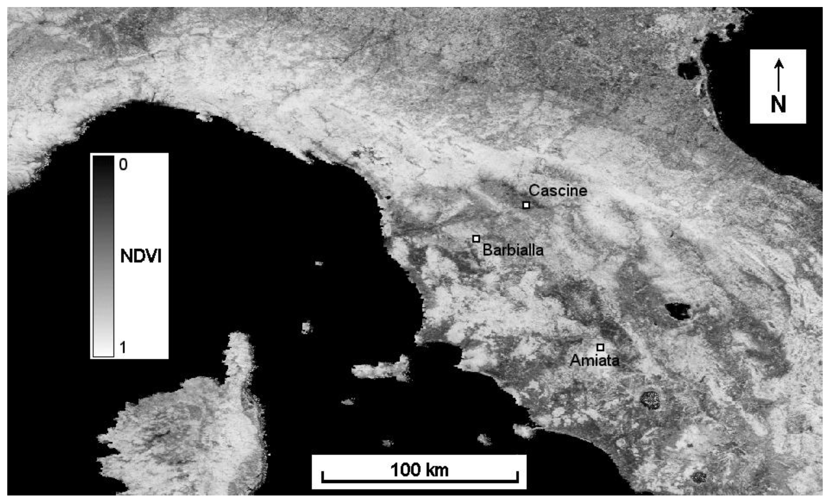
2.1. Study Sites

Three experimental sites were chosen in Tuscany, Central Italy (Figure 1), which, for their geographic, environmental and edaphic characteristics, are representative of different Mediterranean ecosystem types and drought risk conditions (Table 1). The main features of these sites can be summarized as follows:
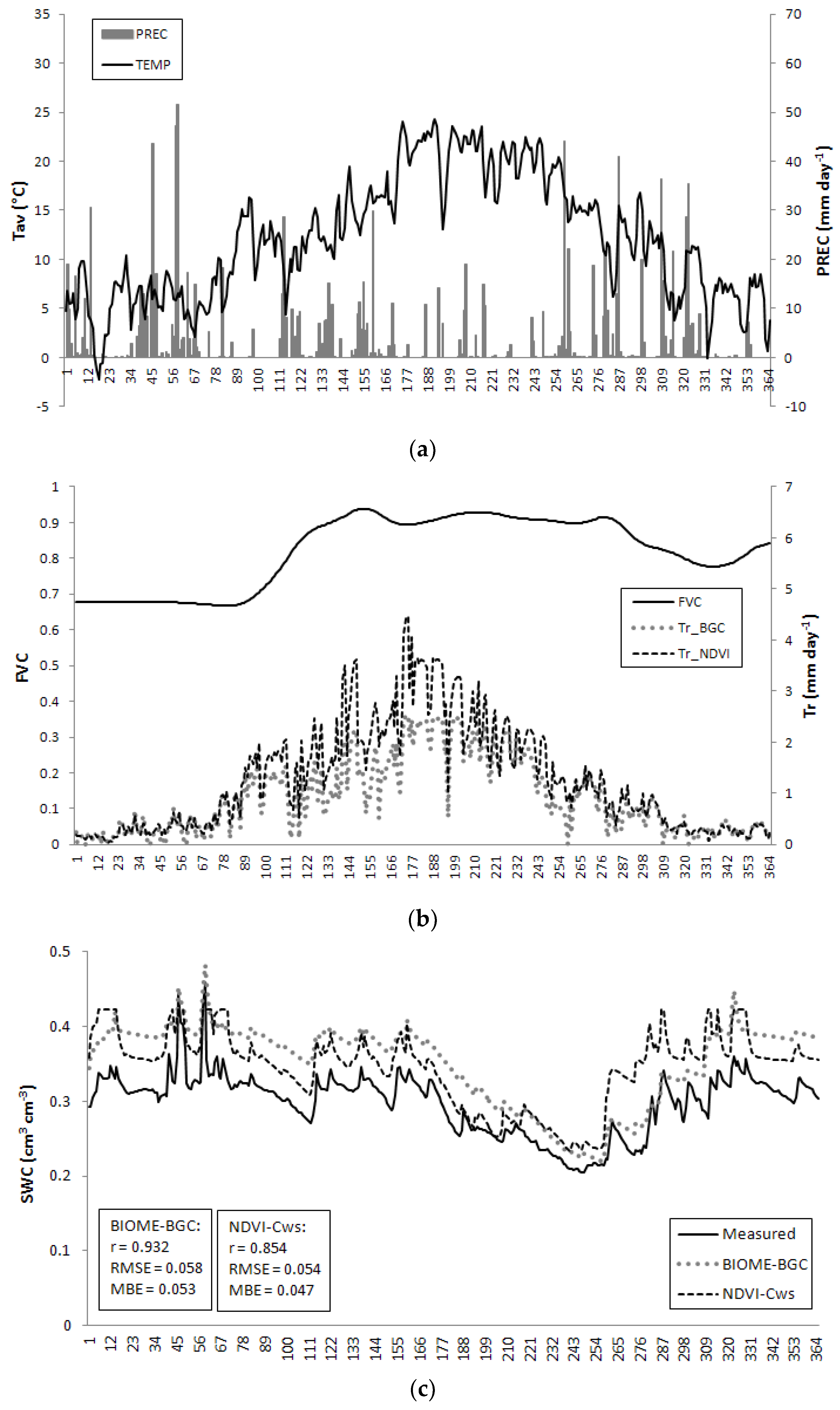
  • Barbialla (43.5917° N, 10.8486° E) is situated in a gently sloped terraced area, at 135 m. The mean annual rainfall is 810 mm and the mean annual temperature is around 15.1 °C. The coolest months are January and February (6.0 °C), while the hottest is August (25.1 °C). The vegetation cover is quite homogeneous (over 2 ha) and is dominated by hornbeam (Ostrya carpinifolia Scop.), poplar (Populus alba L.), and various oaks (Quercus cerris L., Q. pubescens L., Q. ilex L.). The soil surface is covered by native herbaceous vegetation and a few small shrub communities, among which are Cornus mas, C. sanguinea, and Crataegus monogyna. Soil is over 1 m deep, prevalently sandy, and has a field capacity of around 0.32 cm3 cm−3 (Table 2) [16,17].
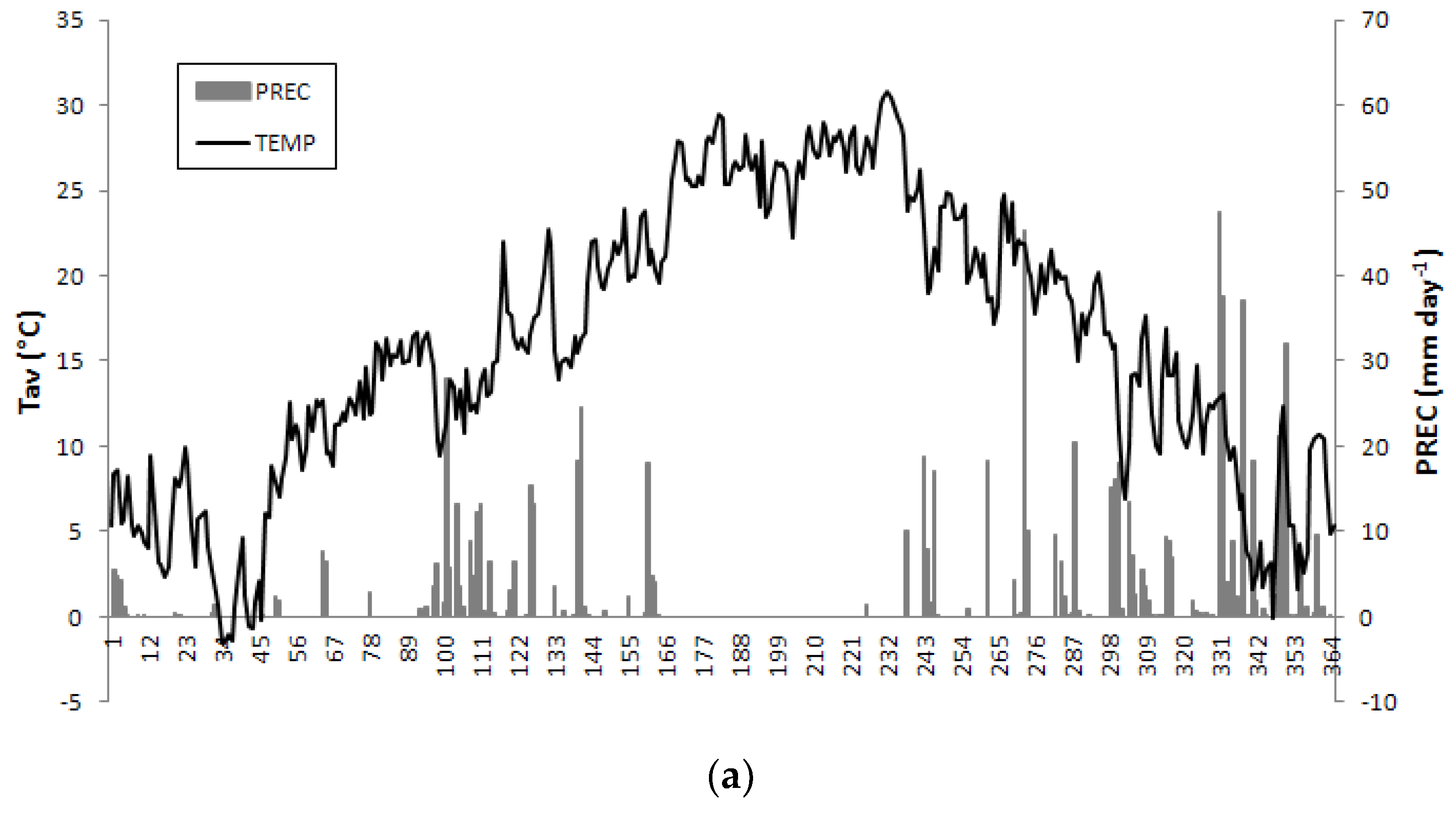
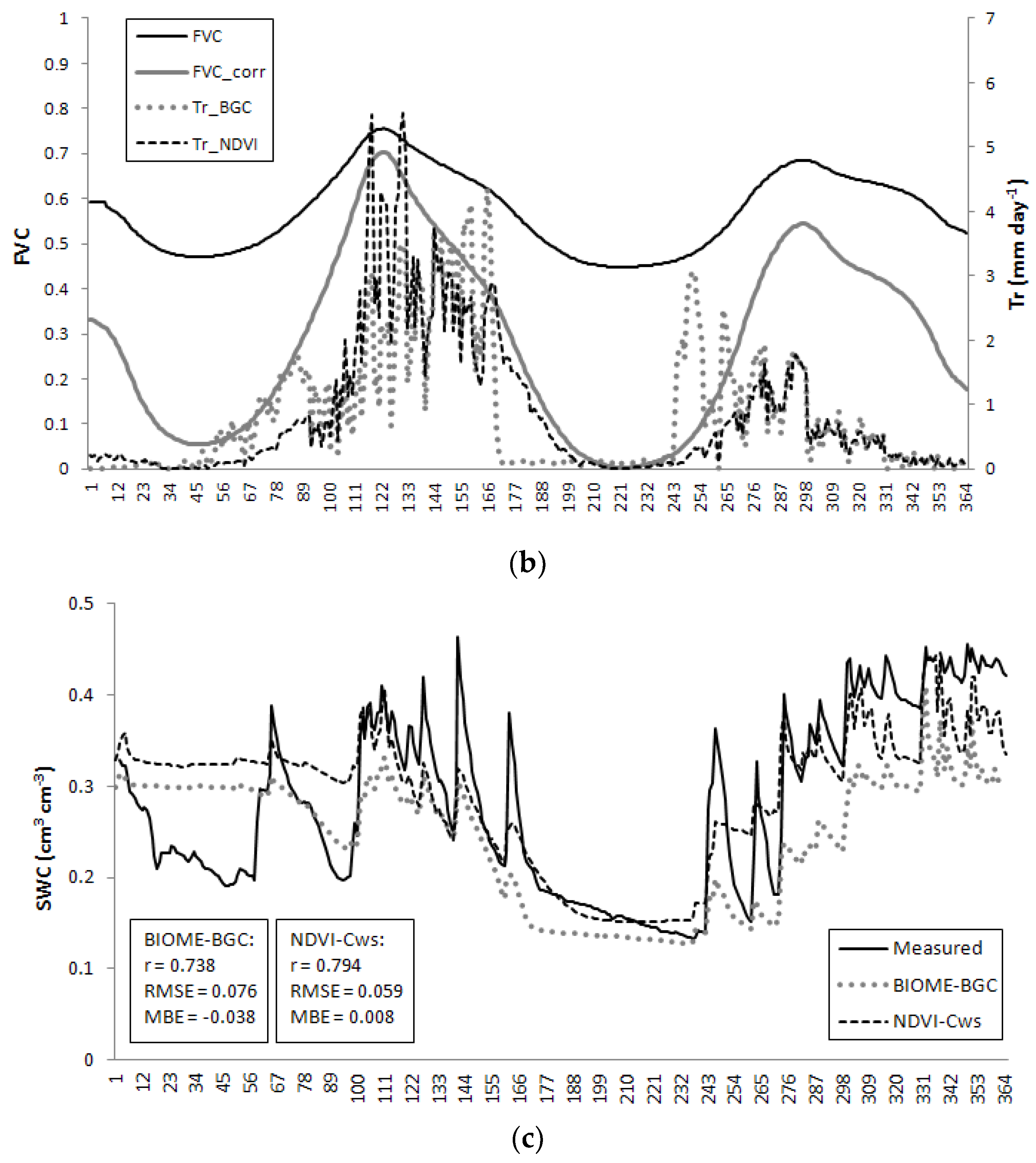
  • Amiata (42.9344° N, 11.6251° E) is situated in the south of Tuscany. The area is dominated by the presence of an ancient volcano; the altitude of the test site is about 758 m. The mean annual rainfall is about 800 mm and mean temperature is 12.4 °C. Summer is characterized by water shortage which, however, is not marked due to the site elevation. The whole area is quite homogeneous (over 5 ha) and is dominated by a coniferous forest (mostly Pinus nigra Arnold), with the marginal presence of some deciduous species (Quercus pubescens, Q. cerris, Q. ilex, etc.). Soil has a depth to bedrock of 0.7 m deep, is dominated by silt, and has a field capacity around 0.39 cm3 cm−3 (Table 2) [18].
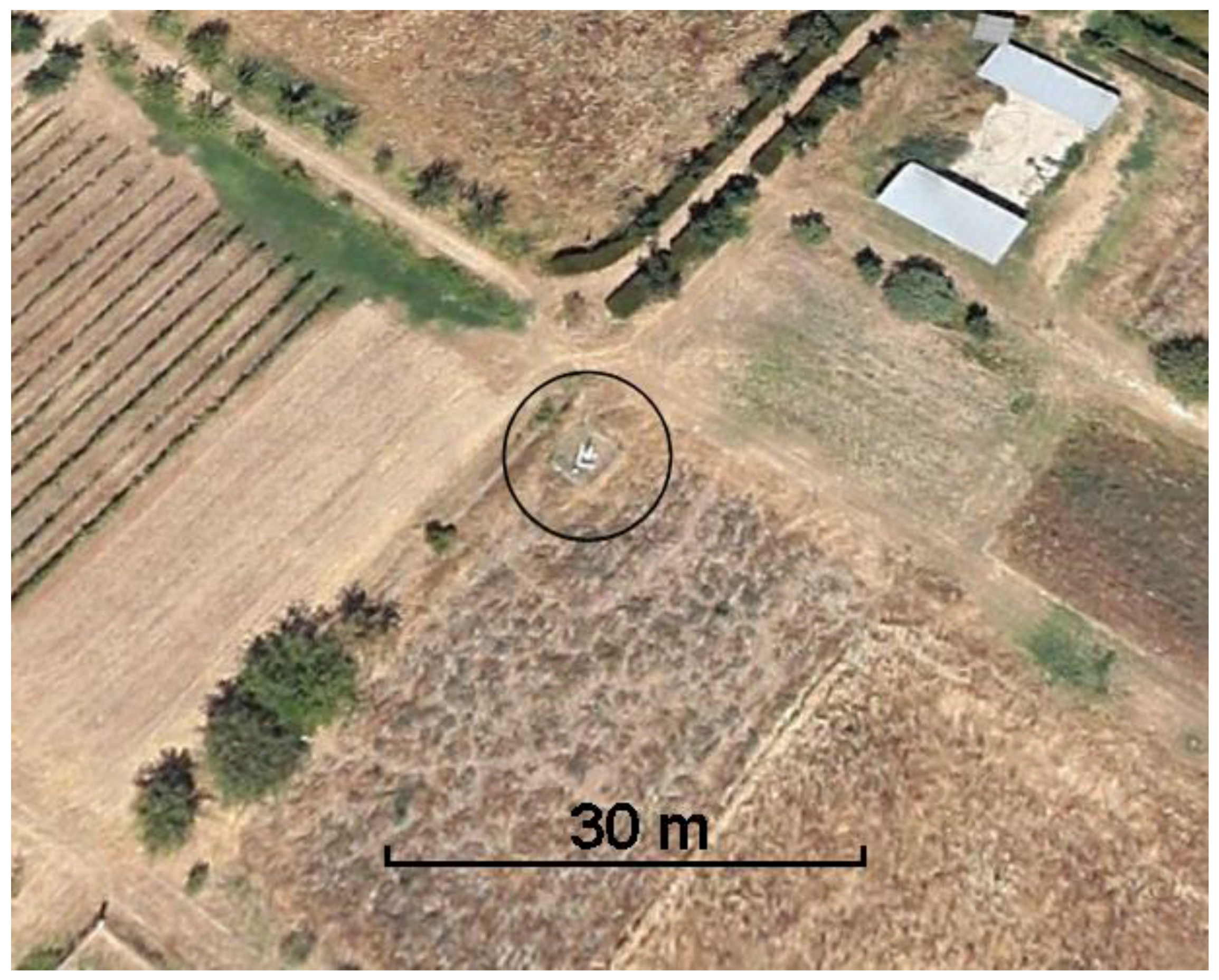
  • The third site is located within a small agricultural area close to the Urban Park of Cascine (43.7854° N, 11.2183° E) in Firenze. The area is flat, with an altitude of about 40 m. The annual rainfall is about 810 mm and the mean annual temperature 15.7 °C; rainfall is mostly distributed during autumn and spring, while summer is usually dry. The fields are small (below 0.2 ha) and mostly covered by grasslands and annual crops (mainly vegetables), surrounded by some vineyards and olive groves (Figure 2). The soil is sandy and very deep; no information is available on field capacity (Table 2).

2.2. Models Applied

2.2.1. BIOME-BGC

BIOME-BGC is a biogeochemical model able to estimate water, carbon and nitrogen storage, and fluxes of terrestrial ecosystems on a daily, monthly, or annual basis [7,20]. Among the inputs required for each simulation, there are site data (e.g., latitude, altitude, soil texture, and depth), daily meteorological data (e.g., maximum and minimum air temperature, precipitation, solar radiation), and ecophysiological parameters describing the behavior of vegetation growing over the area for which the simulation is performed.
All ecosystem processes are reproduced assuming that vegetation is represented by a unique layer, whose dimension is proportional to leaf area index (big-leaf approach). The hydrological cycle is simulated using a simple one-dimensional bucket model which does not include movements of water in deep soil layers and is constrained by the rooting depth (i.e., the depth at which plants are able to grow roots). This model considers precipitation (both rainfall and melted snow) as input to the soil, while the outputs are transpiration, soil evaporation, and outflow due to water exceeding field capacity. Thus, SWC at day i is computed as:
SWCi = SWCi−1 + Pi − ETAi − Oi
where Pi is precipitation, ETAi is evapotranspiration (i.e., soil evaporation plus transpiration), and Oi is outflow (i.e., percolation plus runoff), all referred to day i. The model version used (4.2) is the most recent one released by the Numerical Terradynamic Simulation Group (see http://www.ntsg.umt.edu/project/biome-bgc.php). Further details on the model functioning and calibration in the study region can be found in [7,21], respectively.

2.2.2. NDVI-Cws Method to Simulate SWC

NDVI-Cws is a recently proposed method which estimates the daily ETA of terrestrial ecosystems by the integration of ground and remotely sensed data [15]. This method utilizes satellite NDVI data to estimate the fractional vegetation cover (FVC), which indicates the quantity of green transpiring biomass that depends on long-term water stress. The estimation of FVC allows the separate simulation of plant transpiration and soil evaporation, which are limited by short-term water stress. The effect of this stress is accounted for by means of two meteorological factors, which are applied to vegetated and unvegetated cover fractions through the formula:
ETA = ET0i∙[FVC∙KcVeg∙Cws + (1-FVCi) ∙ KcSoil∙AW]
where KcVeg and KcSoil are maximum crop coefficient values (kc) of vegetation and soil, and Cws (coefficient of water stress) and AW (available water) are the two meteorological factors accounting for short-term water stress effect [15,22]. ETA is finally inserted into Equation (1), where all other terms are computed as in BIOME-BGC.

2.3. Data Utilized

Automatic SWC measurements were collected at each study site by means of capacitive probes (i.e., EC-5 TM for Barbialla and Amiata; Theta Probe ML2X for Cascine) situated at 0.2 m depth; hourly data were recorded and then aggregated on a daily basis. The data series covered different periods, that is, 2009–2012 for Barbialla, 2016–2017 for Amiata and 2008–2012 for Cascine.
For two of the study sites (Amiata and Cascine), daily meteorological data (minimum and maximum temperature and precipitation) were recorded at the SWC sampling area; for Barbialla, similar data were collected at the nearby ground stations of Peccioli for temperature and Fornacino for rainfall. Unfortunately, all these data sets were incomplete, which imposed the alternative use of data interpolated from nearby stations by the DAYMET algorithm [23]. This algorithm yielded a data set having a spatial resolution of 250 m for the period 1995–2016.
At each site, soil texture was determined by specific soil survey and sampling; the analytical determinations were carried out according to official methodologies [24]. The rooting depth was determined considering jointly the depth to bedrock and the ecosystem type (Table 2).
The land use map of the three study sites, which was necessary to analyze the low spatial resolution satellite images, was produced by visual interpretation of orthophotos acquired by aircraft flights in 2013; the photos were provided by the Tuscany Region Web Map Service (see http://www502.regione.toscana.it/geoscopio/servizi/wms/OFC.htm). Four land cover classes were identified (broadleaved and coniferous forests, grassland, urban areas), the first three of which were representative of the three ecosystem types considered. The influence of possible land cover changes was minimized by focusing all analyses on the year of SWC measurements closest to 2013, which was 2012 for Barbialla and Cascine and 2016 for Amiata.
MODIS NDVI images covering Central Italy were freely downloaded from the USGS database (http://lpdaac.usgs.gov; product MOD13Q1) for 2012 and 2016. These images have a 250 m spatial resolution and were composited over a 16-day period (Figure 1). For the highly fragmented urban area of Cascine, additional higher spatial resolution images were also collected in order to characterize the vegetation cover during the observed year. Three Google Earth images were fortunately available for this year, taken on 27 March 2012, 5 August 2012, and 19 October 2012; an example of these images, corresponding to the August acquisition, is shown in Figure 2.

2.4. Data Processing

The interpolated daily meteorological data were preliminarily checked against the corresponding data collected for each site during the respective test year. No significant difference between measured and interpolated data was observed (all relative errors were around 1–2%, data not shown). Daily solar radiation was therefore estimated applying the MT-CLIM algorithm to the interpolated data [25]. This data set, together with soil depth and texture available for each site, was utilized to drive BIOME-BGC and estimate SWC for the respective study years. The ecophysiological parameters for Barbialla, Amiata, and Cascine are equal to those proposed in previous literature [26,27], referring to plain/hilly conifers, deciduous oaks, and C3 grasses, respectively.
The same meteorological data were then used to predict daily ET0 by the empirical formula of [28]. The multitemporal NDVI profiles of the three vegetation classes considered (deciduous and coniferous forests and grassland) were extracted from the MODIS NDVI images of the study years by the method described in [29]. This method is capable of integrating the land cover map of each site with relevant MODIS images to identify the NDVI values of specific land cover units having an area over 1 ha. The 23 NDVI values found for the three vegetation types were then interpolated on daily basis and transformed into FVC by the linear equation proposed by [30] and calibrated by [15]. The mentioned spatial resolution was sufficient for the relatively homogeneous forest sites, while this was not the case for Cascine, which was characterized by high spatial heterogeneity (see Figure 2). Consequently, the FVC estimates of this site were recalibrated using the three higher spatial resolution Google Earth images available for 2012. The annual minimum and maximum FVC needed for this operation were determined by drawing on these images a small plot around the measurement site. The size of this plot (5 × 5 m) was defined considering the area which is actually influential on the SWC probe [31]. The plot was divided into 1 m2 quadrats, which were visually attributed to vegetated or bare soil for the three considered dates. The minimum and maximum FVC thus identified in March and August were finally used to linearly rescale the MODIS multitemporal profile, assuming that these periods coincided with the respective extremes of grassland cover.
In all cases, the FVC estimates were combined with the available meteorological data to predict daily ETA and SWC by Equations (1) and (2), respectively. The pedotransfer function proposed for Mediterranean areas by [19] was applied to the site soil textures for computing the respective field capacities. The daily SWC estimates produced by both models were finally checked against the available ground measurements. The results of the comparison were summarized using common accuracy statistics (i.e., correlation coefficient, r; root-mean-squared error, RMSE; mean bias error, MBE).

3. Results

3.1. Barbialla Site

The daily evolution of mean air temperature and precipitation at Barbialla during 2012 is shown in Figure 3a. The annual precipitation is about 900 mm and is distributed with three maxima (i.e., in April, September, and December) and a minimum during summer. Summer is also characterized by mean air temperature close to 30 °C, leading to a prolonged dry season from the beginning of June to the end of August.
This seasonal evolution affects FVC (Figure 3b), which shows two peaks (mid-May and early October) and a slight reduction in summer, attributable to the prevalence of deciduous trees and to the occurrence of summer water shortage. The transpiration estimates of BIOME-BGC are around 330 mm year−1; the seasonal evolution is only partly related to that of FVC, being characterized by a peak at the beginning of July, followed by a drop due to water scarcity. The NDVI-Cws transpiration estimates obviously follow more closely FVC, and the total amount of transpired water predicted by this method is about 480 mm.
The corresponding SWC measurements are shown in Figure 3c, together with the two simulated profiles. The measured field capacity is around 0.32 cm3 cm−3 and is not well reproduced by BIOME-BGC, which estimates a value around 0.25 cm3 cm−3 (Table 2). As a consequence, this model strongly underestimates SWC for the whole year. This problem is mostly corrected using the ETA estimates of the NDVI-Cws method and the field capacity predicted by the M4 model (0.30 cm3 cm−3). The strong SWC reduction due to summer dryness is evident in both measured and simulated profiles, but the former has an initial, abrupt decrease (from late May to the end of June) followed by a slighter reduction until the end of August, while the last two proceed more or less in parallel. The first rainy events at the end of August until early September are sufficient to increase SWC; the two simulation approaches, however, reproduce a lower soil water recharge. Globally, the accordance between measurements and estimates are good (more than 61% of variance is explained by both models), but the model which uses satellite data shows slightly lower errors both in terms of RMSE and MBE.

3.2. Amiata Site

At the Amiata site, during 2016, mean air temperature is never higher than 25 °C and summer is characterized by relatively warm days (drops below 15 °C) due to the occurrence of rainy events (Figure 4a). Rainfall is well distributed during the whole year, with maxima in winter and in autumn; the total amount of precipitation (1255 mm year−1) is higher than ET0 (872 mm year−1), indicating that water is not a major limiting factor for vegetation growth.
The seasonal weather evolution has an evident effect on the FVC profile of the pinewood (Figure 4b), which is nearly stable during the whole year due to the evergreen habitus of the trees, with only minor variations (between 0.7 and 0.9). The slightly lower values at the beginning of the year are presumably due to the deciduous component of the ecosystem (i.e., the understory or the sparse broadleaved trees). The two evolutions of simulated transpiration are quite similar during the whole year, with the exception of a difference in summer, when the NDVI-Cws method reaches higher daily values than the biogeochemical one (4.4 vs. 2.8 mm day−1) (Figure 4b).
The measured SWC data series, which is shown in Figure 4c, is atypical, being constantly lower than the measured field capacity (0.39 cm3 cm−3): the annual evolution is also rather irregular, mostly due to the occurrence of rainy events (see also Figure 4a). It mostly varies within 0.20 and 0.35 cm3 cm−3, with the exception of two peaks up to 0.45 cm3 cm−3 at the beginning of the year: these days correspond to rainfall higher than 40 mm day−1 in the second-half of February. The annual SWC variations are reproduced fairly well by both the biogeochemical model and the satellite-based simulation approach. Both approaches, however, overestimate the annual SWC evolution, with slightly lower error for the second method (MBE = 0.047 vs. 0.053 cm3 cm−3).

3.3. Cascine Site

For the Cascine site during 2012, the total annual rainfall is about 800 mm (Figure 5a); two maxima characterize its seasonal evolution, one in spring and the other in late autumn. Water shortage is therefore occurring in the hottest months, from June to September.
This pattern has important consequences on green biomass, which is notably reduced during late-spring and summer (Figure 5b). In this case, the FVC evolution is indicated by two lines. The first, which is directly derived from MODIS NDVI data, varies approximately between 0.45 and 0.70. These values do not agree with the FVC visually estimated from the Google Earth images, which ranges approximately between 0 and 0.7. As previously mentioned, these differences can be attributed to the low spatial resolution of MODIS data (250 m), which is not sufficient to characterize the small grass field containing the SWC probe, even when integrated with the available land cover map. The FVC recalibrated on the visually estimated values instead reproduces the expected pattern, showing variations which are typical of a dry Mediterranean grassland.
The difference between the transpiration profiles simulated by BIOME-BGC and the NDVI-Cws method fed with recalibrated FVC is particularly evident in this dry site. BIOME-BGC estimates reach the highest values in June and approach zero in summer, when no rainy days occur (see Figure 5a). The NDVI-Cws transpiration estimates show an earlier spring peak which is followed by a marked water stress period.
Measured and estimated SWC are shown in Figure 5c. All profiles are mostly concordant in reproducing the initial winter value, but the measurements show a reduction which is not captured well by the two modeling approaches. The dry period is concentrated around summer, followed by high water recharge at the beginning of September consequent on rainfall. BIOME-BGC is not capable of correctly reproducing the SWC reduction at the beginning of summer and the increase after fall rainfall. Concerning the satellite-based approach, the use of the original MODIS FVC produces a strong SWC overestimation (MBE = 0.189 cm3 cm−3; data not shown); this tendency is mostly corrected by using the recalibrated FVC, which yields good results both in terms of correlation and errors (r = 0.794; RMSE = 0.059 cm3 cm−3; and MBE = 0.008 cm3 cm−3).

4. Discussion

The analyses performed involved the use of several data sets and two simulation approaches, whose advantages and limitations are briefly reviewed in the following subsections.

4.1. Reference and Input Data Sets

Conventional field measurements of SWC provide observations which are intrinsically local in space, since the utilized probes are sensitive to small soil areas around them. The measurements are also affected by both systematic and random errors; the EC-5 sensors used in the current cases have an overall accuracy of ±0.03 cm3 cm−3 for most mineral soils [30,32]. Moreover, all SWC measurements were taken at 0.2 m depth and can hardly be considered representative of the soil layer corresponding to the actual plant rooting depth, which can be much higher (over 1 m). All these factors can give rise to uncertainty in the measurement of SWC, as is exemplified by the Amiata case, where the measured SWC profile seems not to fully match the field capacities determined by both laboratory analysis and the application of pedotransfer functions to soil texture observations.
The efficiency of the examined modeling approaches is obviously dependent on the quality of the input data sets used. Both approaches require daily meteorological data of the study period, but BIOME-BGC additionally needs long-term data sets to identify the quasi-equilibrium condition through the spin-up run [33]. The previously mentioned comparative analysis with the incomplete data sets taken at the site stations showed that the interpolated data currently used were quite accurate. Soil texture information is another fundamental input required to determine relevant hydraulic properties. The accuracy of this information was currently guaranteed by the collection and analysis of ground observations. The other fundamental driver, rooting depth, is functionally different from the depth to bedrock reported by usual soil maps, which prevents the direct use of the latter for the current modeling exercises. This problem was circumvented by defining the rooting depth taking into consideration both the soil depth and the ecosystem type. More sophisticated methods, however, can be envisaged, such as those proposed by [34].
The satellite images utilized for the NDVI-Cws method are freely available and can be easily processed to retrieve information on the fractional cover of green vegetation. This operation is relatively simple using MODIS imagery in spatially homogeneous areas, such as those surrounding the two study forest sites. The same operation is more problematic in cases of highly fragmented land cover, such as that of Cascine. In this situation, the use of higher resolution satellite images is essential to correctly detect the spatial variability of vegetation features. The integration of different satellite images has been currently performed using a very simple approach based on the visual analysis of very high resolution images, but more advanced techniques are available that can produce fused data sets with enhanced spatial and temporal features (e.g., [35,36]).

4.2. BIOME-BGC

Biogeochemical models are specifically suited to simulate the main fluxes through terrestrial ecosystems at a variety of spatial and temporal scales. Among these models, BIOME-BGC is very popular due to its easy applicability to different environments. This model, however, is crucially dependent on the proper setting of several ecophysiological parameters, which are difficult to define when dealing with specific biome types [20]. The settings currently used were specifically identified for Mediterranean ecosystems within previous investigations which particularly focused on the parameters related to the regulation of water losses (e.g., stomata conductance and leaf water potential, e.g., [21,26]).
The model capability to simulate ecosystem fluxes in different environments requires an oversimplification and generalization of some processes, which may be not always optimal. This is the case of the above-mentioned single-layer bucket approach, which considers outflow only when soil water exceeds field capacity and no movement of water between adjacent soil layers [37]. This approach is clearly suboptimal to estimate the SWC at the specific depth, which is measured by the ground sensors [38]. Some authors tried to modify this hydrological scheme by including flooding and the existence of a ground water flux [39], or adding a multilayer module (e.g., [38]); this exercise led to identification of a more complex modeling framework, not adopted in the current work.
Improvements in the model performance might also derive from a better estimation of field capacity on the basis of soil texture, since the pedotransfer functions used by BIOME-BGC show variable accuracy. In the case of Barbialla, for example, the measured field capacity is much lower than the estimated value, leading to a global underestimation of the SWC (Table 2). Another problem highlighted by the current investigation is the model tendency to overestimate the effect of summer water stress, almost nullifying the predicted ETA in the driest Mediterranean conditions. This is evident in the case of Barbialla and, above all, Cascine, where the ETA simulated during the driest summer period is extremely low. Such patterns are in accordance with the results obtained by other authors, who observed similar model limitations in arid and semiarid areas [40,41].
More generally, several studies have shown that BIOME-BGC is not optimal for site-specific agrometeorological applications but finds its maximum utility for the large-scale simulation of vegetation processes both in current and expected conditions [42,43]. This is confirmed by our results, which show that the model is generally capable of predicting the time variability of SWC even when the absolute values are not estimated well.

4.3. NDVI-Based SWC Simulation Approach

The NDVI-Cws method was developed to estimate ETA of both natural and agricultural vegetation, usually achieving satisfactory results. More specifically, [15] demonstrated the applicability of NDVI-Cws in different Mediterranean ecosystems, from deciduous to coniferous forests and annual crops. The results obtained—validated versus independent ETA observations derived from eddy covariance flux towers—highlighted the importance of using NDVI multitemporal profiles representative of the observed vegetation types.
The same approach was tested in an olive grove in Central Italy to estimate both transpiration and SWC [12]. In that case, the behavior of an agroecosystem characterized by two layers (i.e., herbs and olive trees) was simulated, reaching an accuracy comparable to that currently obtained for the three study sites. As previously noted, these three sites are representative of different Mediterranean ecosystem types, which provides a strong support to the general validity of the modeling approach.
Similar to BIOME-BGC, the efficiency of the approach is dependent on the correct definition of soil hydraulic properties by the use of suitable pedotransfer functions. Thus, functions calibrated for Mediterranean ecosystems outperform those used by BIOME-BGC, which are of more general validity; the estimated field capacities of Barbialla and Amiata, in fact, are quite close to the measured values (Table 2).
Overall, the current study confirms that the model based on NDVI-Cws is capable of correctly estimating daily SWC of different ecosystems with an accuracy which is generally higher than the biogeochemical model. This is mostly due to the use of the remotely sensed vegetation index, which is directly related to the amount of green transpiring biomass, an important contributor to site water balance and SWC in arid and semiarid regions [44]. The performances of the method are therefore strictly dependent on the capability of the remotely sensed NDVI data to correctly reproduce the spatiotemporal evolution of the existing vegetation.

5. Conclusions

The current study focused on the use of two modeling approaches for simulating the site water balance of three Mediterranean ecosystems which cover a gradient of aridity conditions and show different strategies in response to summer water stress. Tree species that characterize the Amiata and Barbialla sites show a greater control on water dynamics due to their higher total resistance to water loss, which allows the persistence of green leaf biomass during the dry summer period [45]. This is less the case for the grass of the Cascine site, which exhibits a water-spending strategy implying a notable reduction of green biomass during the driest summer periods [46].
The results obtained indicate that both modeling approaches are capable of reproducing the water dynamics in all these cases when fed with high-quality input data sets. In particular, BIOME-BGC can track the temporal variability of SWC but can only approximate the absolute SWC values due to the assumptions used (i.e., the one-layer bucket approach) and to its sensitivity to the parameter settings defining soil and vegetation features. Moreover, this biogeochemical model tends to overestimate the effect of summer water stress, excessively reducing the predicted ETA in the driest Mediterranean conditions.
These problems are mostly overcome by driving a similarly simplified bucket approach with ETA estimated by the integration of ground and remotely sensed data. The NDVI-Cws method, in particular, accounts for both long- and short-term effects of water stress, thus correctly simulating water loss through vegetation during the most critical periods. This property is dependent on the accurate estimation of the seasonal evolution of vegetation activity through FVC, which can require the proper integration of remote sensing data sets with different spatial and temporal properties. This requirement is particularly strict in Mediterranean areas, where vegetation types showing multiple growing cycles and water spending strategies are distributed in spatially fragmented and heterogeneous landscapes [35].

Author Contributions

P.B. and F.M. conceived and designed the experiments; M.C. B.R. and M.R., performed the experiments; F.S., E.S. and C.P. collected the ground data; S.R., L.F. and L.G. analyzed the data; M.C. and F.M. wrote the paper.

Acknowledgments

The following projects are thanked: (1) SELPIBIO LIFE Biodiversità (LIFE13 BIO/IT/000282), funded by EU and coordinated by CREA, for the collection of soil and meteorological data at Amiata; (2) MAGNATUM (Monitoraggio delle Attività di Gestione delle tartufaie Naturali di Tuber Magnatum), for funding soil sampling and analysis at Barbialla; (3) IMUCLIMA (Valutazione dell’impatto dei mutamenti climatici sulla produzione di tartufo bianco pregiato (Tuber magnatum Pico) nell’area delle colline sanminiatesi (Toscana-Italia) University of Siena), for funding the soil moisture monitoring at Barbialla. The authors wish to thank Dr. L. Angeli for pre-processing MODIS images and the four anonymous reviewers for their helpful comments on the first draft of the manuscript.

Conflicts of Interest

The authors declare no conflict of interest.

References

  1. Anderson, R.G.; Jin, Y.; Goulden, M.L. Assessing regional evapotranspiration and water balance across a Mediterranean montane climate gradient. Agric. For. Meteorol. 2012, 166–167, 10–22. [Google Scholar] [CrossRef]
  2. Milano, M.; Ruelland, D.; Fernandez, S.; Dezetter, A.; Fabre, J.; Servat, E.; Fritsch, J.-M.; Ardoin-Bardin, S.; Thivet, G. Current state of Mediterranean water resources and future trends under climatic and anthropogenic changes. Hydrol. Sci. J. 2013, 58, 498–518. [Google Scholar] [CrossRef]
  3. Bittelli, M. Measuring soil water content: A review. HortTechnology 2011, 21, 293–300. [Google Scholar]
  4. Devi, G.K.; Ganasri, B.P.; Dwarakish, G.S. A review on hydrological models. Aquat. Procedia 2015, 4, 1001–1007. [Google Scholar] [CrossRef]
  5. Waring, H.R.; Running, S.W. Forest Ecosystems, Analysis at Multiples Scales, 3rd ed.; Academic Press: San Diego, CA, USA, 2007. [Google Scholar]
  6. Bellot, J.; Chirino, E. Hydrobal: An eco-hydrological modelling approach for assessing water balances in different vegetation types in semi-arid areas. Ecol. Model. 2013, 266, 30–41. [Google Scholar] [CrossRef]
  7. Thornton, P.E.; Law, B.E.; Gholz, H.L.; Clark, K.L.; Falge, E.; Ellsworth, D.S.; Goldstein, A.H.; Monson, R.K.; Hollinger, D.; Falk, M.; et al. Modeling and measuring the effects of disturbance history and climate on carbon and water budgets in evergreen needleleafs forests. Agric. For. Meteorol. 2002, 113, 185–222. [Google Scholar] [CrossRef]
  8. Macelloni, G.; Paloscia, S.; Pampaloni, P.; Ruisi, R.; Dechambre, M.; Valentin, R.; Chanzy, A.; Wigneron, J.P. Active and passive microwave measurements for the characterization of soils and crops. Agronomie 2002, 22, 581–586. [Google Scholar] [CrossRef]
  9. Wang, L.L. Satellite remote sensing applications for surface soil moisture monitoring: A review. Front. Earth Sci. 2009, 3, 237–247. [Google Scholar] [CrossRef]
  10. Colliander, A.; Jackson, T.J.; Bindlish, R.; Chan, S.; Das, N.; Kim, S.B.; Cosh, M.H.; Dunbar, R.S.; Dang, L.; Pashaian, L.; et al. Validation of SMAP surface soil moisture products with core validation sites. Remote Sens. Environ. 2017, 191, 215–231. [Google Scholar] [CrossRef]
  11. Moreno, A.; Gilabert, M.A.; Camacho, F.; Martínez, B. Validation of daily global solar irradiation images 667 from MSG over Spain. Renew. Energy 2013, 60, 332–342. [Google Scholar] [CrossRef]
  12. Battista, P.; Chiesi, M.; Rapi, B.; Romani, M.; Cantini, C.; Giovannelli, A.; Cocozza, C.; Tognetti, R.; Maselli, F. Integration of ground and multi-resolution satellite data for predicting the water balance of a Mediterranean two-layer agro-ecosystem. Remote Sens. 2016, 8, 731. [Google Scholar] [CrossRef]
  13. Allen, R.G.; Pereira, L.S.; Raes, D.; Smith, M. Crop Evapotranspiration—Guidelines for Computing Crop Water Requirements—FAO Irrigation and Drainage Paper 56; FAO—Food and Agriculture Organization of the United Nations: Rome, Italy, 1998; 300p. [Google Scholar]
  14. Glenn, E.P.; Nagler, P.L.; Huete, A.R. Vegetation index methods for estimating evapotranspiration by remote sensing. Surv. Geophys. 2010, 31, 531–555. [Google Scholar] [CrossRef]
  15. Maselli, F.; Chiesi, L.; Angeli, L.; Papale, D.; Seufert, G. Operational monitoring of daily evapotranspiration by the combination of MODIS NDVI and ground meteorological data: Application and evaluation in Central Italy. Remote Sens. Environ. 2014, 152, 279–290. [Google Scholar] [CrossRef]
  16. Salerni, E.; Iotti, M.; Leonardi, P.; Gardin, L.; D’Aguanno, M.; Perini, C.; Pacioni, P.; Zambonelli, A. Effects of soil tillage on Tuber magnatum development in natural truffières. Mycorrhiza 2013. [Google Scholar] [CrossRef] [PubMed]
  17. Gardin, L.; Battista, P.; Bottai, L.; Chiesi, M.; Fibbi, L.; Rapi, B.; Romani, M.; Gozzini, B.; Maselli, F. Improved simulation of soil water content by the combination of ground and remote sensing data. Eur. J. Remote Sens. 2014, 47, 739–751. [Google Scholar] [CrossRef]
  18. Gardin, L. I Caratteri dei Suoli delle Aree Campione del Progetto SELPIBIO-LIFE; Technical Report; SOILDATA srl, Firenze; February 2018. [Google Scholar] [CrossRef]
  19. Jabloun, M.; Sahli, A. Development and comparative analysis of pedotransfer functions for predicting soil water characteristic content for Tunisian soil. In Proceedings of the 7th Edition of TJASSST 2006, Sousse, Tunisia, 4–6 December 2006; pp. 170–178. [Google Scholar]
  20. White, M.A.; Thornton, P.E.; Running, S.W.; Nemani, R.R. Parameterisation and sensitivity analysis of the BIOME-BGC terrestrial ecosystem model: Net primary production controls. Earth Interact. 2000, 4, 1–85. [Google Scholar] [CrossRef]
  21. Chiesi, M.; Maselli, F.; Moriondo, M.; Fibbi, L.; Bindi, M.; Running, S.W. Application of BIOME-BGC to simulate Mediterranean forest processes. Ecol. Model. 2007, 206, 179–190. [Google Scholar] [CrossRef]
  22. Maselli, F.; Papale, D.; Puletti, N.; Chirici, G.; Corona, P. Combining remote sensing and ancillary data to monitor the gross productivity of water-limited forest ecosystems. Remote Sens. Environ. 2009, 113, 657–667. [Google Scholar] [CrossRef] [Green Version]
  23. Thornton, P.E.; Running, S.W.; White, M.A. Generating surfaces of daily meteorological variables over large regions of complex terrain. J. Hydrol. 1997, 190, 214–251. [Google Scholar] [CrossRef]
  24. Italian Ministry for Agricultural and Forestry Politics (MiPAF). Official Methods of Soil Chemical Analysis; Gazzetta Ufficiale Supplemento Ordinario 248; Istituto Poligrafico e Zecca dello Stato: Rome, Italy, 1999. [Google Scholar]
  25. Thornton, P.E.; Hasenauer, H.; White, M.A. Simultaneous estimation of daily solar radiation and humidity from observed temperature and precipitation: An application over complex terrain in Austria. Agric. For. Meteorol. 2000, 104, 255–271. [Google Scholar] [CrossRef]
  26. Maselli, F.; Argenti, G.; Chiesi, M.; Angeli, L.; Papale, D. Simulation of grassland production by the combination of ground and satellite data. Agric. Ecosyst. Environ. 2013, 165, 163–172. [Google Scholar] [CrossRef]
  27. Chirici, G.; Chiesi, M.; Corona, P.; Salvati, R.; Papale, D.; Fibbi, L.; Sirca, C.; Spano, D.; Duce, P.; Marras, S.; et al. Estimating daily forest carbon fluxes using the combination of ground and remotely sensed data. J. Geophys. Res. Biogeosci. 2016, 121, 266–279. [Google Scholar] [CrossRef]
  28. Jensen, M.E.; Haise, H.R. Estimating evapotranspiration from solar radiation. J. Irrig. Drain. Div. ASCE 1963, 89, 15–41. [Google Scholar]
  29. Maselli, F. Definition of spatially variable spectral end-members by locally calibrated multivariate regression analyses. Remote Sens. Environ. 2001, 75, 29–38. [Google Scholar] [CrossRef]
  30. Gutman, G.; Ignatov, A. The derivation of the green vegetation fraction from NOAA/AVHRR data for use in numerical weather prediction models. Int. J. Remote Sens. 1998, 19, 1533–1543. [Google Scholar] [CrossRef]
  31. Kodešová, R.; Kodeš, V.; Mráz, A. Comparison of two sensors ECH2O EC-5 and SM200 for measuring soil water content. Soil Water Res. 2011, 6, 102–110. [Google Scholar] [CrossRef]
  32. Pardossi, A.; Incrocci, L.; Incrocci, G.; Malorgio, F.; Battista, P.; Bacci, L.; Rapi, B.; Marzialetti, P.; Hemming, J.; Balendonck, J. Root zone sensors for irrigation management in intensive agriculture. Sensors 2009, 9, 2809–2835. [Google Scholar] [CrossRef] [PubMed]
  33. Thornton, P.E.; Rosenbloom, N.A. Ecosystem model spin-up: Estimating steady state conditions in a coupled terrestrial carbon and nitrogen cycle model. Ecol. Model. 2005, 189, 25–48. [Google Scholar] [CrossRef]
  34. Sanchez-Ruiz, S.; Chiesi, M.; Fibbi, L.; Carrara, A.; Maselli, F.; Gilabert, M.A. Optimized application of BIOME-BGC for modeling of daily ecosystem gross carbon uptake over peninsular Spain. J. Geophys. Res. Biogeosci. 2018, 123. [Google Scholar] [CrossRef]
  35. Chen, B.; Huang, B.; Xu, B. Comparison of spatiotemporal fusion models: A review. Remote Sens. 2015, 7, 1798–1835. [Google Scholar] [CrossRef]
  36. Maselli, F.; Chiesi, M.; Pieri, M. A novel method to produce NDVI image series with enhanced spatial properties. Eur. J. Remote Sens. 2016, 49, 171–184. [Google Scholar] [CrossRef]
  37. Kimball, J.S.; White, M.A.; Running, S.W. BIOME-BGC simulations of stand hydrologic processes for BOREAS. J. Geophys. Res. 1987, 102, 29043–29051. [Google Scholar] [CrossRef]
  38. Hidy, D.; Barcza, Z.; Marjanović, H.; Sever, M.Z.O.; Dobor, L.; Gelybó, G.; Fodor, N.; Pintér, K.; Churkina, G.; Running, S.W.; et al. Terrestrial ecosystem process model Biome-BGCMuSo v4.0: Summary of improvements and new modeling possibilities. Geosci. Model Dev. 2016, 9, 4405–4437. [Google Scholar] [CrossRef]
  39. Pietsch, S.A.; Hasenauer, H.; Kucera, J.; Cermak, J. Modeling effects of hydrological changes on the carbon and nitrogen balance of oak in floodplains. Tree Physiol. 2003, 23, 735–746. [Google Scholar] [CrossRef] [PubMed]
  40. Mitchell, S.; Beven, K.; Freer, J.; Law, B. Processes influencing model-data mismatch in drought-stressed, fire-disturbed eddy flux sites. J. Geophys. Res. 2011, 116, G02008. [Google Scholar] [CrossRef]
  41. González-Sanchis, M.; Del Campo, A.D.; Molina, A.J.; Fernandes, T.J.G. Modeling adaptive forest management of a semi-arid Mediterranean Aleppo pine plantation. Ecol. Model. 2015, 308, 34–44. [Google Scholar] [CrossRef]
  42. Tatarinov, F.A.; Cienciala, E. Long-term simulation of the effect of climate changes on the growth of main Central-European forest tree species. Ecol. Model. 2009, 220, 3081–3088. [Google Scholar] [CrossRef]
  43. Fibbi, L.; Chiesi, M.; Moriondo, M.; Bindi, M.; Maselli, F. Analysis and simulation of climate impacts on the GPP of Mediterranean forests. Clim. Chang. in revision.
  44. Gu, D.; Wang, Q.; Otieno, D. Canopy Transpiration and Stomatal Responses to Prolonged Drought by a Dominant Desert Species in Central Asia. Water 2017, 9, 404. [Google Scholar] [CrossRef]
  45. Pereira, J.S.; Mateus, J.A.; Aires, L.M.; Pita, G.; Pio, C.; David, J.S.; Andrade, V.; Banza, J.; David, T.S.; Paco, T.A.; et al. Net ecosystem carbon exchange in three contrasting Mediterranean ecosystems—The effect of drought. Biogeosciences 2007, 4, 791–802. [Google Scholar] [CrossRef]
  46. Hidy, D.; Barcza, Z.; Haszpra, L.; Churkina, G.; Pinter, K.; Nagy, Z. Development of the Biome-BGC model for simulation of managed herbaceous ecosystems. Ecol. Model. 2012, 226, 99–119. [Google Scholar] [CrossRef]
Figure 1. MODIS normalized difference vegetation index (NDVI) image of August 2013 showing the geographical position of the three study sites (Barbialla, Amiata, and Cascine) in Central Italy. The geographical window is 42–45° N, 8–13° E.
Water 10 00665 g001
Figure 2. Google Earth image taken on 5 August 2012 over the Cascine site. The black circle indicates the position of the weather station and soil water content (SWC) probe.
Water 10 00665 g002
Figure 3. (a) Daily mean air temperature and precipitation interpolated for the Barbialla site; (b) daily fractional vegetation cover (FVC) derived from NDVI and transpiration estimated by BIOME-BGC and NDVI-Cws; (c) daily SWC measured and estimated by the two modeling approaches. Errors are given in cm3 cm−3.
Water 10 00665 g003aWater 10 00665 g003b
Figure 4. (a) Daily mean air temperature and precipitation interpolated for the Amiata site; (b) daily FVC derived from NDVI and transpiration estimated by BIOME-BGC and NDVI-Cws; (c) daily SWC measured and estimated by the two modeling approaches. Errors are expressed in cm3 cm−3.
Water 10 00665 g004
Figure 5. (a) Daily mean air temperature and precipitation interpolated for the Cascine site; (b) daily FVC (original and corrected) derived from NDVI and transpiration estimated by BIOME-BGC and NDVI-Cws; (c) daily SWC measured and estimated by the two modeling approaches. Errors are expressed in cm3 cm−3.
Water 10 00665 g005aWater 10 00665 g005b
Table 1. Main ecoclimatic conditions of the three selected study sites. Climatic data are averaged over the period 1995–2016.
Study SiteAltitude (m)Mean Temperature (°C)Rainfall (mm)Ecosystem TypeData Availability
Barbialla13515.1810Mixed forest2012
Amiata75812.4850Coniferous forest2016
Cascine4015.7810Grassland2012
Table 2. Rooting depth and soil texture (expressed in g kg−1) derived from local samples for each study area; the last columns report soil water content at field capacity determined by laboratory analysis and estimated by BIOME-BGC and the M4 model proposed by [19] (see text for details).
Study SiteRooting Depth (m)SandSiltClayField Capacity (cm3 cm−3)
MeasuredBIOME-BGCM4 Model
Barbialla1.206.03.01.00.3200.2460.300
Amiata0.701.35.33.40.3900.4230.358
Cascine0.505.22.42.4-0.3010.328

