Observation of the Dynamics and Horizontal Dispersion in a Shallow Intermittently Closed and Open Lake and Lagoon (ICOLL)

Abstract

Among the 135 or more estuaries on the southeast Australian coastline, 45% are intermittently open. A number of others, which would normally have an intermittently open entrance, are kept permanently open to improve the flushing and water quality that are functions of the horizontal dispersion of the estuarine system. Field studies that investigate the dynamics and horizontal dispersion processes of open and closed states of Intermittenly Closed and Open Lakes and Lagoons (ICOLL) are conducted. Clusters of Lagrangian drifters were used to characterise the surface flow. Horizontal dispersion coefficients (K) under study varied significantly for different tidal phases; the mean ebb tide K (~4.7 ± 3.8 m² s⁻¹) is an order of magnitude higher than that of the flood tide. During the closed state, K values were up to two orders of magnitude lower than those observed in the open state. These results highlight the contribution of tidal dispersion to transport and mixing processes within an ICOLL. The results showed that tidal pumping effects and tidal-induced horizontal velocity gradients are responsible for the horizontal surface transport and dispersion occurring during the open inlet state. The horizontal surface dispersion processes identified at different inlets and environmental conditions within this site are valuable for managing transport of particles, freshwater mixing, larvae transport, waste, and pest control.

1. Introduction

Intermittently Closed and Open Lakes and Lagoons (ICOLLs) are a subcategory of coastal lakes and lagoons, which exhibit limited exchange with the ocean and river flows [1]. Of the more than 135 estuaries along the southeast Australian coast, about 45% of these are intermittently open and a number of others, which would normally have intermittently open entrances, are kept permanently open. The permanent open state is facilitated by mechanical means to maximize the flushing and water quality that are functions of the horizontal dispersion of the system [2,3]. Many prior studies on ICOLLs have focused on the change in ecological processes caused by their dynamic opening and closing [4,5]. Hydrodynamic processes including vertical mixing, and horizontal dispersion, flushing, and recirculation patterns control the ecological processes [6,7]. Previous research demonstrates the susceptibility of ICOLLs to periods of stratification during both closed and open states, which influences the concentration of dissolved oxygen (DO) [1,6]. These studies highlight that stratification is due to the combination of low wind, periods of rainfall, and high solar insolation in the closed state. In addition to these factors, open state stratification is governed by variations in tidal mixing processes. The result provides insight into how inlet conditions affect vertical mixing, and in turn DO (among other water quality parameters). Horizontal transport/mixing processes controls distribution of nutrients, sediment, and contaminants [8]. These processes and how they are affected by inlet conditions are, however, rarely studied from field observations due to significant logistical and financial constraints.

Measuring horizontal surface transport, and the spreading of passive scalars has wide practical applications including modeling of material (particles and solutes) transport and estimation of time-scales for removal of these materials [9]. In addition, examining the dispersion behavior informs estuary management when considered in conjunction with geomorphic characteristics, system eco-health, social dynamics, and asset risk profiles of the target catchment area, thus, providing better targeting of nutrient laden runoff, improved calibration and validation of models.

Dispersion is traditionally studied using dye or salinity tracer experiments where horizontal dispersion coefficients are estimated [10,11,12]. An alternative, less expensive approach, is to use flocks of GPS-tracked Lagrangian drifters [13]. This approach has recently been introduced in riverine and estuarine systems as the accuracy and resolution of GPS technology has improved [14,15,16]. The growth of a cluster of particles (such as larvae and buoyant pollutants) in the surface layer is governed by several mechanisms [17]. These include irreversible turbulent dispersion caused by fluctuations in the velocity field at scales smaller than the cluster size, horizontal shear dispersion caused by horizontal velocity gradients at scales larger than the cluster size, and small-scale horizontal flow fluctuation and vertical shear dispersion caused by small-scale vertical fluctuations [10,17,18]. A comprehensive understanding of horizontal in-channel dispersion requires individual quantification of each mechanism at a wide range of time scales.

Currimundi Lake is a coastal lagoon located on Queensland’s Sunshine Coast in Eastern Australia. The surrounding area has high recreational, environmental, social, and economic values. Management of this natural resource is complex, balancing dynamic stakeholder issues (e.g., those of residents, day visitors, tourism industry and governments) and the maintenance of a sustainable healthy estuarine system. The system is generally classified as an ICOLL. Like many coastal areas, biting midge at the peak breeding season is a major problem in Currimundi Lake [19]. While tidal cycles have been observed to aid breeding of intertidal biting midge species [19], recent research has shown that the larvae of many species are not able to survive inundation for a long period [20]. Therefore, Currimundi Lake is sometimes artificially disconnected from the ocean by blocking the inlet to raise the water level to manage the biting midge population by drowning midge larvae in the sand banks [21]. One of the main catchment management concerns is understanding the horizontal flow dynamics of the channel for the open and closed conditions and how this operation affects biting midges, litter distribution, physiochemical properties, and sediment transport. For managing these issues and other similar dispersion problems, a detailed spatio-temporal advection-dispersion model is necessary [9]. An important input to this model is the horizontal dispersion coefficient which represents the range of dominant mechanism in the channels at different times, particularly at scales less than a tidal cycle. Dispersion coefficient parametrized as a function of length scale (30 m–100 km) obtained from large water bodies might not be applicable to this shallow estuary due to difference in scale of processes (O [1 m]), particularly at time scales less than a tidal period [16,22].

As part of an on-going study to develop a robust model for addressing various management concerns in the Currimundi Lake ICOLL, a series of field studies are being carried out at various baseline inlet conditions [23]. Using the field data collected during the open and closed conditions, the objectives of the current contribution include: (i) estimate of dispersion coefficients using flocks of drifters, (ii) contrasting the dispersive properties of the channel during these inlets conditions, and (iii) identifying the dominant dispersion mechanism for the inlet conditions. The purpose of this article is to present estimates of dispersion coefficients and dominant dispersion mechanisms from field studies in an ICOLL that provide an insight into transport of material in the systems during open and closed conditions, for time scale less than a tidal cycle and length scale in the order O [1 m].

2. Materials and Methods

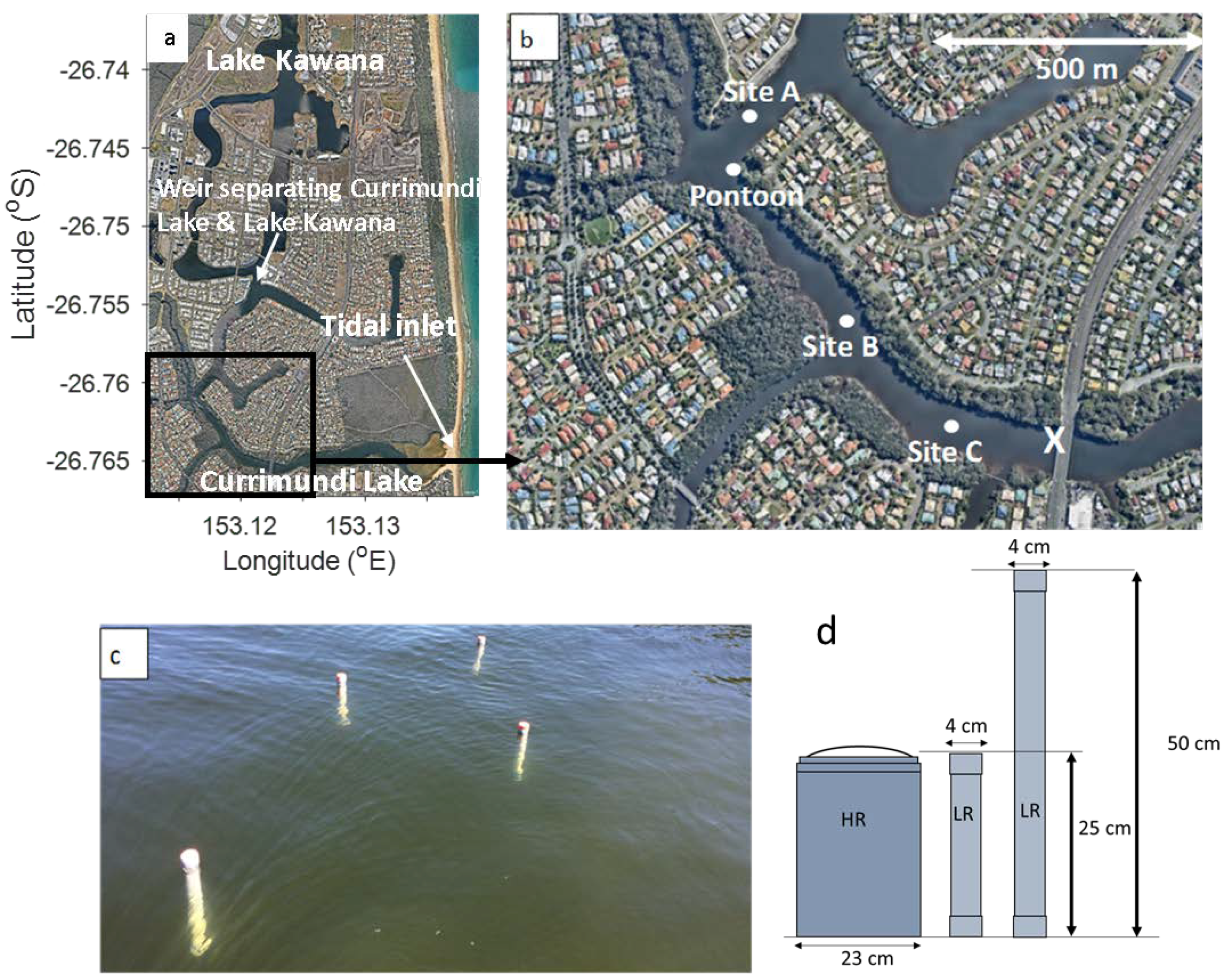
2.1. Study Area

Currimundi Lake (Longitude 153.13° E, Latitude 26.763° S) is a coastal lagoon located on Queensland’s Sunshine Coast in eastern Australia (Figure 1). The local climate is subtropical with an annual rainfall greater than 1200 mm with most rainfall (>60%), in the summer and part of autumn, between December and March. The location is characterized with average wind speeds between 5 m s⁻¹ from the NE-E direction in the second half of a year and 6.8 m s⁻¹ from the S-SE directions the first half of a year. The average daily global solar exposure is 5 kWh/m² (208.3 W/m²) with the lowest of 2.9 kWh/m² (121 W/m²) in June and highest of 7.6 kWh/m² (317 W/m²) in January [24]. The catchment area for Currimundi Lake is highly urbanised having experienced significant growth commencing around the 1950s. The lower main channel of Currimudi Lake is connected to the ocean and upstream links to a range of stormwater infrastructure, canal networks, and a constructed brackish water body (Lake Kawana). To ensure that water circulation and turnover rates within Lake Kawana are maintained, an exchange system draws freshwater from the Mooloolah River System through Lake Kawana, discharging into the Currimundi Lake system via a weir (Figure 1a) at an average rate of 80 mL/day when the mouth is open. During the closed state, the discharge rate varies between 0–80 mL/day depending on the need to supplement the lake water level inundation of biting midge breeding sites located within the intertidal areas.

The Currimundi Lake main channel is characterised by a mixed tide with a predominantly semi-diurnal tidal pattern and is a micro-tidal estuary with a spring tidal range limited to 0.8 m. The depth of the channel ranges between 3–5 m mid-estuary. The system is considered an ICOLL with the recorded natural opening and closing events prior to the current field experiments, in the early 2000s and was naturally closed recently in July 2017 [25]. However, from the mid-2000s it has been artificially disconnected from the ocean once per year, by blocking the inlet with sand, usually for about six weeks in September/October.

Three different drifter experiments were conducted along the main channel during tidal (open state—E1 in 27–28 April 2015) and non-tidal (closed state—E2 in 9 September 2015) conditions, and during the opening of the inlet (E3 in October 2015). Here we focus on the effect of the inlet condition on the dynamics and the horizontal surface dispersion of channel flow by contrasting observations during the open (E1) and closed state (E2) experiments. The forcing conditions for the two experiments are discussed in details in the next Section 2.2.

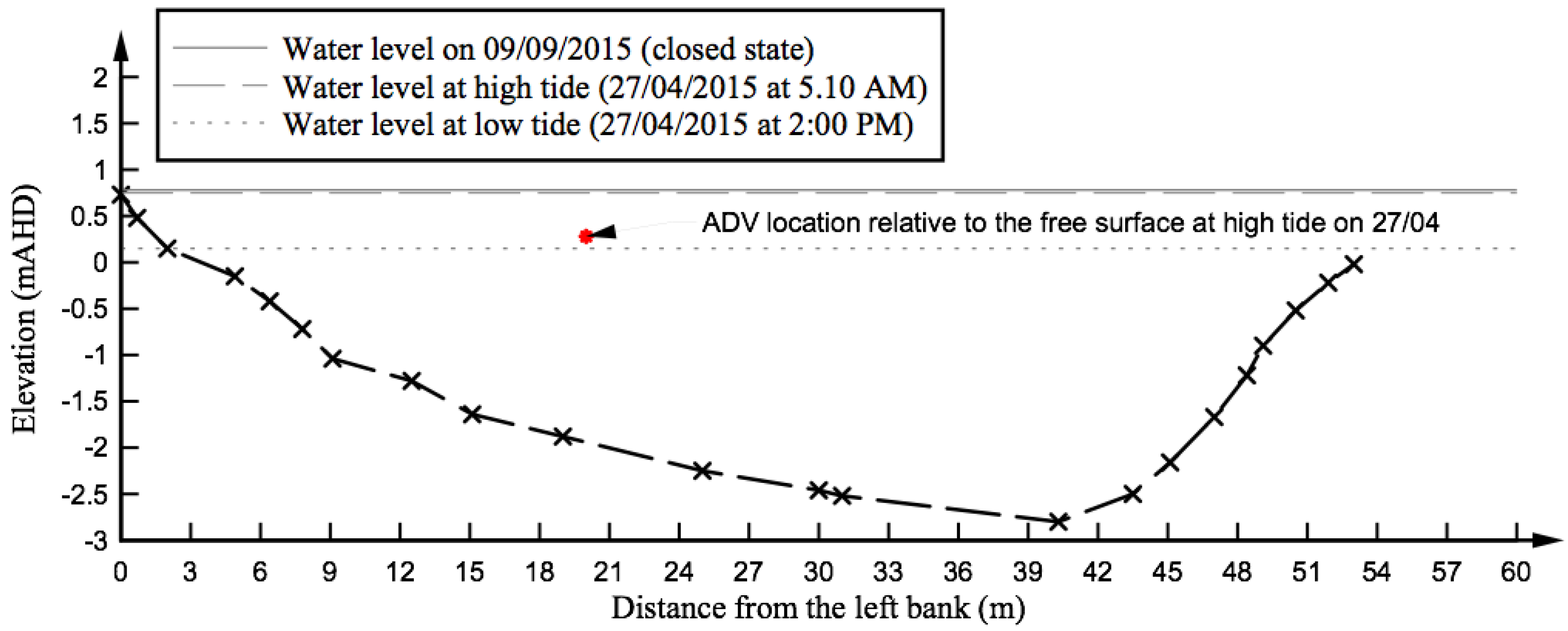
2.2. Environmental and Inlet Conditions during the Field Experiments

The major forcing conditions in Currimundi Lake during an open condition include tide, river discharge, wind and rainfall. In the absence of tidal forcing in a closed state, the solar radiation and heat convection potentially become important. A range of tide, wind, solar exposure and flow conditions was encountered during the field studies (

Table 1. Summary of the experimental conditions and instruments deployed at Currimundi Lake; flow velocity and wind speed were measured using ADV, weather station and sonic anemometer deployed at the Pontoon (Figure 1b).

Experiment	Date	Inlet Condition	Tide	Tidal Range (m)	Water Depth at X (m)	Daily Mean Solar Exposure (W/m2)	Wind Speed Range (m s−1)	Average Flow Velocity (m s−1)	Instrument Deployed
E1	27/4/15–28/4/15	Open	Flood	0.60	0.4–1.1	175	0–4.0	0.10	ADV and GPS-drifters, weather station
			Ebb		0.5–0.8			0.10
E2	09/09/15	Closed	Non-tidal	0.00	1.1	287.5	0–7.0	0.04	GPS-drifters, and Sonic anemometer

). During the open state (E1), the average tidal range was 0.6 m. The average fresh water input into the channel from Lake Kawana was 80 mL/day for the open state. During the closed state, the water level indicated a gradual increase of 0.1 m between 31 August 2015 and 2 September 2015, likely from the combination of storm water run-off and freshwater from Lake Kawana, and the water level then remained approximately constant at 0.78 m AHD through the closed state experiment (Figure 2c). The total rainfall within the catchment seven days prior to the measurements was less than 10 mm for both open and closed states. Therefore, runoff from storm water drains was assumed to be insignificant. The wind velocity peaked at 4 and 7 m s⁻¹ from the S-SE directions for the open and closed experiments, respectively.

Water level, salinity, and temperature of the channel are continuously monitored by the Sunshine Coast Council (SCC) at the bridge marked X in Figure 1b. The water level in the channel was between 0.08–0.78 m Australian Height Datum (m AHD) during the open state (E1), while the water level was constant at 0.78 m AHD during the closed state (E2) experiment (Figure 2). The water levels are shown relative to the surveyed bed profile near the pontoon in Figure 3. A Conductivity, Temperature and Depth meter, CTD3100, was used to sample water quality at a temporal resolution of 5 min placed at −0.32 m AHD elevation. Figure 2 shows the time series of water level and salinity during the open state (E1) and the closed state (E2) experiments. During the open state (E1), the water level and salinity exhibited tidal trends. The diurnal trend in the salinity observed during the closed state (E2) is likely associated with daily thermal and wind mixing in the water column.

2.3. Instrumentation

To examine the horizontal surface dispersion within the channel, Lagrangian drifters were deployed. The drifters used in this study are similar in shape and design, but different in dimension and electronic components to high resolution (HR) drifters described by [13]. These low cost, low resolution (LR) drifters are made of PVC cylindrical pipes with 4 cm diameters and lengths of 25 and 50 cm for the short and long types, respectively (Figure 1d). The drifters contain off-the-shelf Holux GPS data loggers with absolute position accuracy of 2–3 m, sampled at 1 Hz. The effect of this error on analysed parameters is discussed in Section 2.3. The drifters were positively buoyant for continuous satellite position fixation with <3 cm height unsubmerged to limit wind effects [13,26]. The current configuration results in direct wind slip estimated as less than 1% of the ambient wind for the short drifter version [13,26,27,28]. The drifters showed good agreement (R² ~ 0.9) with surface velocity measurements obtained from an Acoustic Doppler Current Profiler (ADCP) within a 60 m radius [26,29]. However, unfiltered drifter data are not suitable for measuring small-scale processes in low flow applications because of the inherent position error that manifests as a large speed variance; σ² ~ 0.0005 m² s⁻² in stationary tests at frequencies F > 0.01 Hz [23].

Although a Lagrangian drifter has been shown to be applicable to studying shallow water systems, there are clear limitations to its application to ICOLL due to stratification and ensuing baroclinic motions, particularly in closed states. The drifter used in the current study is designed to follow the upper 0.5 m layer of the water column; therefore, the observed dispersion coefficients and dynamics are representative of horizontal surface dispersion. In addition, the drifter only captures motion on a scale greater than its radius; therefore, the size limits the range of eddies it captures. Further limitations of drifter application to examining dispersion in shallow waters are discussed in [13].

During the open state (E1), a fleet containing 10 short and 10 long drifters was deployed in the ebb and flood tides on 27 April 2015. Eighteen drifters were retrieved at the end of the experiment; two drifters were lost. The ebb deployment occurred at Site A (Figure 1b), adjacent to the main channel, while the flood deployment was made at Site C, upstream of the bridge marked X. The drifters were deployed in a line abreast configuration with approximately 1 m separation [23]. Drifters trapped along banks were collected and redeployed at the adjacent centerline. Data quality control is described in Section 2.3. During the 4-h ebb tide experiment, the number of times an individual drifter reached the banks varied from two to nine with an average of six times per drifter. Conversely, only five of the 18 drifters were redeployed during the 3-h flood tide experiment. This suggests that the ebb surface current induced many recirculation zones close to the banks, trapping the drifters. During the closed state (E2), all deployments occurred at Site B. Drifters were deployed in four clusters (C1, C2, C3 & C4), each containing 3–5 drifters at the centre of the channel. Two separate deployments were made for each cluster during the 6-h field experiment. The drifters all moved upstream toward the pontoon (Figure 1), due to wind forcing.

A Sontek^® Acoustic Doppler Velocimeter (ADV) sampling at 50 Hz was mounted rigidly to the pontoon 0.5 m below the water surface to capture surface flow velocity. Figure 3 shows the profile of the transect next to the pontoon and the corresponding location of the ADV. Coinciding with the drifter experiments during the closed state (E2), vertical profiles of DO, salinity, and temperature were collected by the Sunshine Coast Council at the pontoon and the bridge (X) (Figure 1) using Hydrolab DS5X. In addition, a two-dimensional wind anemometer was mounted next to the pontoon about 0.5 m above the water surface to capture the wind speeds and directions at the free surface.

2.4. Data Analysis

Raw drifter data were converted to local East-North-Up (ENU) coordinates from a World Geodetic System (WGS84). The drifter position data were quality controlled using velocity and acceleration de-spiking [13]. Sections of the trajectories where the drifters did not float in the channel, where they were found next to the bank or affected by occasional proximity to boats were removed using MATLAB scripts developed to work with the experimental event log. A low-pass filter with cut off frequency, F_c = 0.01 Hz, was then applied to the position time series. Drifter velocities relative to East and North were obtained by combining the quality controlled position and speed time series, which are directly logged by holux data-loggers:

$$V_E(t)=Sp(t)\times \mathrm{c}os\theta (t), V_N(t)=Sp(t)\times \mathrm{s}in\theta (t), \mathrm{and} \theta (t)=\arctan \left(\frac{N(t)}{E(t)}\right),$$

(1)

where V_E and V_N are the Easting and Northing velocities, respectively, θ is the direction based on the position time series (E,N), and Sp is drifter speed at time t.

The objective of the cluster analysis herein was to estimate the time variation mean values of the dispersion coefficient (K_c) and differential kinematic properties (DKP) for individual drifter deployments. The dispersion coefficient was obtained using the method described by [30]. The key aspect of the method is the calculation of the rate of change of a patch size with the assumption that the drifters are ‘locked’ to the ‘patch’ of fluid within which they were deployed.

Cluster analysis only commenced once data from all drifters in the cluster are simultaneously logged. However, the initial 300 s of measurement, when drifter motion was affected by boat movement and initial deployment, was excluded. For the open state (E1), where drifters were frequently beached and re-introduced into the channel, times with drifter numbers n < 5 were noisy and were not included in the results; therefore, at least five drifters were used in the calculation. For the closed state (E2), calculations were terminated immediately when one drifter in a single cluster was beached. The dispersion coefficient (K_c) estimates for long and short drifter clusters were similar during most of the experiment. Therefore, both drifter types were combined into a single cluster to improve the stability of the estimate. Using the local ENU coordinates, the centroid (represented with overbar) of a cluster is defined as:

$$\overline{E}(t)=\frac{1}{n}{\displaystyle \sum _{i=1}^n{E}_i}(t), \overline{N}(t)=\frac{1}{n}{\displaystyle \sum _{i=1}^n{N}_i}(t),$$

(2)

where i is the drifter counter and n is the total number of active drifters in a cluster at time, t. The variance of an individual drifter from the centroid of the cluster is then defined as:

$${\sigma }_E^2(t)=\frac{1}{n-1}{\displaystyle \sum _{i=1}^n[E_i}(t)-\overline{E}(t){]}^2, {\sigma }_N^2(t)=\frac{1}{n-1}{\displaystyle \sum _{i=1}^n[N_i}(t)-\overline{N}(t){]}^2.$$

(3)

The cluster relative dispersion coefficient is calculated from the averaged variance such that:

$$K_C(t)=\frac{1}{2}\frac{\partial {\sigma }^2(t)}{\partial t}, \mathrm{where} {\sigma }^2(t)=\frac{1}{2}\left[{\sigma }_E^2(t)+{\sigma }_N^2(t)\right]$$

(4)

DKP values were calculated from velocity gradients obtained via a Taylor’s series expansion about the centre of mass of a cluster, following the method described in [31]. This method assumes that the fluid domain is small and finite in size, such that the velocity gradient is uniform across a cluster. Therefore, the calculations were not conducted when a member of a cluster was within close proximity of a bank where strong velocity gradients are expected. The method further assumes that cluster velocity is correctly represented in the linear (first order) term of a Taylor’s series, while the second and higher order terms are considered as turbulence. Individual drifter velocity can be described as:

$$\begin{gathered} V_E(t)={\overline{V}}_E(t)+\frac{\partial {\overline{V}}_E(t)}{\partial E}\left[E(t)-\overline{E}(t)\right]+\frac{\partial {\overline{V}}_E(t)}{\partial N}\left[N(t)-\overline{N}(t)\right]+v_E(t) \\ {V}_N(t)={\overline{V}}_N(t)+\frac{\partial {\overline{V}}_N(t)}{\partial E}\left[E(t)-\overline{E}(t)\right]+\frac{\partial {\overline{V}}_N(t)}{\partial N}\left[N(t)-\overline{N}(t)\right]+v_N(t) \end{gathered}$$

(5)

where $\frac{\partial {\overline{V}}_E}{\partial E}$, $\frac{\partial {\overline{V}}_E}{\partial N}$, $\frac{\partial {\overline{V}}_N}{\partial E}$ and $\frac{\partial {\overline{V}}_N}{\partial N}$ are linear centroid velocity gradient terms, and $v_N$ and $v_E$ are non-linear turbulence velocity terms (second and higher order terms). The velocity gradient and non-linear terms are estimated using a least squares approach which converts the equation into a matrix format [31]. The non-linear turbulence terms are not presented here because their magnitudes are not significantly higher than the standard deviation of the speed of the drifter placed in a fixed location (i.e., during a stationary test). DKPs were then described in terms of the resulting velocity gradients such that:

$$\begin{array}{l}\mathrm{Horizontal}\mathrm{divergence}\delta (t)=\frac{\partial {\overline{V}}_E(t)}{\partial E}+\frac{\partial {\overline{V}}_N(t)}{\partial N},\\ \mathrm{Vorticity}\zeta (t)=\frac{\partial {\overline{V}}_N(t)}{\partial E}-\frac{\partial {\overline{V}}_E(t)}{\partial N},\\ b(t)=\frac{\partial {\overline{V}}_N(t)}{\partial E}+\frac{\partial {\overline{V}}_E(t)}{\partial N},\\ \mathrm{Stretching}\mathrm{deformation}a(t)=\frac{\partial {\overline{V}}_E(t)}{\partial E}-\frac{\partial {\overline{V}}_N(t)}{\partial N}\end{array}$$

(6)

The horizontal divergence (δ) is a measure of change in area of the cluster without a change in orientation or shape, while relative vorticity (ζ) is a measure of the change in the cluster orientation without a change in area or shape. Shearing (b) is the measure of change in shape produced by boundaries parallel to the cluster boundary without change in the area or orientation, while stretching (a) is a change in shape without a change in area and orientation, but is caused by boundaries perpendicular to the cluster boundary [32]. Truesdell’s kinematic vorticity number, T_K, is defined to identify the periods (regions) of strain and vorticity field [33]:

$$T_K(t)=\sqrt{\frac{{\zeta }^2(t)}{a^2(t)+b^2(t)}}$$

(7)

T_K > 1 corresponds to vorticity dominance or the presence of stronger eddy-like structures, whilst T_K < 1 corresponds to strain field dominance or periods (regions) of convergence or divergence where dispersion is stronger [17].

The growth of a cloud of particles (such as tracers, larvae and buoyant pollutants) in the surface layer is governed by several mechanisms which include small scale turbulent eddies at length scale smaller than the size of the cloud and large scale dispersion processes at length scale larger the size of the cloud. The dispersion coefficient measures the change in the size of a cloud with time. The dispersion coefficient estimated using this cluster method is an apparent dispersion coefficient because it includes the effect of both small scale eddies diffusion and horizontal shear dispersion [34]. For a shallow tidal channel, within a period less than a tidal cycle, the dispersion coefficient varies as a function of length scale of the patch with a power weaker than the Richardson’s 4/3 relation [35]. Therefore, the average dispersion coefficient estimate for a period is biased towards the largest dominant eddies encountered by the patches while the standard deviation reflects the range of eddy length scales encountered during the period.

2.5. Measurement Uncertainty from Fixed Stationary Drifter

The estimate of the centroid, velocity, dispersion coefficient and DKP associated with inherent errors due to GPS position fixing and hardware noise is examined. Assuming the GPS position fixing is independent of drifter motion and location, measurement taken at a fixed location is representative of the inherent errors [13,36]. In order to estimate the magnitude of this errors on the estimates of the key analysis parameters, three independent observations were obtained at fixed locations using the GPS data logger in the low resolution drifters. Four dataloggers separated by ~1 m apart were sampled continuously for 4–8 h. The dataset was quality controlled to synchronise the drifter position time series, lowpass filtered with cut-off frequency, F_c = 0.01 Hz and analysed using relevant equations in Section 2.3. The results are summarised in Appendix A. For a fixed measurement, theoretical K_c is zero if the GPS position fixing and hardware noise are zero. These measurements showed that while the inherent position accuracy of the drifters was between 2–3 m, the estimates of the K_c based on the measured noise were at least an order of magnitude less than the values presented in Section 3. Correspondingly, magnitudes of DKP based on the noise were at least an order of magnitude less than those reported in Section 3. The few exceptions to this condition of minimum of an order of magnitude difference between inherent error and estimate of DKP, from Currimundi Lake, are flagged in Section 3.3.

3. Results and Discussion

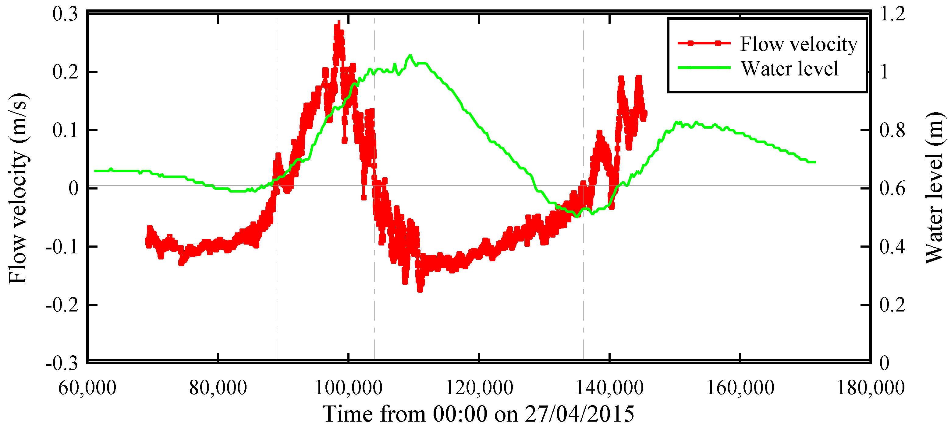
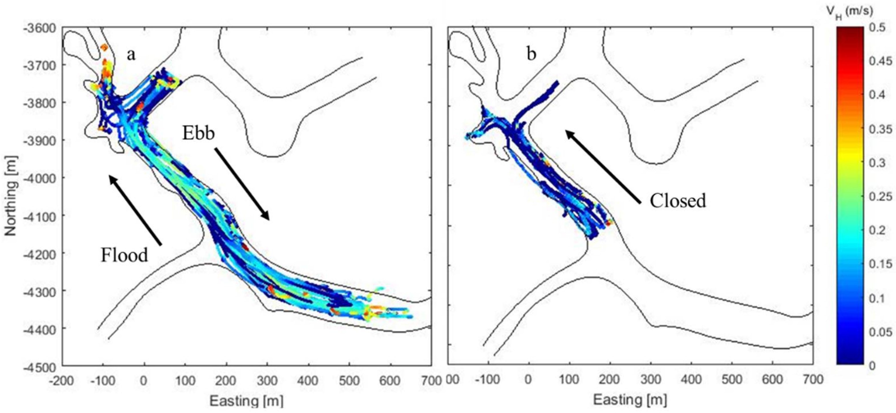
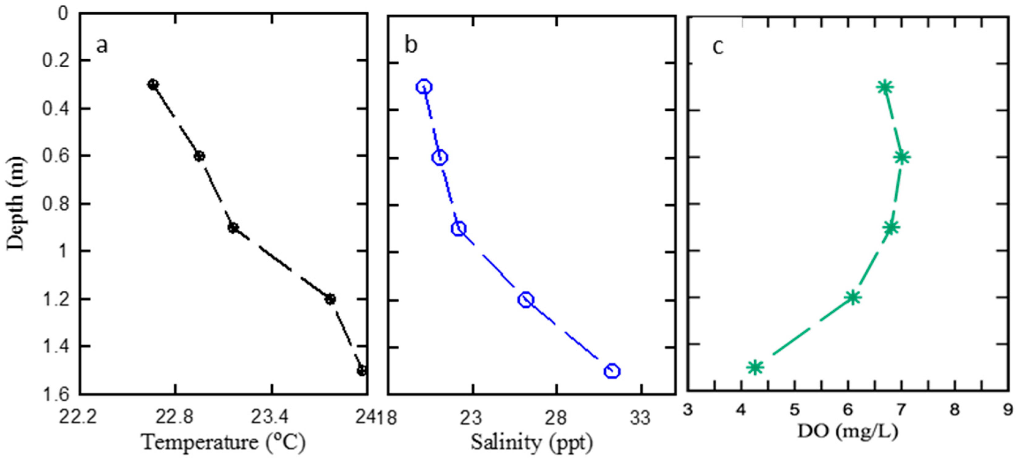
3.1. Basic Flow and Physiochemical Observations

During the open state experiment (E1) when the channel was connected to the ocean, measured salinity varied between 25 and 33 ppt. Horizontal transport was governed by river and tidal inflow. Comparison of water levels within the channel with tidal data from tidal gauge in the ocean indicated that the high and low waters in the channel lag the ocean by 2–3 h (not shown). The time series of mean flow velocity magnitude and the water level at Currimundi Lake is presented in Figure 4. Flow direction is indicated by the direction of the mean streamwise velocity component, which is positive in the upstream direction. The mean flow velocities were obtained using a moving average based on a 200 s average every 10 s along the entire dataset which is appropriate for estuaries of this type [37]. The channel exhibits a rapid and short flood tide compared to the ebb tide. The flood period occurred within 4-h with a peak velocity of 0.25 m s⁻¹, while ebb tide extended to a period up to 9-h with peak velocity limited to 0.18 m s⁻¹. The short-lived flood tide and the tidal asymmetry within the channel were likely influenced by the net outflow from Lake Kawana. The end (−3600–3700 m North; Figure 5) of the main channel exhibited secondary flows during the ebb, and higher flow velocity magnitudes >0.4 m s⁻¹ during the peak flood tide due to constriction of the channel. This accelerated flow in these narrow reaches, combined with the short-lived flood flow (Figure 5a), could accelerate streambank erosion in this portion of the channel, especially in areas not protected by woody riparian vegetation. As such, changes in channel morphology could occur in these upstream reaches.

Except for the locations in the constricted end of the main channel, variations in instantaneous velocity within the channel were limited to 0–0.3 m s⁻¹ and 0–0.15 m s⁻¹ during the open and closed states, respectively. The ebb and flood average flow velocity magnitude during the open state (E1) was approximately 0.1 m s⁻¹ and limited to 0.04 m s⁻¹ during the closed state (E2). These flow velocities are consistent with previous observations and hydrodynamic models of the channel [21].

Daytime vertical profiles of the physiochemical properties of the channel during the closed state (E2) indicated that the water column was strongly stratified in density from the salinity gradient (Figure 6b). With an insignificant vertical temperature gradient as observed during the closed state (E2), the source of stratification was likely connected with the freshwater inflow from stormwater run-off and from Lake Kawana, via the weir, after the inlet was closed (Figure 2c). The wind strength (speed < 5 m s⁻¹) observed near the surface was weak and unable to disrupt the stratified layer resulting in salinity gradient in the channel system. This inhibition of vertical mixing probably explains the depletion of oxygen near the channel bed through the consumption of oxygen by organisms in sediment-water layer (Figure 6).

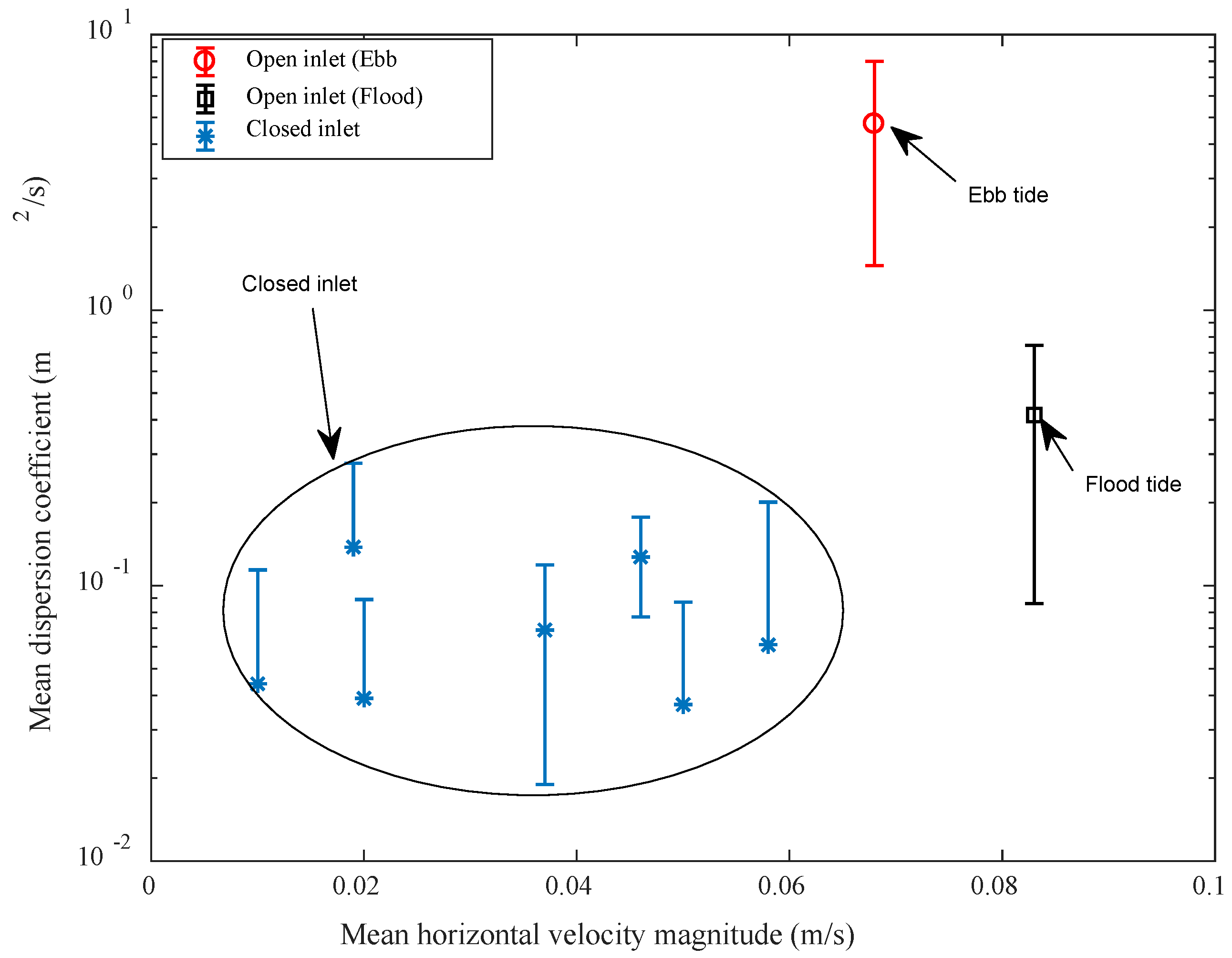
3.2. Horizontal Surface Dispersion Coefficient

In the open state (E1) during the flood time, the time variation of the cluster dispersion coefficient, K_c and centroid horizontal resultant velocity, V_H, varied throughout, which is a reflection of the tidal influence (Figure 7). However, temporal variation of K_c reflected different stages characterised by divergence (K_c > 0; Stages 1 and 2) and convergence (K_c < 0; Stages 3 and 4) of the cluster. Regions in the channel corresponding to these stages are identified in Figure 7b; drifter trajectories are colored by time. The magnitude of mean K_c for the stages was not significantly different from the overall mean. Of interest is the pronounced oscillation apparent in K_c, V_H, and cluster area manifested as two divergence/convergence events (Figure 8 and Figure 9a). This modulation of divergence and convergence has a period ~3000 s (e.g., Stage 2). Similar modulation of period ~3000 s can be observed in the time series of velocity of the cluster centroid and ADV (Figure 4). This corresponds to an internal resonance/wave of length 3.3 km in shallow water with an average depth, d ~ 0.5 m. This is probably due to resonance between the mouth and the fixed weir located 3.6 km from the channel inlet. The resonance effect is a reversible process manifested as cluster expansion/contraction [17,38]. However, this effect is expected to have some impact on the dynamics of the surface layer of the channel by destroying stratification and enhancing mixing.

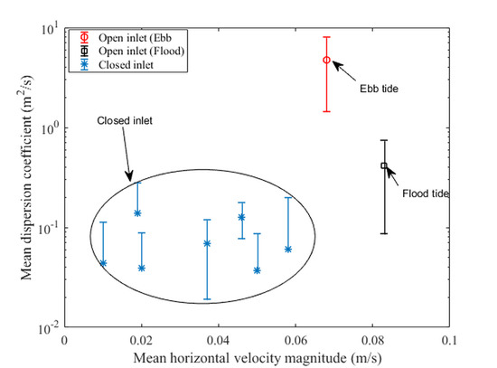
Effect of Inlet on the Dispersion Coefficient

A single deployment resulted in a range of cluster dispersion coefficients, K_c values and the data varied with the instantaneous effective length scale which is equivalent to the size of the patch. Due to the limited number of drifters in each individual cluster in some deployments, K_c values obtained from Equation (4) were noisy. Therefore, only the mean values over cluster deployments are reported in

Table 2. Cluster dispersion coefficient during the open state (E1) and closed state (E2).

Study	Experiment	Number of Drifters	Duration (s)	VH (m s−1)	Keff (m2 s−1)
E1 (tidal)					Contraction	Spreading	Effective
	Ebb	5–15	19,081	0.068	−1.440	5.070	4.700
	Flood	5–15	10,371	0.083	−0.410	0.430	0.420
E2 (Non-tidal)	C1	5	10,861	0.019	−0.140	0.140	0.140
	C2	3–5	11,461	0.010	−0.001	0.050	0.044
	C3	4	9781	0.050	−0.030	0.040	0.037
	C4	4	3721	0.020	−0.033	0.048	0.039
	C1	5	6721	0.058	−0.056	0.064	0.061
	C2	3–5	-	-	-	-	-
	C3	4	6241	0.037	−0.049	0.080	0.069
	C4	4	6181	0.046	−0.091	0.200	0.130

. The definition of a cluster allows for negative values of dispersion coefficient to be calculated, indicating cluster contraction, i.e., rather than spreading. Dispersion coefficients resulting from spreading and contraction are separately averaged for individual clusters and are determined by taking the mean over a deployment duration. Contraction of clusters of buoyant particles as opposed to spreading has been observed in environmental flows such as lakes, estuarine embayments and nearshores [35,38]. This phenomenon is usually related to a combination of physical processes—e.g., secondary flow, 3D contraction effect on quasi 2D flow, proximity to fronts and banks and internal waves (as discussed in Section 3.2), and dynamics of particles in a turbulent flow influenced by their inertia and drag [39].

The effective dispersion coefficients as a function of the mean cluster velocity are compared for the two inlet conditions (Figure 8). The results indicate that the ebb K_c = 4.73 ± 3.8 m² s⁻¹ is an order of magnitude greater than that of the flood tide and up to two orders of magnitude greater than values obtained when the inlet was closed. The ebb cluster diffusivities were similar to those (K = 6.5–9.9 m² s⁻¹) observed from dye tracer studies in natural rivers (depth = 0.58–1.56 m; width = 20–40 m) such as Green-Dumanish River and Powell River in the USA (Table 5.3; Fischer et al. [10]). A mean K_c value of 0.42 ± 0.34 m² s⁻¹ was obtained during the flood tide. This estimate is similar to K_c = 0.5 m² s⁻¹, obtained in a similar independent drifter experiment at a tidal inlet [40]. The estimate is also similar to the dispersion coefficient of 0.57 m² s⁻¹ obtained from absolute dispersion of high resolution drifters at Eprapah Creek, Australia, a smaller tidal channel [13].

The 1–2 orders of magnitude difference between the open and closed state dispersion coefficients highlight the role of tidal inflows in the horizontal transport and mixing within the channel. Mechanisms responsible for dispersion are those related to freshwater input and local wind effects. During the closed state (E2), wind intensity next to the channel surface was generally weak, less than 30% of the local wind velocity for the catchment (obtained at 4.5 m AHD). This is consistent with the boundary layer effect of mangroves and buildings [41] and explains the low dispersion coefficient.

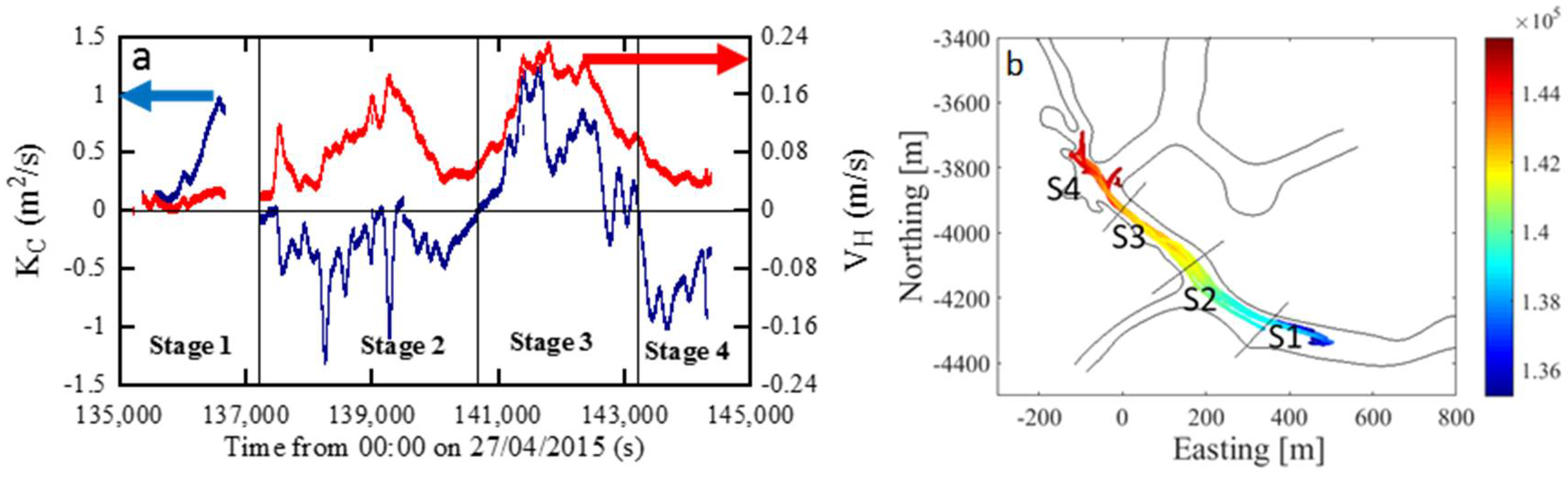
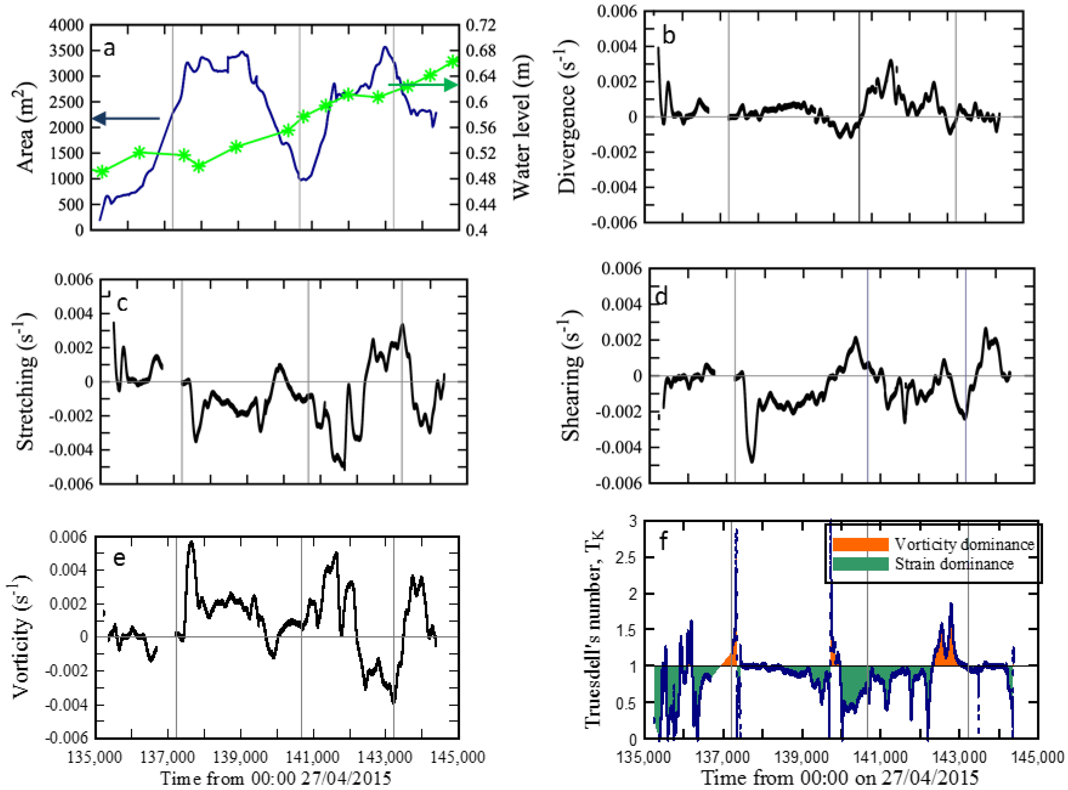
3.3. Differential Kinematic Properties

Differential kinematic properties (DKP) are particularly useful for describing the structure of relative motion of clustered particles and for relating the velocity field to dynamic processes. This is important for studying passive particle transport such as larvae, litter, and logs in response to the velocity gradient in an underlying flow field. Divergence provides an indication of vertical motion whilst vorticity is a diagnostic of external forcing such as interaction of tide with bottom topography or wind-induced forcing in the absence of tide [32]. Shearing and stretching deformation in the context of semi-enclosed waters are a function of horizontal boundary influences on cluster motion.

We first present the variation of DKPs observed during the flood tide for the open inlet condition. DKP varied temporally and spatially across the channel (Figure 9). Mean DKP values were in the order of 10⁻⁴ s⁻¹. Divergence and vorticity were predominantly positive, whilst shearing and stretching deformation were negative. Observed values were an order of magnitude larger than those observed in a non-tidal lake [17] and up to ten orders of magnitude lower than observed in the ocean [32]. The variation of T_K with time suggests that the channel was systematically dominated by strain fields for most of the flood tide during the baseline tidal condition (Figure 9f). Mixing during these periods was likely linked with interaction of the tide with irregular bathymetry, boundaries, and channel roughness elements such as riparian vegetation. However, some periods of vorticity dominance were observed. These periods corresponded to divergence-convergence interphase linked with internal resonance within the channel as identified from the cluster dispersion.

Mean DKP values were in the order of 10⁻⁴ s⁻¹ (

Table 3. Average kinematic differential properties of the Currimundi Lake during E1 and E2.

Study	Experiment	Duration	Differential Kinematic Properties				TK
E1 (tidal)		(s)	Vorticity × 10−4 s−1	Divergence × 10−4 s−1	Shearing × 10−4 s−1	Stretching × 10−4 s−1
	Ebb	19,081	**	8.91	**	**
	Flood	10,371	8.93	7.82	−2.35	−5.45	0.86
E2 (Non-tidal)	C1	10,861	−17.14	5.89	**	16.27
	C2	11,461	2.53	2.82	**	1.77
	C3	9781	16.04	4.71	−6.17	−18.96	0.64
	C4	3721	−10.88	−15.98	−28.53	−31.19	0.64
	C1	6721	9.83	17.04	−9.63	−5.19	0.70
	C2
	C3	6241	1.45	5.13	−4.44	−2.90	0.74
	C4	6181	61.03	11.24	5.04	−52.18	0.88

** indicates estimates which are not an order of magnitude higher than the uncertainty estimates from fixed observations.

). The standard deviation of DKP was, on average, an order of magnitude greater than the mean, indicating large variability and a limited number of particles in the clusters. This result indicates that on average the DKP of the channel was higher during the closed state (E2). Large values of DKP during the closed state (E2) are indicative of small spatial separation of the clusters. The drifter clusters tended not to separate great distances even 2 to 3-h after deployment, consistent with the observed lower dispersion coefficient. Consistent with wind driven transport, the vorticity and stretching effects were typically amplified during the closed state (E2) compared to the open state (E1). For all clusters and deployments, the time variation of T_K was predominantly less than 1, suggesting that dispersion of the clusters was dominated by strain fields rather than eddy-like structures. The dominance of the strain field within the channel implies that water parcels are stretched and sheared horizontally. This effect was probably associated with horizontal velocity shearing resulting from the interactions of the tide with topographic structures within the channel (e.g., bars, banks, and vegetation) during the open state and wind-driven flow forced against the banks during the closed state.

3.4. Horizontal Dispersion Mechanisms within the Channel

3.4.1. Open State (E1)

During the open state (E1), horizontal dispersion in the natural channel is influenced by the combination of the dispersive effect of wind, tide, and river currents. In a long, narrow channel such as Currimundi Lake, dispersion resulting from wind-driven currents at moderate wind speeds (e.g., 0–5 m s⁻¹) observed during the field study, is probably insignificant compared with the influences of the tide and river. The physical mechanisms for horizontal dispersion based on the competition between the tide and freshwater inflow are related to the additive effects of turbulence, shear dispersion, tidal trapping, and pumping.

Turbulent mixing resulting from the flow boundaries such as beds and banks is parameterised as eddy diffusivity, K_turb. Assuming well-mixed conditions, K_turb could be expressed as [8]:

$$K_{turb}\approx C_D{U}_{t}h$$

(8)

where C_D is the drag coefficient relating the square of depth-averaged velocity to the bottom stress, U_t is the amplitude of the tidal velocity, and h is the averaged water depth. Using a typical range of U_t = 0.05–0.3 m s⁻¹ and h = 1–2 m observed during the open state (E1) and assuming C_D = 0.003 after [42], the vertical mixing within Currimundi Lake can be estimated as K_turb = 1.5–18 × 10⁻⁴ m² s⁻¹.

Horizontal shear dispersion results from the dispersive effects of transverse velocity gradients in open channel flow. For a symmetrical open channel, the flow at the middle of the channel is faster relative to the sides because of friction loss along streambanks. The concept of shear dispersion in open channel turbulent flow is analysed by [27], who assumed a logarithmic turbulent velocity. The concept has been extended to oscillatory tidal flows [10]. The resulting horizontal dispersion, K_shear, can be approximated by the tidal velocity and width, W as:

$$K_{shear}\approx (0.1-0.2)U_{t}W$$

(9)

Using the observed field tidal velocity and an average channel width, W ~ 50 m, K_shear is estimated between 0.25–3 m² s⁻¹ during the open state (E1).

Tidal trapping occurs as a result of geometrical variation that leads to a difference in the phase of tidal flow between the main channel and branching channels [8]. Okubo [43] used an analytical approach to estimate the dispersion coefficient associated with this phenomenon based on the trapped volume in the branching channels, the tidal excursion length, L, and the tidal velocity amplitude:

$$K_{trap}\approx 0.25r{U}_t{L}_t$$

(10)

Assuming a trapped volume r ~ 0.2 based on the ratio of the volume of the branching and main channels in Currimundi Lake, a tidal excursion length L_t ~ 2000 m based on the tidal range, and depth and length of the main channel, K_trap is estimated to vary between 5–30 m² s⁻¹. The tidal pumping effect, on the other hand, describes the net transport that is caused by the difference between the ebb and flood tidal currents [8]. This effect may significantly influence the horizontal dispersion in Currimundi Lake considering the difference in the flow behaviour between the flood and ebb tides observed with the ADV and drifters. However, a resulting dispersion coefficient from tidal pumping was not estimated due to difficulty in estimating the residual recirculation owing to the complexity of the channel network and dead ends.

By comparing the observed K_c values for different experiments with those predicted using approximate solutions for individual mechanisms, the dominant underlying mechanisms can be explained. The K values observed during the open state (E1) were larger than the inherent eddy diffusivity within the channel, indicating dominance of larger scale processes. The flood tide mean K = 0.42 m² s⁻¹ was similar in magnitude with that predicted by the shear dispersion mechanism. The ebb tide mean K = 4.73 m² s⁻¹, on the other hand, was similar in magnitude to that predicted by a trapping mechanism. This suggests that the horizontal dispersion within the channel during an open state is dominated by large-scale mechanisms such as horizontal shear dispersion and tidal trapping. Trapping within the channel could be linked to the influence of the narrow and shallow channel branches compared with the main channel. This geometrical effect reduces the resistance of the channel branches to inertia forces leading to quicker ebbing in the channel branches and potentially increases in erosive forces along banks. In addition, Currimundi Lake is connected to Lake Kawana via a weir head located at 0.65 m AHD. This structure restricts the over-passage of flow at tidal elevations less than 0.65 m AHD while freshwater is supplied into the system creating an induced trapping and tidal asymmetry.

3.4.2. Closed State (E2)

During the closed state (E2), the tidal effect was absent. Therefore, the driving forces for horizontal transport were expected to be from horizontal density gradients and wind forcing. The water level was fairly constant and there was no significant stormwater runoff into the channel during the study period. There was no significant difference between the density between the pontoon and the bridge. Therefore, the influence of horizontal density gradient currents within the channel was negligible. To examine the influence of wind on horizontal transport, drifter motion and wind velocity measured 0.5 m above the water surface during the closed state (E2) are presented using a rose diagram (Figure 10). To obtain a better visual match with the drifter motion, the wind rose is presented in terms of the direction to where the wind was blowing (Figure 10), i.e., rotated by 180^o compared to conventional wind rose diagrams, and transformed to a local coordinate system. The directions illustrated in the wind rose approximately represent the ensemble average drifter direction and speed in a Eulerian perspective at a particular interval and do not necessarily represent the Lagrangian trajectory [44]. A comparison of the drifter rose with the wind rose should therefore be interpreted cautiously. The near surface wind speed was predominantly between 1–5 m s⁻¹ blowing in a N-NW direction. The drifter speeds were mainly between 0–0.15 m s⁻¹ and drifted towards N-NW. The result showed that the drifter speeds were between 0–5% of the wind speed and within 20° of the wind direction. This suggests a significant contribution of wind to the dynamics of the surface flow during the closed state (E2) at low to moderate wind speeds observed within the channel. The drifter motion did display wind driven transport, such as net deflection to the left of the wind direction as expected in the southern hemisphere. However, the net angle of deflection over ~0.5 m of the channel was limited to 20° compared to the expected 45° Ekman deflection at the surface. This was largely due to the small size and elongation of the main channel that substantially modified the Ekman influence.

3.5. Implications for Current Lake Management Strategies

Several lake management issues can be informed by these results: the horizontal dynamics of particles in the channel litter accumulation, and water quality in the upstream reaches, whilst pest control remains of concern throughout the ICOLL.

Biting midge management is a major concern in Australian coastal areas and across many other tropical and sub-tropical areas. Midge larvae are difficult to control by direct application of larvicides in their breeding sites because they are deposited in mud and wet soils high in organic matter [45]. While tidal cycles have been observed to aid breeding of intertidal biting midge species [19], recent research has shown that the larvae of many species are not able to survive inundation for a long period [20], thus creating an opportunity for larvae control at sites next to channel banks. Midge larvae management conducted by the local government in Currimundi Lake entails the annual drowning of the larvae laid in sandy banks by blocking Currimundi Lake inlet for a period of approximately 14 days; this is the typical lifespan of biting midge in mid-summer [19]. The results presented herein support the practice of closing the channel inlet at a period coinciding with the peak midge breeding period as an effective control strategy. This is because dispersion was lower and significant flow fluctuations were absent during the closed inlet experiment; therefore, larvae in the banks of the channel likely remain inundated as the water level rises. In addition, the vertical profile water quality parameters showed a depletion of oxygen closer to the bed, thus reducing larval access to oxygen.

Litter in southeast Queensland is dominated by cigarette butts [28,46]. Currimundi Lake area attracts a large number of tourists because of the combination of a sheltered inlet in close proximity to a surfing beach. To reduce the impact of litter on the water quality, catchment community groups actively pursue litter clean ups. The strong direction coherence of the motion of drifters with wind during the closed state (E2) indicates that wind information can provide some guidance for litter management. During the closed condition, the flow is dominated by the wind and dispersion coefficients are an order of magnitude lower, resulting in less spreading of litter (see Figure 5, Figure 8 and Figure 10) during the closed state (E2). The dominant wind direction for Lake Currimundi is SE-S and litter will therefore accumulate along the NW-N banks of the lake.

4. Summary and Conclusions

The dynamics and horizontal dispersion of Currimundi Lake, a shallow intermittently closed and open lake and lagoon, were studied to examine the dispersion coefficients and dispersion mechanisms for different inlet conditions and their implications on some key management issues. The analysis of drifter deployments, ADV observation, and physiochemical properties highlight a significant contribution of tide in the flow dynamics of the channel. A fixed ADV mounted near the surface and a GPS-tracked drifter during the open and closed states were used to observe the flow dynamics of the channel. The analysis of the water levels within the channel and on the ocean side indicated that the channel exhibited high and low tides that lagged the ocean within 2–3 h. Generally, the inflow and outflow velocities were weak with speeds <0.25 m s⁻¹. The channel exhibited a rapid flood tide flow compared to the ebb tide. This accelerated flow, combined with short-lived flood flow, may modify the upstream channel morphology. The channel was stratified during the closed system, likely linked with freshwater inflow, low wind forcing, and low solar insolation [6]. The freshwater pumped into the lake likely keeps the channel connected to the ocean [21] and also induced salinity gradient during the closed system. The results here further suggest that the freshwater input induced tidal asymmetry and enhanced horizontal dispersion within the channel.

Importantly, the closed state exhibited a dispersion coefficient up to two orders of magnitude less than those observed during the open state (E1), indicating that the absence of tide due to the blocked inlet reduced transport and horizontal mixing processes within the channel. During the open state (E1), it was found that the dispersion coefficient varied drastically for different tidal phases with the ebb tide average dispersion coefficient K ~ 4.7 m² s⁻¹ an order of magnitude greater than flood estimates.

The comparison of the observed dispersion coefficients with theoretical estimates showed that the tidal trapping effect and the tidal-induced horizontal velocity gradient likely explained the horizontal transport and dispersion during the open inlet state. During the closed state (E2), the drifters followed the wind driven surface flow with drifter speeds between 0–5% of the near water surface wind speed and aligned to the wind direction within 20°. This indicated a modified Ekman surface transport during the closed inlet. This highlights that accurate wind information is required for modelling the transport of particles and the physiochemical properties of the channel during the closed inlet condition. An ongoing analysis examines the response of channel flow dynamics and the processes involved in restoration of water in the channel immediately after a mechanical opening operation.

References

1. Gale, E.; Pattiaratchi, C.; Ranasinghe, R. Processes driving circulation, exchange and flushing within intermittently closing and opening lakes and lagoons. Mar. Freshw. Res. 2007, 58, 709–719. [Google Scholar] [CrossRef]
2. Pollard, D. Opening regimes and salinity characteristics of intermittently opening and permanently open coastal lagoons on the south coast of New South Wales. Wetl. Aust. J. 1994, 13, 16–35. [Google Scholar]
3. Roy, P.; Williams, R.; Jones, A.; Yassini, I.; Gibbs, P.; Coates, B.; West, R.; Scanes, P.; Hudson, J.; Nichol, S. Structure and function of south-east Australian estuaries. Estuar. Coast. Shelf Sci. 2001, 53, 351–384. [Google Scholar] [CrossRef]
4. Milbrandt, E.C.; Bartleson, R.D.; Coen, L.D.; Rybak, O.; Thompson, M.A.; DeAngelo, J.A.; Stevens, P.W. Local and regional effects of reopening a tidal inlet on estuarine water quality, seagrass habitat, and fish assemblages. Cont. Shelf Res. 2012, 41, 1–16. [Google Scholar] [CrossRef]
5. Schallenberg, M.; Larned, S.T.; Hayward, S.; Arbuckle, C. Contrasting effects of managed opening regimes on water quality in two intermittently closed and open coastal lakes. Estuar. Coast. Shelf Sci. 2010, 86, 587–597. [Google Scholar] [CrossRef]
6. Gale, E.; Pattiaratchi, C.; Ranasinghe, R. Vertical mixing processes in intermittently closed and open lakes and lagoons, and the dissolved oxygen response. Estuar. Coast. Shelf Sci. 2006, 69, 205–216. [Google Scholar] [CrossRef]
7. Wiles, P.J.; van Duren, L.A.; Häse, C.; Larsen, J.; Simpson, J.H. Stratification and mixing in the Limfjorden in relation to mussel culture. J. Mar. Syst. 2006, 60, 129–143. [Google Scholar] [CrossRef]
8. Geyer, W.R.; Signell, R.P. A reassessment of the role of tidal dispersion in estuaries and bays. Estuaries 1992, 15, 97–108. [Google Scholar] [CrossRef]
9. Uncles, R.J.; Torres, R. Estimating dispersion and flushing time-scales in a coastal zone: Application to the Plymouth area. Ocean Coast. Manag. 2013, 72, 3–12. [Google Scholar] [CrossRef]
10. Fischer, H.B.; List, E.J.; Koh, R.C.; Imberger, J.; Brooks, N.H. Mixing in Inland and Coastal Waters; Academic Press: New York, NY, USA, 1979; ISBN 0122581504. [Google Scholar]
11. Riddle, A.; Lewis, R. Dispersion experiments in UK coastal waters. Estuar. Coast. Shelf Sci. 2000, 51, 243–254. [Google Scholar] [CrossRef]
12. Shaha, D.; Cho, Y.-K.; Kwak, M.-T.; Kundu, S.; Jung, K. Spatial variation of the longitudinal dispersion coefficient in an estuary. Hydrol. Earth Syst. Sci. 2011, 15, 3679–3688. [Google Scholar] [CrossRef] [Green Version]
13. Suara, K.A.; Wang, C.; Feng, Y.; Brown, R.J.; Chanson, H.; Borgas, M. High resolution GNSS-tracked drifter for studying surface dispersion in shallow water. J. Atmos. Ocean. Technol. 2015, 32, 579–590. [Google Scholar] [CrossRef]
14. George, R.; Largier, J.L. Description and performance of finescale drifters for coastal and estuarine studies. J. Atmos. Ocean. Technol. 1996, 13, 1322–1326. [Google Scholar] [CrossRef]
15. Tseng, R.S. On the dispersion and diffusion near estuaries and around islands. Estuar. Coast. Shelf Sci. 2002, 54, 89–100. [Google Scholar] [CrossRef]
16. Suara, K.A.; Brown, R.J.; Borgas, M. Eddy diffusivity: A single dispersion analysis of high resolution drifters in a tidal shallow estuary. Environ. Fluid Mech. 2016, 16, 923–943. [Google Scholar] [CrossRef]
17. Stocker, R.; Imberger, J. Horizontal transport and dispersion in the surface layer of a medium-sized lake. Limnol. Oceanogr. 2003, 48, 971–982. [Google Scholar] [CrossRef] [Green Version]
18. Bowden, K.F. Horizontal mixing in the sea due to a shearing current. J. Fluid Mech. 1965, 21, 83–95. [Google Scholar] [CrossRef]
19. Kettle, D.S.; Edwards, P.B.; Barnes, A. Factors affecting numbers of Culicoides in truck traps in coastal Queensland. Med. Vet. Entomol. 1998, 12, 367–377. [Google Scholar] [CrossRef] [PubMed]
20. Lühken, R.; Steinke, S.; Wittmann, A.; Kiel, E. Impact of flooding on the immature stages of dung-breeding culicoides in northern europe. Vet. Parasitol. 2014, 205, 289–294. [Google Scholar] [CrossRef] [PubMed]
21. Tomlinson, R.; Williams, P.; Richards, R.; Weigand, A.; Schlacher, T.; Butterworth, V.; Gaffet, N. Lake Currimundi Dynamics Study Final Report Volume 1 and 2; Griffith Centre for Coastal Management, Griffith University: Southport, Australia, 2010. Available online: https://www.sunshinecoast.qld.gov.au/Environment/Rivers-and-Coast/Lake-Currimundi-Dynamics-Study (accessed on 1 May 2017).
22. Okubo, A. Oceanic diffusion diagrams. Deep Sea Res. Oceanogr. Abstr. 1971, 18, 789–802. [Google Scholar] [CrossRef]
23. Suara, K.; Ketterer, T.; Fairweather, H.; McCallum, A.; Vanaki, S.M.; Allan, C.; Brown, R. Cluster Dispersion of Low-Cost GPS-Tracked Drifters in a Shallow Water. Proceedings of 10th Australasian Heat and Mass Transfer Conference, Brisbane, Australia, 14–15 July 2016; Australasian Fluid and Thermal Engineering Society: Brisbane, Australia, 2016. [Google Scholar]
24. ABM. Australian Government Bureau of Meteorology. Daily Global Solar Exposure. 2015. Available online: http://www.bom.gov.au/jsp/ncc/cdio/weatherData/av?p_nccObsCode=193&p_display_type=dailyDataFile&p_startYear=2015&p_c=-336226903&p_stn_num=040998 (accessed on 11 April 2018).
25. SCC. More Than 90% Pesky Midges Wiped Out. Available online: https://www.sunshinecoast.qld.gov.au/Council/News-Centre/Currimundi-Lake-reopening-18-October-2016 (accessed on 12 May 2017).
26. Suara, K.A. Development and Use of GPS-Based Technology to Study Dispersion in Shallow Water. Ph.D. Thesis, Science and Engineering Faculty, Queensland University of Technology, Brisbane, Australia, 2017. [Google Scholar]
27. Elder, J.W. The dispersion of marked fluid in turbulent shear flow. J. Fluid Mech. 1959, 5, 544–560. [Google Scholar] [CrossRef]
28. Madhani, J.T.; Dawes, L.A.; Brown, R.J. A perspective on littering attitudes in Australia. Environ. Eng. J. Soc. Sustain. Environ. Eng. 2009, 9, 13–20. [Google Scholar]
29. Suara, K.; Wang, H.; Chanson, H.; Gibbes, B.; Brown, R. Response of GPS-tracked drifters to wind and water currents in a tidal estuary. IEEE J. Ocean. Eng. 2018, in press. [Google Scholar]
30. List, E.J.; Gartrel, G.; Winant, C.D. Diffusion and dispersion in coastal waters. J. Hydraul. Eng. 1990, 116, 1158–1179. [Google Scholar] [CrossRef]
31. Okubo, A.; Ebbesmeyer, C.C. Determination of vorticity, divergence, and deformation rates from analysis of drogue observations. Deep Sea Res. Oceanogr. Abstr. 1976, 23, 349–352. [Google Scholar] [CrossRef]
32. Molinari, R.; Kirwan, A.D., Jr. Calculations of differential kinematic properties from Lagrangian observations in the western Caribbean sea. J. Phys. Oceanogr. 1975, 5, 483–491. [Google Scholar] [CrossRef]
33. Truesdell, C. The Kinematics of Vorticity; Indiana University Press: Bloomington, IN, USA, 1954. [Google Scholar]
34. Okubo, A. Some speculation on oceanic diffusion diagrams. Rapp. P.-V. Reun. Cons. Int. Explor. Mer. 1974, 167, 77–85. [Google Scholar]
35. Suara, K.; Chanson, H.; Borgas, M.; Brown, R.J. Relative dispersion of clustered drifters in a small micro-tidal estuary. Estuar. Coast. Shelf Sci. 2017, 194, 1–15. [Google Scholar] [CrossRef] [Green Version]
36. Johnson, D.; Stocker, R.; Head, R.; Imberger, J.; Pattiaratchi, C. A compact, low-cost GPS drifter for use in the oceanic nearshore zone, lakes, and estuaries. J. Atmos. Ocean. Technol. 2003, 20, 1880–1884. [Google Scholar] [CrossRef]
37. Chanson, H.; Brown, R.J.; Trevethan, M. Turbulence measurements in a small subtropical estuary under king tide conditions. Environ. Fluid Mech. 2012, 12, 265–289. [Google Scholar] [CrossRef] [Green Version]
38. Manning, J.P.; Churchill, J.H. Estimates of dispersion from clustered-drifter deployments on the southern flank of Georges Bank. Deep Sea Res. Part II 2006, 53, 2501–2519. [Google Scholar] [CrossRef] [Green Version]
39. Pinton, J.-F.; Sawford, B.L. A Lagrangian view of turbulent dispersion and mixing. In Ten Chapters in Turbulence; Davidson, P.A., Kaneda, Y., Sreenivasan, K.R., Eds.; Cambridge University Press: New York, NY, USA, 2012. [Google Scholar]
40. Spydell, M.S.; Feddersen, F.; Olabarrieta, M.; Chen, J.; Guza, R.T.; Raubenheimer, B.; Elgar, S. Observed and modeled drifters at a tidal inlet. J. Geophys. Res. Oceans 2015, 120, 4825–4844. [Google Scholar] [CrossRef] [Green Version]
41. Manwell, J.F.; McGowan, J.G.; Rogers, A.L. Wind characteristics and resources. In Wind Energy Explained; John Wiley & Sons, Ltd.: West Sussex, UK, 2009; pp. 23–89. [Google Scholar]
42. Geyer, W.R.; Trowbridge, J.H.; Bowen, M.M. The dynamics of a partially mixed estuary. J. Phys. Oceanogr. 2000, 30, 2035–2048. [Google Scholar] [CrossRef]
43. Okubo, A. Effect of shoreline irregularities on streamwise dispersion in estuaries and other embayments. Neth. J. Sea Res. 1973, 6, 213–224. [Google Scholar] [CrossRef]
44. Delpeche-Ellmann, N.; Torsvik, T.; Soomere, T. A comparison of the motions of surface drifters with offshore wind properties in the Gulf of Finland, the Baltic sea. Estuar. Coast. Shelf Sci. 2016, 172, 154–164. [Google Scholar] [CrossRef]
45. Carpenter, S.; Mellor, P.S.; Torr, S.J. Control techniques for Culicoides biting midges and their application in the UK and northwestern Palaearctic. Med. Vet. Entomol. 2008, 22, 175–187. [Google Scholar] [CrossRef] [PubMed]
46. Madhani, J.T. The Hydrodynamic and Capture/Retention Performance of a Gross Pollutant Trap. Ph.D. Thesis, Faculty of Built Environment and Engineering, Queensland University of Technology, Brisbane, Australia, 2010. [Google Scholar]
Figure 1. (a) Aerial view of Currimundi Lake catchment (Longitude 153.13° E, Latitude 26.763° S Nearmap, 2015); (b) Expanded view of the Currimundi Lake main channel; X—water quality monitoring station. (c) A cluster of four GPS-tracked drifters ~5 min after deployment. (d) Rendered drawing of the High (HR) & Low (LR) resolution drifters hulls.
Water 10 00776 g001
Figure 2. Time series of: (a) Water level around E1, (b) Salinity around E1, (c) Water level around E2 (d) Salinity around E2; Measured at the bridge location marked X (Figure 1).
Water 10 00776 g002
Figure 3. Surveyed cross-section, next to the pontoon (Figure 1b), conducted during the closed state (E2) (9 September 2015) facing downstream; location of ADV during the open state (E1) relative to the free surface is shown.
Water 10 00776 g003
Figure 4. Time series of mean flow velocity magnitude and water level at Currimundi Lake.
Water 10 00776 g004
Figure 5. “Spaghetti” plot showing the drifter trajectory coloured by the horizontal velocity magnitude for drifter deployments during study: arrow indicate the main flow direction. (a) E1 under open inlet condition, (b) E2 under closed inlet condition.
Water 10 00776 g005
Figure 6. Vertical profile of the physiochemical properties of Currimundi Lake during the closed state E2, 9 September 2015 at the Pontoon (Figure 1). (a) Temperature, (b) Salinity, (c) Dissolved oxygen.
Water 10 00776 g006
Figure 7. (a) Time variation of dispersion coefficient (blue) and centroid velocity magnitude (red) of drifter cluster during open state (E1) during the flood experiment, (b) Drifter trajectory coloured by time (s), with vertical lines separating Stages S1–S4 in (a) corresponding to cross lines separating S1–S4 in (b). Note: the number of active drifter for the calculation was 5–15; periods with drifter numbers, n < 5 are not included.
Water 10 00776 g007
Figure 8. Comparison of effective cluster dispersion coefficient in the open (E1) and closed (E2) states; the error-bars represents the 1 standard deviation length around the mean value.
Water 10 00776 g008
Figure 9. Time variations of cluster properties during open state (E1) Flood experiment: (a) Area and water level (m) in channel (* green line), (be) differential kinematic properties (Equation (6)), (b) Divergence, (c) Stretching, (d) Shearing, (e) Vorticity, (f) Time variation of Truesdell’s kinematic (blue line) vorticity number (Equation (7)). Note: the number of active drifters 5–15; periods with drifter numbers, n < 5 are not included.
Water 10 00776 g009
Figure 10. Wind (a) and drifter (b) “roses” for the period of drifter deployment during the closed state (E2) on 9 September 2015. To more easily match the drift directions, the wind roses are shown with the directions that the winds were blowing. Both wind and drifter speeds are given in m s−1.
Water 10 00776 g010