Assessing Environmental Flow Targets Using Pre-Settlement Land Cover: A SWAT Modeling Application


1
School of Natural Resources, University of Missouri, 203-T ABNR Building, Columbia, MO 65211, USA
2
Institute of Water Security and Science, West Virginia University, 4121 Agricultural Sciences Building, Morgantown, WV 26506, USA
3
Davis College, Schools of Agriculture and Food, and Natural Resources, West Virginia University, 4121 Agricultural Sciences Building, Morgantown, WV 26506, USA
*
Author to whom correspondence should be addressed.
Water 2018, 10(6), 791; https://doi.org/10.3390/w10060791
Submission received: 3 May 2018
/
Revised: 10 June 2018
/
Accepted: 13 June 2018
/
Published: 15 June 2018
(This article belongs to the Section Water Resources Management, Policy and Governance)
Abstract
:Determining environmental flow requirements to sustain aquatic ecosystem health remains a challenge. The purpose of this research was to quantify the extent of current flow alterations relative to baseline hydrologic conditions of a simulated historic flow regime prior to anthropogenic flow disturbance (i.e., pre-settlement flows). Results allowed assessment of the efficacy of environmental flow targets based on pre-settlement land cover in a contemporary mixed-land-use catchment (i.e., urban, agricultural, and forested). Pre-settlement flows were simulated using the Soil and Water Assessment Tool (SWAT). Pre-settlement land cover, based on soil physical characteristics, was used to simulate pre-settlement flows with the SWAT model. Environmental flow targets were calculated for each flow element of a historic flow regime (magnitude, frequency, duration, timing, and rate of change). Urban (20% of watershed area) and agricultural development (42% of watershed area) were correlated to decreased median daily stream flow by 0.8 m3 s−1 (percent difference = −115%), increased maximum daily flow by 22 m3 s−1 (percent difference = 13%), and a 34% increase in daily flow variability. High flow frequency increased by 45–76% following development. Results highlight a need for consideration of environmental flow targets appropriate for watersheds already modified by existing land use, and point to a need for long-term, broad-scale, and persistent efforts to develop achievable environmental flow recommendations, particularly in rapidly urbanizing mixed-land-use watersheds.
1. Introduction
Environmental flows define the flow regime important to sustain the ecological health of receiving waters [1,2]. A review of the literature by Poff et al. [2] indicated that most environmental flow studies have included investigations of flow regimes altered by hydrologic infrastructure (e.g., hydropower dams, levees, and impoundments) or excessive surface water extractions that can substantially modify flow regimes. Historically, the management focus was on sustaining a minimum flow level (i.e., low flows) in streams and rivers impacted by hydrologic infrastructure and surface water extraction, assuming that adequate low flows would secure ecological integrity [3,4]. While low flow requirements have helped to mitigate aquatic habitat loss in streams and rivers, it is now recognized that regulating minimum flows alone will not sustain aquatic ecosystem health [4]. All elements across the continuum of a flow regime are important for ecosystem function [3,4,5,6]. Thus, environmental flow recommendations now include flow magnitude, frequency, timing, duration, and rate of change targets to restore historic flow regimes prior to anthropogenic flow disturbance, and thereby promote aquatic ecosystem health, protect ecosystem services, and secure water resources for use [2,4].
There are an increasing number of studies being undertaken to quantitatively assess the environmental flow targets necessary to mitigate ecological degradation due to rapid human development (particularly urbanization) [7,8]. However, the current pace of impairment due to rapid development continues to exceed management efforts globally [9,10,11]. To meet the pace of impairment, there has been a call from the literature for regional environmental flow assessments necessary to restore flow regimes [2,12]. Frameworks that outline analytical and modeling approaches, like the Hydroecological Integrity Assessment Process (HIP) [5] and Ecological Limits of Hydrologic Alteration (ELOHA) [2], have been provided to aid development of environmental flow standards appropriate for regional comprehensive flow management. Additional information regarding environmental flow methods have been reviewed by Pastor et al. [11].
Regional environmental flow assessments using the HIP and ELOHA frameworks involve building a hydrologic foundation of baseline and current flow regimes. However, baseline conditions of historic flow regimes are often not available for an area of interest. In such a case, end users can simulate baseline hydrologic conditions using watershed-scale hydrologic models [5,6]. Such information can be used to develop a priori environmental flow recommendations (i.e., flow targets) necessary to protect ecological health and public interests of water resources.
The Soil and Water Assessment Tool (SWAT) is an example of an internationally accepted, physically based, semi-distributed watershed-scale continuous time hydrologic model [13]. The SWAT model was designed to simulate long-term influences of climate, topography, soils, land use, and management operations on water, sediment, and chemical yields without large investments of resources (e.g., time, money, and labor). The SWAT model is an appropriate choice for simulating historic environmental flow regimes [5]. Inputs of pre-development land cover with native vegetation can be estimated using important soil series information. For example, native vegetation dependent on climate and soils properties can be found in Ecological Site Descriptions (ESD) and Official Soils Series Descriptions (OSD) developed by United States Department of Agriculture National Resource Conservation Service (USDA-NRCS) [14,15]. The SWAT model could be used as a standard for the development of baseline hydrology in regions where flow is impaired and observed baseline conditions are not available. However, there is a need to test the efficacy of using SWAT to simulate pre-settlement baseline hydrologic conditions important for regional environmental flow assessment.
When performing regional environmental flow assessments, it is important to consider a suite of different hydrologic indices to represent all key components of the flow regime [2,5]. U.S. Geological Survey (USGS) employees have developed and provided a statistical package named EflowStats in R computer language that can be used to calculate 171 “ecologically relevant” hydrologic indices for environmental flow analysis [6]. The hydrologic indices include in EflowStats that were determined to be ecologically relevant and were derived from multiple hydroecological peer-reviewed articles [16,17,18,19,20,21,22,23,24,25,26,27,28,29], as noted by Olden and Poff [6]. EflowStats is a reimplementation of the Hydrologic Index Tool (HIT) [30]. Unlike the original HIT, EflowStats has been redesigned to use hydrologic time series data and is not restricted to data formats used by the USGS National Water Information System.
EflowStats is a robust tool capable of calculating multiple complex time series calculations in a matter of seconds. However, many of the resulting values of those hydrologic indices are commonly correlated. For example, many high flow magnitude variables have been found to be correlated [23]. Such problems with multicollinearity can invalidate statistical assumptions, resulting in redundancy of the statistical significance of a particular flow element and/or group of hydrologic indices, in which case, it is recommended to reduce redundancy of hydrologic indices using a multivariate statistical approach, for example, principal component analysis (PCA) [5,6,26]. Results from EflowStats and PCA can be used to succinctly define key elements of an environmental flow regime.
Kennen et al. [5] completed a regional HIP analysis in Missouri streams. The HIP methods can be used to meet the call from the literature for broad-scale regional methodologies needed to promote aquatic ecosystem health, protect ecosystem services, and secure water resources for use in the USA [2]. While it is clear that HIP can be applied at statewide scales to generate ecologically relevant hydrologic indices for each stream type, there is a need to validate those results at scales appropriate for management (i.e., the watershed scale) in reference to mixed-land-use watersheds, where land use has been shown to alter stream flow.
The purpose of this research is to quantify the extent of current flow alterations, relative to baseline hydrologic conditions of a historic flow regime (i.e., simulated pre-settlement flows) to assess the efficacy of environmental flow targets based on pre-settlement land cover in a contemporary mixed-land-use catchment (i.e., urban, agricultural, and forested). Sub-objectives were to: (i) quantify baseline (i.e., SWAT simulated pre-settlement flows) and observed current flows, (ii) select, from the 171 ecologically relevant hydrologic indices provided in EflowStats, a subset of statistically significant hydrologic indices to represent each key element of the flow regime, and (iii) generate environmental flow targets using 7 years of stream flow data collected from five nested gauging sites in a mixed-land-use watershed that is representative of the central USA. Additionally, results from this exemplar environmental flow SWAT modeling application will be discussed in general terms to highlight key findings from the current work, with implications to other mixed-land-use watersheds globally.
2. Materials and Methods
2.1. Study Site
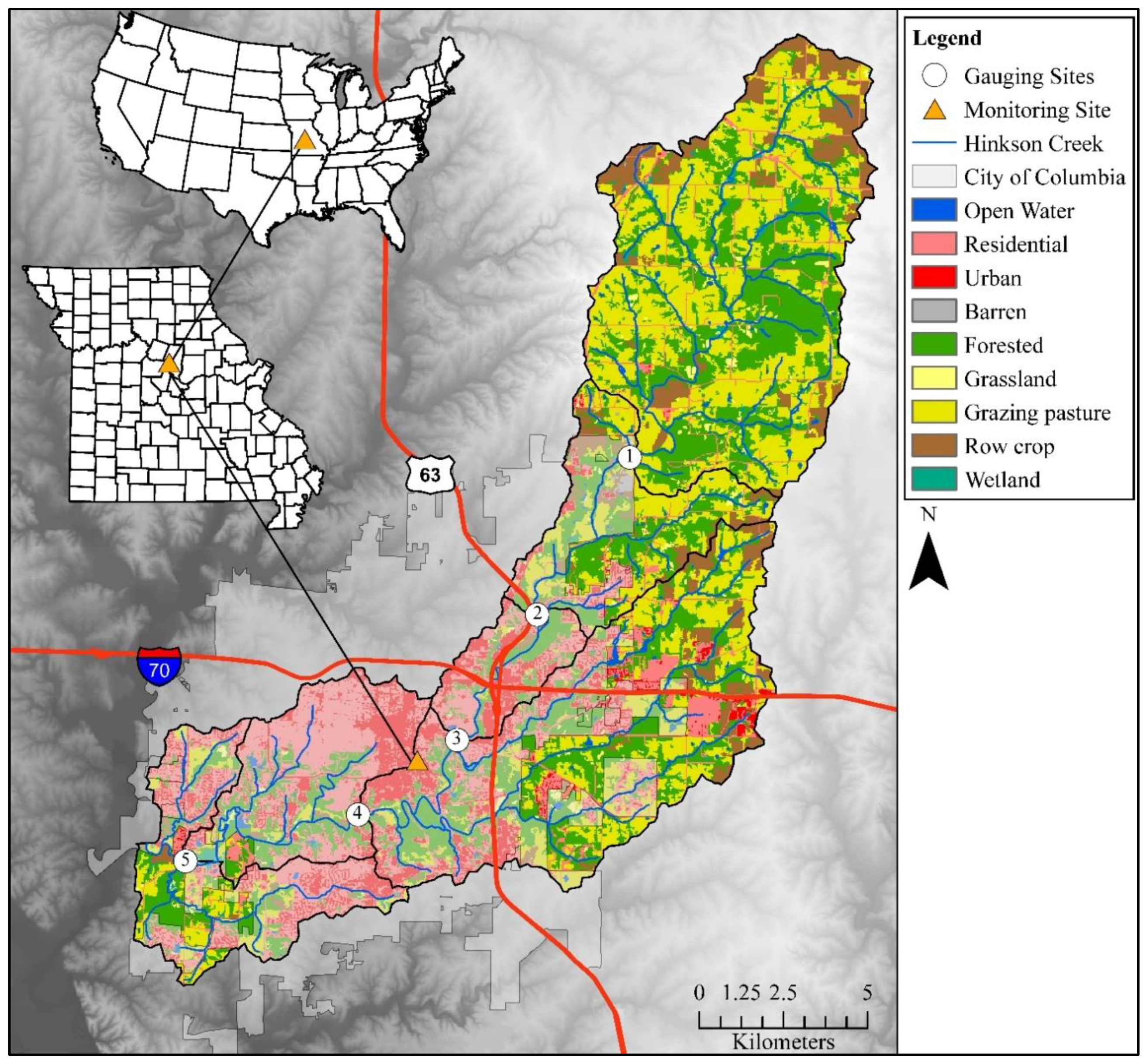
Hinkson Creek Watershed (HCW) is a rapidly urbanizing mixed-land-use (i.e., 33% forested, 38% agricultural, and 26% urban) catchment with an area of approximately 228 km2, located in central MO, USA (Table 1, Figure 1). However, historically (approximately 1800), land cover in HCW was approximately 77% forested/woodland with 21% prairie/savanna, and 2% water/wetland land cover, as indicated using NRCS-USDA ESD and OSD [13,14]. Forested land cover was oak-hickory dominated, agricultural land use was primarily grazing pasture, and urban land use was mainly residential in HCW during this study. Urban land use was associated with approximately 27.7 km2 of impervious surfaces, where the municipal boundary of the City of Columbia (population 113,225 [31,32]) encompassed the lower elevations of the study catchment. Approximate elevations ranged from 274 m above mean sea level (AMSL) in the headwaters to 177 m AMSL at the outlet.
Differences in soils and underlying geology divide HCW near the rural/urban interface. In the agricultural headwaters, clay loam till soils corresponding to the Mexico–Leonard association are underlain by Pennsylvanian sandstone [33,34]. Soils in the headwaters are associated with increased surface runoff potential (hydrologic groups C and D), with infiltration rates as low as 0.001 cm h−1 [35] due to the presence of a well-developed claypan of smectitic minerals found in the argillic (Bt) horizon. Near the watershed outlet, cherty clay solution residuum soils corresponding to the Weller–Bardley–Clinkenbeard (CBC) association are underlain by Burlington formation Mississippian series limestone [30,31]. Hubbart et al. [36] reported alluvial soils with infiltration rates of 126.0 cm h−1 at urban bottomland hardwood forest (BHF) sites, indicating urban BHF sites were well-suited to attenuate urban stormwater runoff and flooding in HCW.
A 30-year climate record (1981–2010) showed average air temperature and annual total precipitation of 13.3 °C and 1176 mm, respectively, in HCW. Air temperatures ranged from −23.1 °C to 41.3 °C [32]. Climate is dominated by continental polar air masses during the winter. Snowfall is common during winter months. A wet season occurs when maritime and continental tropical air masses begin to move back into the region from March through June [32,37].
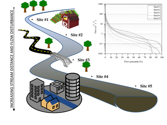
Hinkson Creek, the main channel of HCW, is a storm flow dominated with a base flow index of 0.27 near the watershed outlet [38]. During winter 2008, HCW was instrumented with a nested-scale experimental watershed study design [37]. Five hydroclimate gauging sites were positioned along the main channel to divide HCW into five sub-basins, each with different dominant land uses (Table 1, Figure 1). Sites #1–4 were nested within Site #5, and Site #5 was located near the watershed outlet (Figure 1). Stage and discharge have been intermittently monitored by USGS employees at Site #4 since 1967.
2.2. Data Collection
Climate stations at each gauging site (n = 5) were used to monitor precipitation and stage data used for this research during the study period (water years 2009–2015) (Figure 1). Rainfall was sensed using TE525WS tipping bucket rain gauges with an accuracy of +1% at 2.5 cm h−1 rainfall rate to −3.5% at 5.1–7.6 cm h−1 rainfall rate. Stage was sensed using Sutron Accubar® constant flow bubblers with accuracy of 0.02% at 0–7.6 m to 0.05% at 7.6–15.4 m. Precipitation and stage data were stored on Campbell Scientific CR-1000 data loggers. Methods used to estimate discharge included standards published by Turnipseed and Saur [39]. Stream velocity was measured using FLO-MATE™ Marsh McBirney flow meters and wading rods when stage was less than 1 m deep. Storm flows were measured using a USGS Bridge Board™. Stage–discharge rating curves were generated using the incremental cross-section method to estimate stream flow [40].
2.3. Pre-Settlement SWAT Modeling
Baseline hydrologic conditions of a historic flow regime prior to anthropogenic flow disturbance (i.e., pre-settlement flows) were simulated using SWAT to quantitatively assess the extent of current flow alterations against pre-settlement flows in HCW [5]. The SWAT model was an appropriate choice for the current work, as the model was designed, in part, to simulate streamflow in ungauged sub-basins [13]. Seven water years (2009–2015) of a reference flow regime were simulated using a calibrated SWAT model converted to simulate pre-settlement land cover based on soil physical characteristics in the current work. The duration of the modeling period encompassed the variability of climate, including wet, average, and dry years, as per recommendations from Arnold et al. [13]. The hydrologic data used in this analysis captured the variability of flow, considering flow data were collected across wet (WY2009 and WY2010), average (WY2011, WY2013, and WY2014), and dry (WY2012) years within a 7-year duration.
A previously calibrated and validated SWAT model was used in the current work [41]. The model was calibrated concurrently from Site #1 in the headwaters to Site #5 near the watershed outlet. The autocalibration software SWAT-CUP was used as per methods suggested by Arnold et al. [13,41], with great care to adjust calibration parameters within physically realistic bounds. Model performance was assessed using guidelines published by Moriasi et al. [42,43], generally showing ‘satisfactory’ results in the study catchment following model calibration. Nash–Sutcliffe efficiency values (NSE) were above the guidelines published by Moriasi et al. [42,43] (e.g., streamflow (NSE = 0.83), sediment (NSE = 0.78), total phosphorus (NSE = 0.81), nitrate (NSE = 0.90), and total inorganic nitrogen (NSE = 0.86)). Additional information regarding the calibration methods used, input datasets, model forcings, and model performance results can be found in Zeiger and Hubbart [41].
The calibrated SWAT model was converted to simulate pseudo pre-settlement (approximately 1800) reference conditions, as per recommendations published by Bressiani et al. [44], who suggested calibrating a model prior to land cover conversion to improve model accuracy. Current climate and elevation input data were used as inputs in the pre-settlement SWAT model to focus on the effects of land use and land cover on flow [41]. Climate data were sourced from observed data collected at each nested gauging site in HCW. National Land Cover Dataset (2011) input data were converted to native land cover dependent on soil characteristics using NRCS-USDA ESD and OSD [14,15]. For example, all agricultural and urban areas with ‘Mexico’ soils were converted to native grassland, and areas with ‘Weller’ soils were attributed as forested. Management operations were dependent on native vegetation. For example, native grassland land cover was attributed ‘tall fescue’, and forested land cover was attributed ‘deciduous forest’ cover. Additionally, Soil Conservation Service curve numbers (CN2) and overland roughness (OV_N) parameters were updated to reflect native land cover under ‘good’ conditions using values provided in the USDA Technical Release 55 [45]. The SWAT soil database was updated to convert developed ‘Urban Harvester’ soils to native ‘Weller’ soils in the lower urban reaches of HCW to simulate pre-development soil characteristics important for pre-development flows. All other model parameters were left at default, excepting parameters adjusted during model calibration, as outlined in Zeiger and Hubbart [41].
2.4. Statistical Analysis
A USGS R package EflowStats was downloaded (https://github.com/USGS-R/EflowStats) and used to calculate 171 ‘ecologically relevant’ hydrological indices [5] at each Hinkson Creek (HC) gauging site. A detailed description of the 171 indices included in EflowStats can be found in “Users’ Manual for the Hydroecological Integrity Assessment Process Software” [30]. Initially, EflowStats tools in R were used to download daily flow/peak flow tables and drainage area data from USGS databases. Then, flow data were rewritten using R scripts and daily flow at each HC gauging site. The appropriate drainage area was also updated in R for each HC gauging site. Ultimately, 171 hydrological indices were calculated from two different 7-year daily flow records: (1) simulated pre-settlement (i.e., reference) conditions, and (2) observed current developed conditions at each HC gauging site. Each flow record contained wet, average, and dry water years, considering climate input data included a record-setting wet year (2009) and a year of extreme drought (2012) [41,46]. It was impractical to show results of all 171 hydrologic indices at five sites in a table, thus median and maximum monthly flow magnitude statistics were selected to highlight seasonal differences in flow magnitude due to land use.
Principal component analysis was performed to examine intercorrelation and minimize multicollinearity among the pool of 171 hydrologic indices [5,6]. Using PCA, one primary hydrologic index was selected for each major element of the flow regime, including flow magnitude, frequency, duration, timing, and rate of change across low, average, and high flows, as per methods used by Olden and Poff [6]. A total of nine flow elements were considered in this study, including low, average, and high flow magnitude; low and high flow duration; low and high flow frequency; flow timing; and average rate of change.
An initial PCA was conducted using correlation matrices with pairwise comparisons and two principal components for each flow element (e.g., high flow magnitude, low flow duration, average-flow rate of change) at each HC gauging site [5,6]. Then, broken-stick models were used to select the number of statistically significant principal components as per recommendations by Jackson (1993) [47], where observed eigenvalues from the initial PCA were compared to simulated random eigenvalues generated by broken-stick models [5,6,47]. The number of observed eigenvalues that exceeded broken-stick model-simulated random eigenvalues showed the appropriate number of principal component axes for use in the final PCA [47]. Principal component analysis input parameters were then updated to show the appropriate number of principal components (1–4 in the current work) for each flow element. Results from PCA, in part, showed extracted eigenvectors (i.e., loadings) to each hydrologic index for each principal component axis. Absolute ‘loadings’ were sorted in ascending order to isolate hydrologic indices that explained the most variance along each principal component axis [5,6]. Isolated hydrologic indices for each flow element were used to calculate environmental flow targets at each HC gauging site. Definitions for selected hydrologic indices are presented in Table 2.
3. Results
3.1. Pre-Settlement SWAT Modeling
Observed climate input data included wet, average, and dry years. Annual total precipitation ranged from 669 to 1448 mm during the study (water years 2009–2015). Climate input data also included relatively cold and hot seasonal conditions, with air temperatures that ranged from −28.7 during winter months to 42.8 °C during summer months and an annual mean air temperature of 14.1 °C. Observed total solar ranged from 0.5 to 29.5 MJ m−2 with a mean of 13.5 MJ m−2. It is important to note that current hydroclimate inputs were used in pre-settlement SWAT model simulations, thus, any alterations to the daily flow were due to changes linked to LULC and management operations.
Pre-settlement simulated mean daily stream flow was slightly greater than the current observed stream flow by 0.2 m3 s−1 at a USGS-monitored gauging site (Site #4) located in the lower urbanized reaches of Hinkson Creek Watershed (Table 3). Simulated pre-settlement median daily stream flow was 0.8 m3 s−1 greater than that observed flow at Site #4 (Table 3). Also, maximum daily flow decreased by 22.0 m3 s−1. Minimum daily flow was less than 0.1 m3 s−1 for simulated and observed flow regimes, and flow variability decreased by 2.7 m3 s−1. Thus, it was evident that maximum daily flow increased, while steady flows decreased between pre-settlement and developed periods, respectively, at Site #4 in the study catchment.
3.2. Statistical Analysis
It was important to show differences in mean and median flow magnitude statistics at each gauging site to highlight potential effects of developed land use on average and high flow magnitude evident from this study. Results showed simulated pre-settlement median monthly flow (MA12–23) was ±0.2 m3 s−1 compared to observed developed flow during the first quarter (January–March), except at urban Sites #4 and #5 during March, when the developed median monthly flow was 0.4 m3 s−1 greater than pre-settlement conditions (Table 4). Simulated pre-settlement median monthly flow was consistently greater than observed flow by 0.2–1.9 m3 s−1 at all sites during the remaining quarters and months of the year (Table 4). These results highlight the potential for developed land use to decrease median flows in the study catchment.
Simulated pre-settlement median maximum monthly flow (MH1–12) was within ±16.0 m3 s−1 compared to observed developed flow during the first, third, and fourth quarters of the study (Table 5). However, pre-settlement median maximum flow was generally less than observed during the second quarter, especially during April, when pre-settlement median maximum monthly flows were 21.3–78.5 m3 s−1 less than developed conditions at Sites #1–5 (Table 5). These results show the potential for developed land use to increase maximum flows, especially during wet months, in the study catchment.
Results from the initial PCA showed substantial intercorrelation between selected hydrologic indices. For example, the first principal component (PC1) (i.e., ordination results that spanned the direction of the most variation in hydrologic indices) explained 39–66% of the variance in each flow element (e.g., high flow magnitude, low flow duration, etc.), and eigenvalues ranged from 1.8 to 28.3. The second principal component (PC2) (i.e., ordination results that spanned the direction of the second most variation in hydrologic indices) explained 66–92% of the cumulative variance in flow indices, and eigenvalues ranged from 0.9 to 8.3.
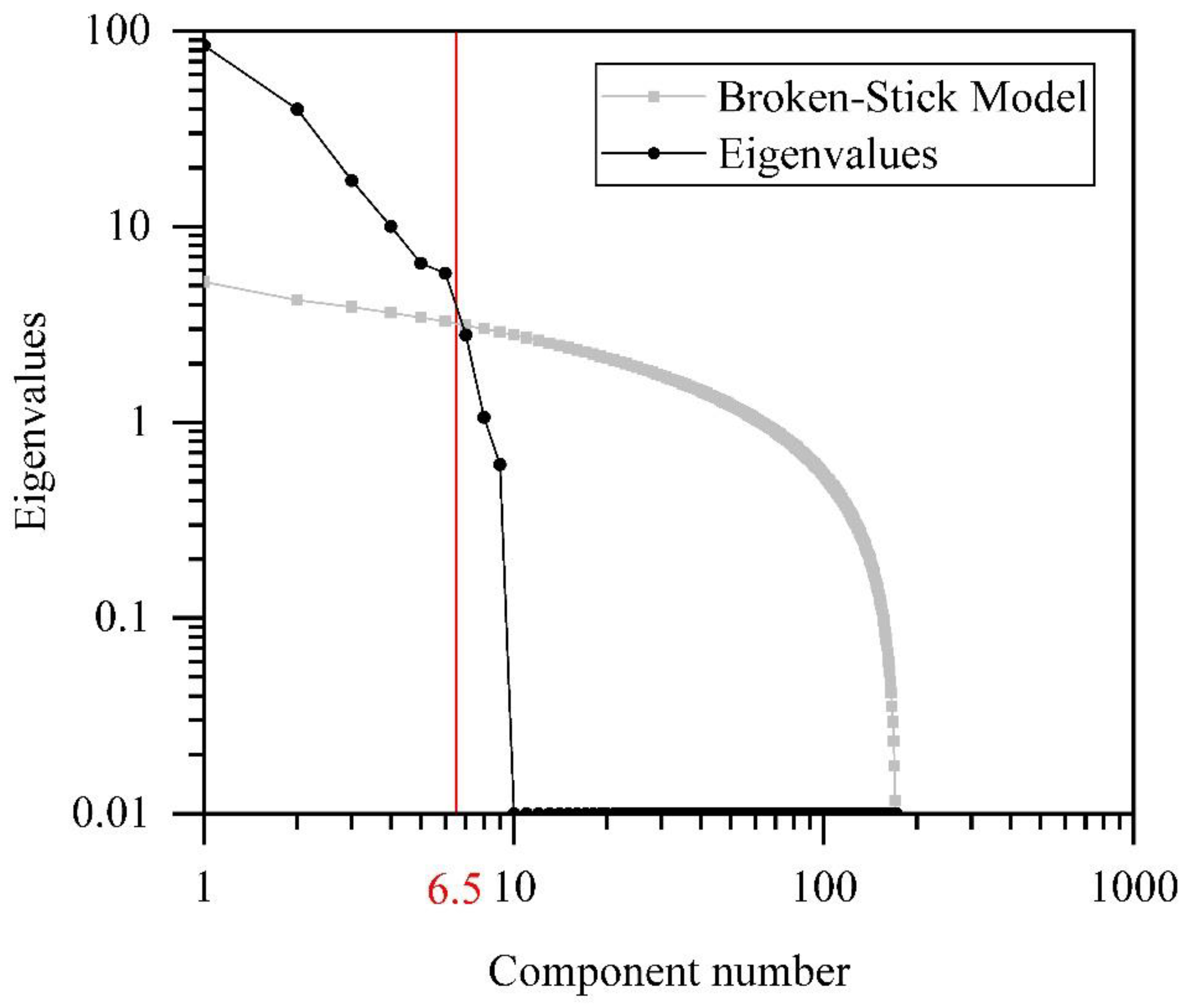
Broken-stick models were used to indicate the number of statistically significant principal components to consider, ranging from 2 to 3 (Table 6, Figure 2). The number of principal component axes were updated to reflect results from broken-stick model analysis and PCA results were updated. Results from PCA indicated the nine flow statistics with the greatest absolute loadings that explained the most variation of 171 hydrologic indices across all major elements of a flow regime in the study catchment. Results showed greatest absolute loadings of PC1 ranged from 0.187 (average flow magnitude) to 0.688 (low flow frequency) (Table 6). Thus, the subset of nine indices were high-information non-redundant hydrologic indices in the study catchment. Selected indices with the greatest absolute loadings on PC1 were exported for further analysis to quantify environmental flow targets in the study catchment. However, the indices from PC2 and PC3 axes (shown in Table 5) are also deemed important in Hinkson Creek, and stream types of the region similar to principal component axes were orthogonal by definition, and thus, independent.
3.3. Environmental Flow Targets
Results showed high flow volume (MH22) ranged from 18.2 to 22.6 days (pre-settlement) and from 113.6 to 220.1 days (developed) (Table 7). High flow frequency (FH6) ranged from 12 to 19 events per year (pre-settlement) and from 16 to 22 events per year (developed). The trend for developed FH6 values to increase by six events per year over 30.2 km stream length was exacerbated by urban land use during developed conditions. These results indicated simulated pre-settlement high flow magnitude, frequency, and duration were substantially lower compared to the observed developed flow in the study catchment.
Simulated pre-settlement low flow statistics were usually higher than developed low flows (Table 7). Variability in base flow (ML18) ranged from 174 to 188% (pre-settlement) and from 46 to 83% (developed). Low flood pulse counts (FL1) ranged from 7 to 16 events per year (pre-settlement) and from 6 to 14 events per year (developed). Variability in annual minimum ranged from 209 to 220% (pre-settlement) and from 92 to 145% (developed).
Flow predictability (TA2) values were not substantially different between pre-development and developed flow regimes. However, results showed land use influence on the average Julian date of minimum (TL1) and maximum (TH1) annual flows. Minimum annual flows (TL1) occurred during December and January during pre-settlement conditions and November during developed conditions (Table 7). These results, in concert with other low flow statistics, indicated pre-settlement land use was associated with increased recharge of shallow subsurface storage and subsequent release of baseflow to Hinkson Creek, thereby extending the time to dry season minimum flows (i.e., low flow). Pre-settlement variability in fall rate statistics (RA4), ranging from 282 to 349%, also indicated decreased hydrograph recession in comparison to developed flows (RA4 = 447–617%).
Results from high flow timing statistics showed TH1 occurred on dates ranging from late July (Sites #1, #2, and #5) to early October (Sites #3 and #4). Conversely, observed flow data showed average annual flow maximum occurred from late April to May. October daily rainfall totals can exceed rainfall totals observed during April and May in HCW. However, monthly rainfall totals are generally greater during April and May compared to October. Thus, the pre-settlement average Julian date of annual maximum flows (TH1) was influenced by large rainfall events that occurred during the spring and October in HCW.
4. Discussion
4.1. Pre-Settlement SWAT Modeling
Representative paired catchment investigations with a reference catchment for control are well-suited for developing environmental flow targets. However, paired catchment opportunities often do not exist. While univariate hydrologic–biologic empirical relationships can be useful to generate environmental flow targets, the influence of catchment characteristics (e.g., climate, geology, geomorphology, soils, land use, and management operations) on flow must be considered when assessing environmental flows, as noted by Booker et al. [48]. In the current work, influences of catchment characteristics on flow were accounted for using SWAT. Results show that process-based watershed-scale continuous time models like SWAT can be useful tools for simulating a pre-settlement flow regime. Thus, calls from the literature for rapid, broad-scale environmental flow assessments [2] can be answered using physical hydrologic models like SWAT.
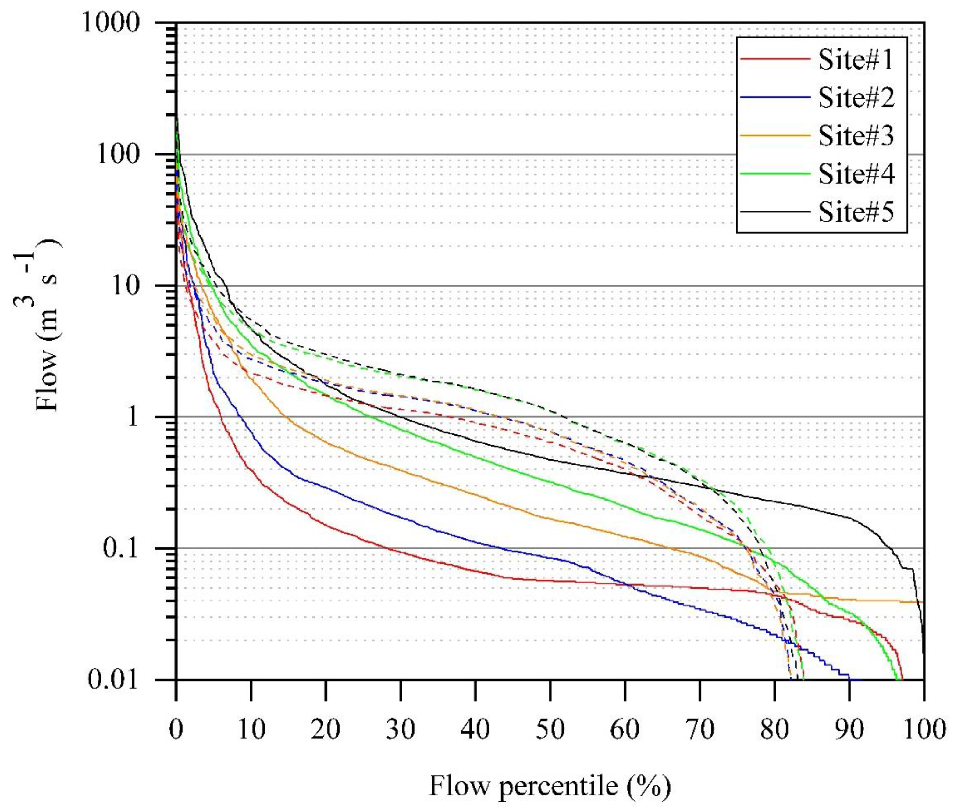
The trend for increased high flows and decreased steady flows between pre-settlement and developed periods in the study catchment was apparent when flow duration curves were plotted for visual comparison (Figure 3). Pre-settlement simulated median daily stream flow increased by 0.8 m3 s−1 compared to observed flow at a USGS-monitored gauging site (Site #4) located in the lower urbanized reaches of Hinkson Creek Watershed. The percent difference in median daily stream flow was about 115% between pre-settlement and developed conditions. Also, maximum daily flow decreased by approximately 13%, with a 34% decrease in daily flow variability. This science-based information may be important for management regionally, and also shows the potential for land use impacts in similar developed watersheds globally.
4.2. Statistical Analysis
Olden and Poff [6] noted that the hydrologic indices included in the R statistical package EflowStats are ecologically relevant. While the ecological relevance for the initial 171 indices has been well documented, results from this study show potential issues with the timing variables that calculate average Julian date of annual minimum (TL1) and maximum (TH1) flows when more than one wet season occurs. Results from this study show the importance of closely examining each hydrologic index for appropriateness in the area of interest before all 171 indices are reduced using PCA.
When results from EflowStats were analyzed in this study, hydrologic indices dependent on drainage area were area-normalized before being used as inputs in PCA. Unfortunately, normalizing those daily flow data removed much of the variability important in the selection of dominant indices for each principal component axes in PCA, similar to results reported by Kennen et al. [5]. Due to this issue, some flow magnitude indices (currently 38 of 171 indices) were less likely to be selected for environmental flow targets using PCA. If observed data show certain hydrologic indices are physically important in the study catchment (e.g., median flow magnitude), but were not selected using PCA, it may be appropriate for management to consider those indices for ecological importance in the watershed of interest.
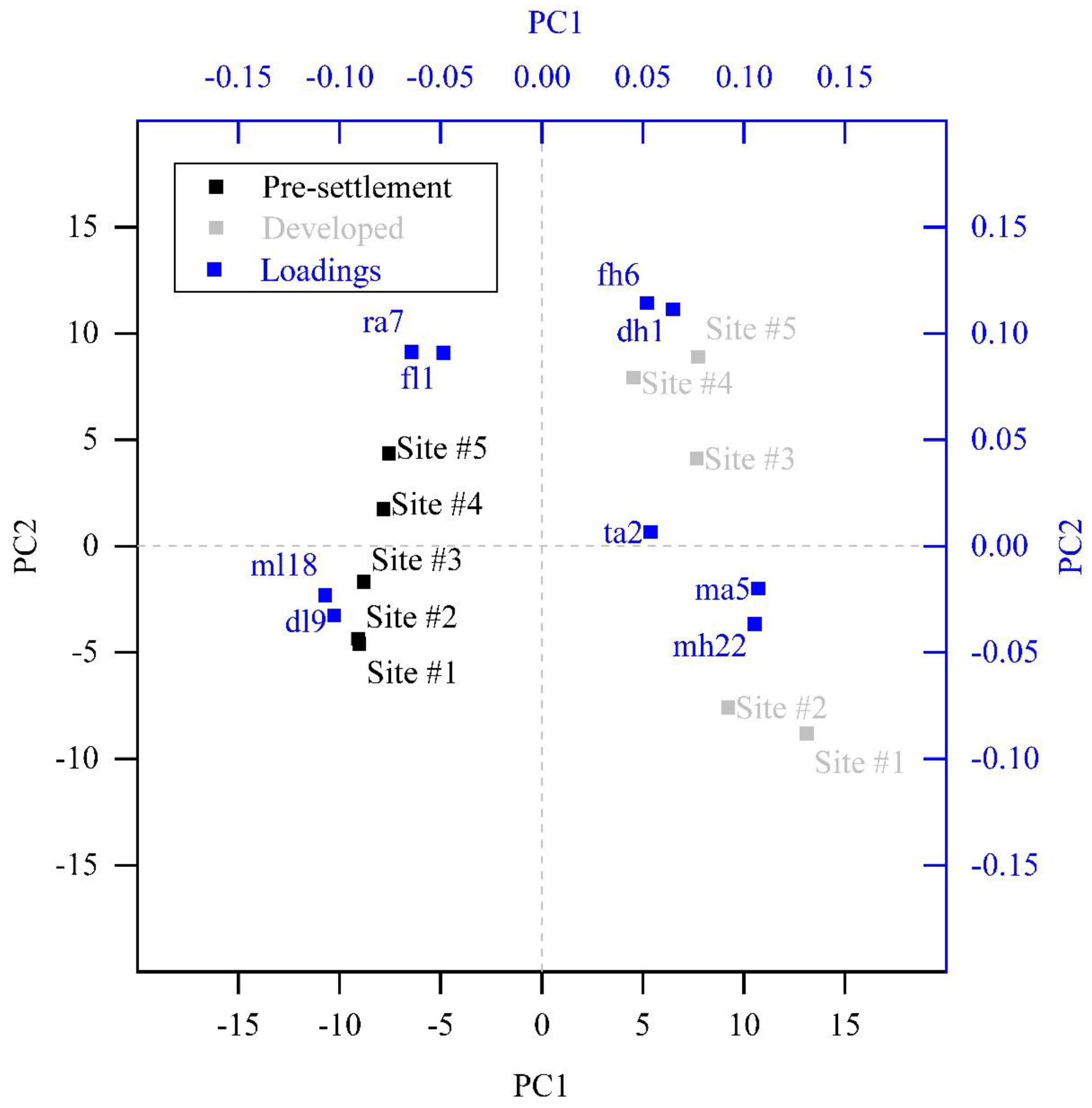
In this study, it was important to analyze the deviation between baseline and current flows (step 3 of ELOHA) to select hydrologic indices best-suited for environmental flow targets. A biplot clearly showed a separation of baseline and developed flows along the first principal component axis (PC1), with pre-settlement flows clustered on the left and developed sites to the right (Figure 4). Additionally, there was a clear separation of rural and urban sites along the second principal component axis, highlighting urban land use alteration to developed flows, with urban sites above the origin and rural sites below it. Only the hydrologic indices with the greatest absolute loadings for each major element of the flow regime were shown in the biplot, as 171 clustered indices made it difficult to interoperate key findings. Indices with the greatest absolute distance from the origin in the biplot explained the most variability in the group of 171 indices. These results indicated the potential benefits of including baseline and current flow data in PCA for selecting hydrologic indices altered by human activity.
Flow predictability (TA2) was less important than the other indices shown in the biplot, which may be reasonable considering the percent differences of TA2 ranged from less than 1 to 16% between pre-developed and developed flows. Conversely, flood frequency (FH6) loadings were relatively large, with percent differences ranging from 10 to 29% between pre-settlement and developed flows. Flow magnitude statistics were also important, with percent differences ranging from −78% (low flow magnitude (ML18)) to 169% (high flow magnitude (MH22)). These results show how including baseline and developed flows in PCA is a superior method for selecting hydrologic indices most important for determining the deviation between baseline and current flow conditions (step 3 of ELOAH). Step 4 of ELOHA has not been conducted for streams of Missouri, including Hinkson Creek, however, step 4 is implied [5], assuming pre-settlement flows once supported healthy aquatic ecosystems.
Previous studies have performed PCA using observed baseline flows from relatively undisturbed streams to separate stream types in a region (step 2 of ELOHA) [5,6]. Streams with flow alteration, catchment urbanization, poor flow records, or drainage areas greater than 5000 km2 were not included in those analyses. The PCA results grouped reference sites according to stream type, showing how PCA tools were excellent for classifying stream types to reference streams that do not exhibit extensive hydrologic alteration from flow regulation or urbanization. However, hydrologic indices selected from PCA of reference streams may not be the most important environmental flow targets in streams that exhibit hydrologic alteration due to urban land use, like Hinkson Creek. It is important to consider that PCA is a statistical test, and thus, results from regional PCA should be carefully examined to ensure physically meaningful indices are selected for environmental flow targets at the watershed scale.
Selecting environmental flow targets based on eigenvalues with the greatest absolute loadings is problematic when selected targets are not causally linked to flow alteration in the stream or river of interest. The magnitude, frequency, and duration of high flow indices selected using PCA in the current work were different from Kennen et al. [5]. For example, flood frequency (FH6) was not associated with the greatest absolute loadings in flashy/runoff dominated streams of Missouri by Kennen et al. [5], unlike this study. The lack of significant differences indicated that those indices were irrelevant for flow management in HCW at the time of this study. That is not to suggest that those facets of the flow regime are not important for flow management in HCW. Further, that is not to say flows are unaltered in Hinkson Creek. What these results do suggest is that flow management efforts may be ineffective when based on PCA results from regional assessments, at least in part, due to variability in watershed characteristics and anthropogenic activity within stream types, but also due to results from statistical analysis generated using only reference sites without hydrologic alteration from flow regulation or catchment urbanization.
4.3. Environmental Flow Targets
The importance of flow in shaping aquatic communities is globally accepted [17,49,50]. For example, Hughes and James [17] showed discharge (Q) influence on aquatic plant community structure and dynamics in perennial flashy and perennial runoff stream types with drainage areas that ranged from 36.4 to 448 km2. Low (Q < 0.1 m3 s−1), steady (0.1 < Q < 50 m3 s−1), and high (Q > 50 m3 s−1) flow events were significantly correlated (F-values > 2.77; p < 0.1) with aquatic plant cover in addition to species richness, diversity, turnover, and evenness [17]. Thus, results from previous literature highlight the potential ecological implications of land use-induced flow alteration observed in Hinkson Creek [17,25,49,50].
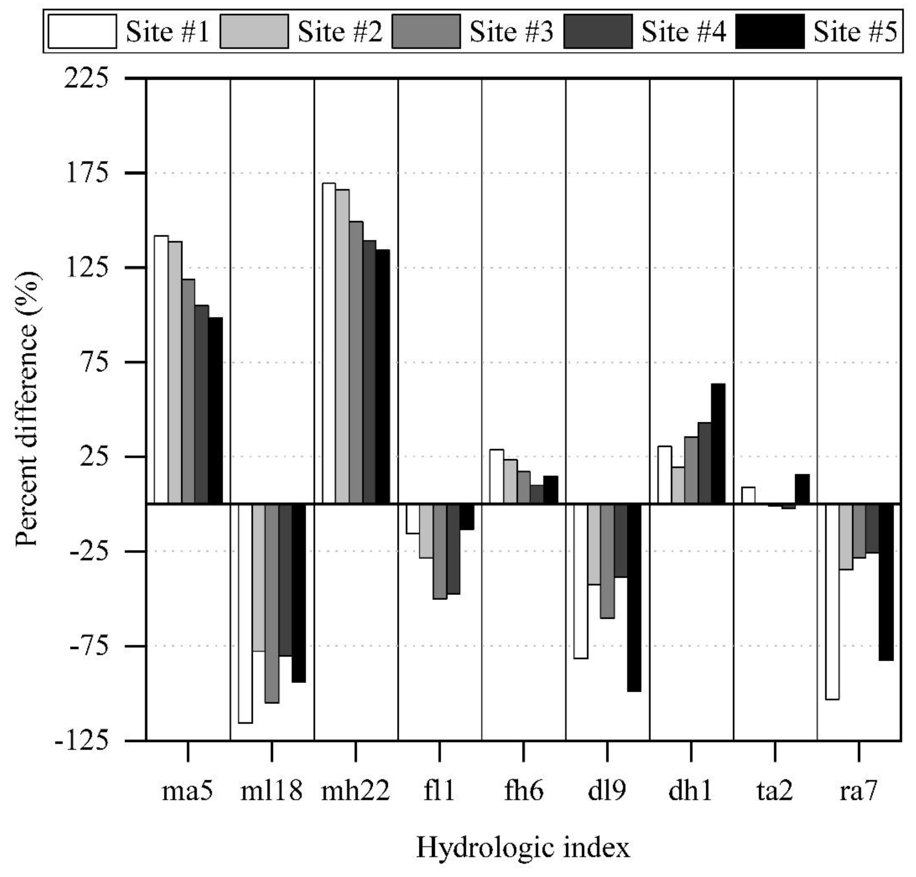
Results showed alterations to flow were evident across every major element of the flow regime at each of the five gauging sites on Hinkson Creek, especially flow magnitude. For example, high flow volume (MH22) was 84–169% greater during developed flows compared to pre-settlement flows. Skewness (MA5) is also an indicator of increased high flow volume (Figure 5). Results showed percent differences in MA5 ranged from 98 to 142% between current flows and pre-settlement flows at the five gauging sites. That is not to suggest that flow magnitude has greater environmental implications relative to other elements of the flow regime, like flow frequency.
High flow frequency (FH3), defined as the average number of days flows are above 3 times the median flow per year, was nearly equal, by definition, to FH6, defined as the average number of events above 3 times the median flow per year. Index FH3 was selected as “the most ecological useful overall flow variable” of 34 hydrologic variables tested when FH3 explained the most variance in many benthic community measures tested by Clausen and Biggs [25]. High flow frequency has been linked to a mechanistic control on biota, in agreement with stream ecosystem theory [25]. In the current work, FH3 was 41–76% higher for current conditions compared to pre-settlement conditions, generally increasing with drainage area from rural Site #1 to urban Site #4 (Figure 3). Further, FH3 was substantially greater by 26–48% at urban sites relative to rural sites. Thus, the trend for developed FH3 values to increase with drainage area was exacerbated by urban land use coverage commensurate with a classic mechanistic understanding of impervious surface influence to high flow frequency [7]. The environmental implications for increased high flow frequency, taken from Clausen and Biggs [25], shows the potential for decreased periphyton biomass, species richness, and diversity, especially at urban sites. Further research is needed to quantify direct linkages between ecologically relevant flow indices selected in the current work and observed ecological communities in the study catchment.
Such substantial deviations between observed developed flows and simulated pre-settlement flows indicate potential benefits for environmental flow restoration efforts in HCW and similar mixed-land-use watersheds. However, restoration of the historic flow regime prior to European settlement may not be practical where watershed characteristics have been substantially altered by land use. In the current work, land cover conversion to pre-settlement watershed characteristics resulted in increased infiltration, shallow groundwater recharge, and baseflow coupled to decreased high flow volume and high flow frequency. There are engineering practices that can increase retention and infiltration of excessive runoff in developed catchments by diverting excessive runoff to naturally occurring near-surface valley bottom storage (e.g., bottomlands, wetlands, bank soils, and alluvial fills). However, infiltration techniques alone are unlikely to result in flow regime restoration, where urban land use has dramatically altered evapotranspiration rates [7,51]. Results from previous studies show the potential benefits of infiltration techniques coupled to additional water harvesting for uses like landscape irrigation to restore flow regimes in developed catchments [7,51].
4.4. Study Implications and Future Work
Environmental flow recommendations set to protect a specific fish, macro-invertebrate, or algal population may not account for total aquatic ecosystem health [4]. Alternatively, environmental flow targets developed in this study aim to restore a historic flow regime, and thus promote total ecosystem health. An important assumption is that the historic flow regime once supported a heathy ecosystem. It is also important to note that restoration of a historic flow regime may not be achievable in contemporary watersheds where climate change and human activity (past and present) have extensively altered overland watershed characteristics, channel geomorphology, and water quality.
Results from this study show environmental flow targets are necessary to mitigate ecological degradation due to rapid human development (particularly urbanization) in agreement with previous works [7,8]. The environmental flow targets quantified in the current work could be used to help guide local managers interested in restoring flows prior to land use development in the study catchment. In general, results show high flow magnitude and frequency should be reduced. Thus, future agricultural and urban land use and management operations that increase surface runoff and velocity should be balanced with restoration efforts to avoid exacerbating environmental flow alteration in HCW.
There is a need to consider environmental flow targets appropriate for watersheds already modified by existing land use similar to HCW. The underlying assumption that flow management will lead to improved water quality needs to be validated. Thus, future research is needed to confirm that the environmental flow recommendations from this study and similar regional assessments are: (1) realistically achievable, and (2) appropriate for mitigation strategies implemented to improve water quality (e.g., stream temperature, suspended sediment, nutrient regimes) and total aquatic ecosystem health.
The SWAT model is an attractive choice for simulating baseline flow conditions when observed data are not available. Model development has substantially increased model accuracy and reduced model limitations over the past decades. However, uncalibrated SWAT model simulations of daily flow should be examined carefully before being used to develop environmental flow standards. When possible, it is beneficial to calibrate SWAT to the variable of interest (in this case flow) prior to land cover conversion for simulating baseline flow conditions [41]. Great care should be taken to keep model parameters physically realistic during model calibration [13]. Overall, results from this study show that a calibrated SWAT model can be used to simulate baseline conditions when observed baseline flow data are not available. More modeling research and development are necessary to test the efficacy of using an uncalibrated SWAT model to simulate daily environmental flow targets. If uncalibrated modeling results are unsatisfactory, then calibrated model results can be scaled up from instrumented representative watersheds to nearby watersheds with similar characteristics. Results from this study indicate the usefulness of process-based modeling tools in concert with statistical methods to develop watershed-scale environmental flow targets based on historic flow regimes.
5. Conclusions
Rapid urbanization and agricultural development have altered environmental flow regimes globally. The pace of impairment exceeds management efforts to mitigate flow alteration. Regional efforts based on standardized methodologies (e.g., ELOHA and HIP) are needed to assess environmental flows. The overarching objective of the current work was to assess the efficacy of environmental flow targets based on SWAT-simulated pre-settlement flows in a contemporary mixed-land-use catchment (i.e., urban, agricultural, and forested).
Results showed land use impacts to each major facet of the flow regime in the study catchment, especially during high flows. Average and high flow magnitude (MA5 and MH22) increased by 98–169%, between baseline and current flows. Land use-related alterations to the median maximum flow magnitude were apparent, especially during wet months (April–June), with percent differences of 74–101% during April. Ecologically relevant flow frequency statistics, including high flow frequency (FH3) and flood frequency (FH6), increased by 45–76% and 10–29%, respectively, between baseline and current flows. Thus, key findings from this study generally show that environmental flow recommendations should result in decreased high flow magnitude and frequency. This science-based information shows the potential for extensive alterations to high flows in similar mixed-land-use watersheds globally. Results indicate that environmental flow targets dependent on a historic flow regime may not be socioeconomically practical in watersheds already extensively altered by past and present agricultural and urban land uses. Ultimately, there will be a need to achieve a balance between desired land use and environmental flow targets as human activity continues to alter flows in the study catchment and similar mixed-land-use watersheds globally.
Author Contributions
Data curation, S.Z.; Formal analysis, S.Z.; Funding acquisition, J.H.; Project administration, J.H.; Writing—original draft, S.Z.; Writing—review & editing, J.H.
Funding
This research was funded by the Missouri Department of Conservation and the U.S. Environmental Protection Agency Region 7 through the Missouri Department of Natural Resources (P.N: G08-NPS-17) under Section 319 of the Clean Water Act and through joint agreement of the University of Missouri, the City of Columbia, and Boone County Public works and partners of the Hinkson Creek Collaborative Adaptive Management (CAM) program. Additional funding was provided by the National Science Foundation under Award Number OIA-1458952, the USDA National Institute of Food and Agriculture, Hatch project accession number 1011536, and the West Virginia Agricultural and Forestry Experiment Station. Results presented may not reflect the views of the sponsors and no official endorsement should be inferred.
Acknowledgments
Special thanks are due to many scientists of the Interdisciplinary Hydrology Laboratory (www.forh2o.net).
Conflicts of Interest
The authors declare no conflict of interest.
References
- Arthington, A.H.; Bunn, S.E.; Poff, N.L.; Naiman, R.J. The challenge of providing environmental flow rules to sustain river ecosystems. Ecol. Appl. 2006, 16, 1311–1318. [Google Scholar] [CrossRef]
- Poff, N.L.; Zimmerman, J.K. Ecological responses to altered flow regimes: A literature review to inform the science and management of environmental flows. Freshw. Biol. 2010, 55, 194–205. [Google Scholar] [CrossRef]
- Acreman, M.C.; Dunbar, M.J. Defining environmental river flow requirements? A review. Hydrol. Earth Syst. Sci. Discuss. 2004, 8, 861–876. [Google Scholar] [CrossRef]
- Poff, N.L.; Richter, B.D.; Arthington, A.H.; Bunn, S.E.; Naiman, R.J.; Kendy, E.; Henriksen, J. The ecological limits of hydrologic alteration (ELOHA): A new framework for developing regional environmental flow standards. Freshw. Biol. 2010, 55, 147–170. [Google Scholar] [CrossRef]
- Kennen, J.G.; Henriksen, J.A.; Heasley, J.; Cade, B.S.; Terrell, J.W. Application of the Hydroecological Integrity Assessment Process for Missouri Streams; USGS: Fort Collins, CO, USA, 2009.
- Olden, J.D.; Poff, N.L. Redundancy and the choice of hydrologic indices for characterizing streamflow regimes. River Res. Appl. 2003, 19, 101–121. [Google Scholar] [CrossRef]
- Walsh, C.J.; Fletcher, T.D.; Burns, M.J. Urban stormwater runoff: A new class of environmental flow problem. PLoS ONE 2012, 7, e45814. [Google Scholar] [CrossRef] [PubMed]
- Fletcher, T.D.; Mitchell, V.; Deletic, A.; Ladson, T.R.; Seven, A. Is stormwater harvesting beneficial to urban waterway environmental flows? Water Sci. Technol. 2007, 55, 265–272. [Google Scholar] [CrossRef] [PubMed]
- Carlisle, D.M.; Wolock, D.M.; Meador, M.R. Alteration of streamflow magnitudes and potential ecological consequences: A multiregional assessment. Front. Ecol. Environ. 2010, 9, 264–270. [Google Scholar] [CrossRef]
- Poff, N.L.; Allan, J.D.; Bain, M.B.; Karr, J.R.; Prestegaard, K.L.; Richter, B.D.; Stromberg, J.C. The natural flow regime. BioScience 1997, 47, 769–784. [Google Scholar] [CrossRef]
- Pastor, A.V.; Ludwig, F.; Biemans, H.; Hoff, H.; Kabat, P. Accounting for environmental flow requirements in global water assessments. Hydrol. Earth Syst. Sci. 2014, 18, 5041–5059. [Google Scholar] [CrossRef] [Green Version]
- Arthington, Á.H.; Naiman, R.J.; McClain, M.E.; Nilsson, C. Preserving the biodiversity and ecological services of rivers: New challenges and research opportunities. Freshw. Biol. 2010, 55, 1–16. [Google Scholar] [CrossRef]
- Arnold, J.G.; Moriasi, D.N.; Gassman, P.W.; Abbaspour, K.C.; White, M.J.; Srinivasan, R.; Santhi, C.; Harmel, R.D.; van Griensven, A.; Van Liew, M.W.; et al. SWAT: Model use, calibration, and validation. Am. Soc. Agric. Biol. Eng. 2012, 55, 1491–1508. [Google Scholar]
- U.S. Department of Agriculture, Natural Resources Conservation Service (USDA-NRCS). National Soil Survey Handbook, Title 430-VI. Available online: http://www.nrcs.usda.gov/wps/portal/nrcs/detail/soils/ref/?cid=nrcs142p2_054242 (accessed on 6 June 2018).
- U.S. Department of Agriculture, Natural Resources Conservation Service (USDA-NRCS). Ecological Site Descriptions. Available online: https://esis.sc.egov.usda.gov/Welcome/pgESDWelcome.aspx (accessed on 6 June 2018).
- Archfield, S.A.; Kennen, J.G.; Carlisle, D.M.; Wolock, D.M. An objective and parsimonious approach for classifying natural flow regimes at a continental scale. River Res. Appl. 2014, 30, 1166–1183. [Google Scholar] [CrossRef]
- Hughes, J.M.R.; James, B. A hydrological regionalization of streams in Victoria, Australia, with implication for stream ecology. Aust. J. Mar. Freshw. Res. 1989, 40, 303–326. [Google Scholar] [CrossRef]
- Poff, N.L.; Ward, J.V. Implications of streamflow variability and predictability for lotic community structure—A regional analysis of streamflow patterns. Can. J. Fish. Aquat. Sci. 1989, 46, 1805–1818. [Google Scholar] [CrossRef]
- Richards, R.P. Measures of flow variability for Great Lakes tributaries. Environ. Monit. Assess. 1989, 12, 361–377. [Google Scholar] [CrossRef] [PubMed]
- Richards, R.P. Measures of flow variability and a new flow-based classification of Great Lakes tributaries. J. Great Lakes Res. 1990, 16, 53–70. [Google Scholar] [CrossRef]
- Poff, N.L. A hydrogeography of unregulated streams in the United States and an examination of scale-dependence in some hydrological de-scriptors. Freshw. Biol. 1996, 36, 71–91. [Google Scholar] [CrossRef]
- Richter, B.D.; Baumgartner, J.V.; Powell, J.; Braun, D.P. A method for assessing hydrologic alteration within ecosystems. Conserv. Biol. 1996, 10, 1163–1174. [Google Scholar] [CrossRef]
- Richter, B.D.; Baumgartner, J.V.; Wigington, R.; Braun, D.P. How much water does a river need? Freshw. Biol. 1997, 37, 231–249. [Google Scholar] [CrossRef]
- Richter, B.D.; Baumgartner, J.V.; Braun, D.P.; Powell, J.A. spatial assessment of hydrologic alteration within a river network. Regul. Rivers Res. Manag. 1998, 14, 329–340. [Google Scholar] [CrossRef]
- Clausen, B.; Biggs, B.J.F. Relation-ships between benthic biota and hydrological indices in New Zealand streams. Freshw. Biol. 1997, 38, 327–342. [Google Scholar] [CrossRef]
- Clausen, B.; Biggs, B.J.F. Flow indices for ecological studies in temperate streams: Groupings based on covariance. J. Hydrol. 2000, 237, 184–197. [Google Scholar] [CrossRef]
- Puckridge, J.T.; Sheldon, F.; Walker, K.F.; Boulton, A.J. Flow variability and the ecology of large rivers. Mar. Freshw. Res. 1998, 49, 55–72. [Google Scholar] [CrossRef]
- Clausen, B.; Iversen, H.L.; Ovesen, N.B. Ecological flow indices for Danish streams. In Proceedings of the Nordic Hydrological Conference 2000, Uppsala, Sweden, 26–30 June 2000; pp. 3–10. [Google Scholar]
- Wood, P.J.; Agnew, M.D.; Petts, G.E. Flow variations and macroinvertebrate community responses in a small groundwater-dominated stream in south-east England. Hydrol. Process. 2000, 14, 3133–3147. [Google Scholar] [CrossRef]
- Henriksen, J.A.; Heasley, J.; Kennen, J.G.; Nieswand, S. Users’ Manual for the Hydroecological Integrity Assessment Process Software (Including the New Jersey Assessment Tools); U. S. Geological Survey: Menlo Park, CA, USA, 2006.
- United States Census Bureau (USCB). U.S. Census Bureau: State and County Quick Facts. Available online: http://quickfacts.census.gov/qfd/states/29000.html (accessed on 31 May 2014).
- Hubbart, J.A.; Kellner, E.; Lynne, H.; Lupo, A.R.; Market, P.S.; Guinan, P.E.; Stephan, K.; Fox, N.I.; Svoma, B.M. Localized climate and surface energy flux alterations across an urban gradient in the central US. Energies 2014, 7, 1770–1791. [Google Scholar] [CrossRef]
- Miller, D.E.; Vandike, J.E. Groundwater Resources of Missouri; Missouri Department of Natural Resources, Division of Geology and Land Survey: Rolla, MO, USA, 1997; Volume 2.
- Hubbart, J.A.; Zell, C. Considering streamflow trend analyses uncertainty in urbanizing watersheds: A baseflow case study in the central United States. Earth Interact. 2013, 17, 1–28. [Google Scholar] [CrossRef]
- Blanco-Canqui, H.; Gantzer, C.J.; Anderson, S.H.; Alberts, E.E.; Ghidey, F. Saturated hydraulic conductivity and its impact on simulated runoff for claypan soils. Soil Sci. Soc. Am. J. 2002, 66, 1596–1602. [Google Scholar] [CrossRef]
- Hubbart, J.A.; Muzika, R.-M.; Huang, D.; Robinson, A. Improving Quantitative Understanding of Bottomland Hardwood Forest Influence on Soil Water Consumption in an Urban Floodplain. Watershed Sci. Bull. 2011, 3, 34–43. [Google Scholar]
- Hubbart, J.A.; Holmes, J.; Bowman, G. Integrating science-based decision making and TMDL allocations in urbanizing watersheds. Watershed Sci. Bull. 2010, 1, 19–24. [Google Scholar]
- Zeiger, S.J.; Hubbart, J.A. Nested-Scale Nutrient Yields from a Mixed-Land-Use Urbanizing Watershed. Hydrol. Process. 2015, 30, 1475–1490. [Google Scholar] [CrossRef]
- Turnipseed, D.P.; Sauer, V.B. Discharge Measurements at Gaging Stations (No. 3-A8); US Geological Survey: Menlo Park, CA, USA, 2010.
- Dottori, F.; Martina, M.L.V.; Todini, E. A dynamic rating curve approach to indirect discharge measurement. Hydrol. Earth Syst. Sci. 2009, 13, 847–863. [Google Scholar] [CrossRef] [Green Version]
- Zeiger, S.J.; Hubbart, J.A. A SWAT model validation of nested-scale contemporaneous stream flow, suspended sediment and nutrients from a multiple-land-use watershed of the central USA. Sci. Total Environ. 2016, 572, 232–243. [Google Scholar] [CrossRef] [PubMed]
- Moriasi, D.N.; Arnold, J.G.; Van Liew, M.W.; Bingner, R.L.; Harmel, R.D.; Veith, T.L. Model evaluation guidelines for systematic quantification of accuracy in watershed simulations. Trans. ASABE 2007, 50, 885–900. [Google Scholar] [CrossRef]
- Moriasi, D.N.; Gitau, M.W.; Pai, N.; Daggupati, P. Hydrologic and water quality models: Performance measures and evaluation criteria. Trans. ASABE 2015, 58, 1763–1785. [Google Scholar] [CrossRef]
- Bressiani, D.; Gassman, P.W.; Fernandes, J.G.; Garbossa, L.H.P.; Srinivasan, R.; Bonumá, N.B.; Mendiondo, E.M. Review of soil and water assessment tool (SWAT) applications in Brazil: Challenges and prospects. Int. J. Agric. Boil. Eng. 2015, 8, 9–35. [Google Scholar]
- United States Department of Agriculture (USDA). Urban Hydrology for Small Watersheds; US Department of Agriculture, Soil Conservation Service, Engineering Division: Washington, DC, USA, 1986.
- Kutta, E.; Hubbart, J. Improving understanding of microclimate heterogeneity within a contemporary plant growth facility to advance climate control and plant productivity. J. Plant Sci. 2014, 2, 167–178. [Google Scholar] [CrossRef]
- Jackson, D.A. Stopping rules in principal components analysis: A comparison of heuristical and statistical approaches. Ecology 1993, 74, 2204–2214. [Google Scholar] [CrossRef]
- Booker, D.J.; Snelder, T.H.; Greenwood, M.J.; Crow, S.K. Relationships between invertebrate communities and both hydrological regime and other environmental factors across New Zealand’s rivers. Ecohydrology 2015, 8, 13–32. [Google Scholar] [CrossRef]
- Dawson, F.H. Ecological management of vegetation in flowing waters. In Ecology and Design in Amenity Land Manage-Ment; Wright, S.E., Buckley, G.P., Eds.; Wye College: Ashford, UK, 1979; pp. 146–166. [Google Scholar]
- Greening, H.S.; Gerritsen, J. Changes in macrophyte community structure following drought in the Okefenokee Swamp, Georgia, USA. Aquat. Bot. 1987, 28, 113–128. [Google Scholar] [CrossRef]
- Burns, M.J.; Fletcher, T.D.; Duncan, H.P.; Hatt, B.E.; Ladson, A.R.; Walsh, C.J. The stormwater retention performance of rainwater tanks at the land-parcel scale. In Proceedings of the 7th International Conference on Water Sensitive Urban Design, Melbourne, Australia, 21–23 February 2012. [Google Scholar]
Figure 1.
Nested-scale experimental watershed study design, including five gauging sites located in Hinkson Creek watershed, MO, USA. The 2011 National Land Cover Dataset (NLCD 2011) was used to calculate the land use and land cover shown.
Figure 1.
Nested-scale experimental watershed study design, including five gauging sites located in Hinkson Creek watershed, MO, USA. The 2011 National Land Cover Dataset (NLCD 2011) was used to calculate the land use and land cover shown.

Figure 2.
Scree plot shows the threshold where broken-stick modeled data exceeded observed eigenvalues (at a value of 6.5), indicating that the appropriate number of principal components to consider was six in this study.
Figure 2.
Scree plot shows the threshold where broken-stick modeled data exceeded observed eigenvalues (at a value of 6.5), indicating that the appropriate number of principal components to consider was six in this study.

Figure 3.
Simulated (dashed line) and observed (solid line) daily average flow duration at five gauging sites in Hinkson Creek, MO, USA.
Figure 3.
Simulated (dashed line) and observed (solid line) daily average flow duration at five gauging sites in Hinkson Creek, MO, USA.

Figure 4.
Biplot showing scores generated from simulated pre-settlement and observed developed flow data at five gauging sites in Hinkson Creek, MO, USA. Loadings of hydrologic indices with the greatest absolute loadings for nine flow elements are also shown. PC1 and PC2 are principal component axes. Definitions of hydrologic indices are shown in Table 2.

Figure 5.
Percent differences between simulated pre-settlement and observed developed hydrologic indices at five gauging sites in Hinkson Creek, MO, USA. Definitions of hydrologic indices are shown in Table 2.
Figure 5.
Percent differences between simulated pre-settlement and observed developed hydrologic indices at five gauging sites in Hinkson Creek, MO, USA. Definitions of hydrologic indices are shown in Table 2.


Table 1.
Cumulative drainage area, land use and land cover (LULC) area (km2) to each gauging site located in Hinkson Creek Watershed (HCW), MO, USA. “HCW” is cumulative of Sites #1–5.
Table 1.
Cumulative drainage area, land use and land cover (LULC) area (km2) to each gauging site located in Hinkson Creek Watershed (HCW), MO, USA. “HCW” is cumulative of Sites #1–5.
| * LULC (km2) | Site #1 | Site #2 | Site #3 | Site #4 | Site #5 | HCW |
|---|---|---|---|---|---|---|
| Open water | 0.39 | 0.53 | 0.58 | 1.09 | 1.35 | 1.46 |
| Residential | 3.56 | 5.37 | 10.28 | 24.30 | 37.27 | 46.23 |
| Urban | 0.05 | 0.91 | 4.43 | 12.42 | 17.16 | 21.04 |
| Barren | 0.01 | 0.29 | 0.31 | 0.41 | 0.42 | 0.42 |
| Forested | 28.43 | 37.54 | 41.09 | 62.76 | 68.64 | 74.86 |
| Grassland | 0.88 | 1.06 | 1.09 | 1.67 | 1.78 | 1.94 |
| Grazing pasture | 35.33 | 43.58 | 44.38 | 60.21 | 61.07 | 66.05 |
| Row crop | 8.79 | 11.69 | 12.09 | 16.61 | 16.82 | 17.43 |
| Wetland | 1.52 | 1.88 | 1.94 | 2.52 | 3.00 | 3.41 |
| Area | 78.96 | 102.85 | 116.19 | 181.99 | 207.5 | 232.84 |
* The 2011 National Land Cover Dataset (NLCD 2011) was used to calculate LULC.
Table 2.
Definitions for select hydrologic indices to quantitatively define major elements of the flow regime in Hinkson Creek, MO, USA. Definitions were sourced from Kennen et al. [5].
Table 2.
Definitions for select hydrologic indices to quantitatively define major elements of the flow regime in Hinkson Creek, MO, USA. Definitions were sourced from Kennen et al. [5].
| Index | Definition |
|---|---|
| MA5 | The skewness of the entire flow record is computed as the mean for the entire flow record (MA1) divided by the median (MA2) for the entire flow record (dimensionless—spatial). |
| MA14 | Means (or medians—Use Preference option) of monthly flow values. Compute the means for each month over the entire flow record. For example, MA12 is the mean of all January flow values over the entire record (cubic feet per second—temporal). |
| MA35 | Variability (coefficient of variation) of monthly flow values. Compute the standard deviation for each month in each year over the entire flow record. Divide the standard deviation by the mean for each month. Average (or median—Use Preference option) these values for each month across all years (percent—temporal). |
| ML11 | Mean (or median—Use Preference option) minimum flows for each month across all years. Compute the minimum daily flow for each month over the entire flow record. For example, ML1 is the mean of the minimums of all January flow values over the entire record (cubic feet per second—temporal). |
| ML18 | Variability in base flow index 1. Compute the standard deviation for the ratios of minimum 7-day moving average flows to mean annual flows for each year. ML18 is the standard deviation times 100 divided by the mean of the ratios (percent—spatial). |
| MH3 | Mean (or median—Use Preference option) maximum flows for each month across all years. Compute the maximum daily flow for each month over the entire flow record. For example, MH1 is the mean of the maximums of all January flow values over the entire record (cubic feet per second—temporal). |
| MH22 | High flow volume. Compute the average volume for flow events above a threshold equal to 3 times the median flow for the entire record. MH22 is the average volume divided by the median flow for the entire record (days—temporal). |
| FL1 | Low flood pulse count. Compute the average number of flow events with flows below a threshold equal to the 25th percentile value for the entire flow record. FL1 is the average (or median—Use Preference option) number of events (number of events/year—temporal). |
| FL2 | Variability in low pulse count. Compute the standard deviation in the annual pulse counts for FL1. FL2 is 100 times the standard deviation divided by the mean pulse count (percent—spatial). |
| FH6 | Flood frequency. Compute the average number of flow events with flows above a threshold equal to 3 times the median flow value for the entire flow record. FH6 is the average (or median—Use Preference option) number of events (number of events/year—temporal). |
| FH9 | Flood frequency. Compute the average number of flow events with flows above a threshold equal to 75% exceedance value for the entire flow record. FH9 is the average (or median—Use Preference option) number of events (number of events/year—temporal). |
| DL9 | Variability of annual minimum of 30-day moving average flow. Compute the standard deviation for the minimum 30-day moving averages. DL9 is 100 times the standard deviation divided by the mean (percent—spatial). |
| DL17 | Variability in low pulse duration. Compute the standard deviation for the yearly average low pulse durations. DL17 is 100 times the standard deviation divided by the mean of the yearly average low pulse durations (percent—spatial). |
| DH1 | Annual maximum daily flow. Compute the maximum of a 1-day moving average flow for each year. DH1 is the mean (or median—Use Preference option) of these values (cubic feet per second—temporal). |
| DH10 | Variability of annual maximum of 90-day moving average flows. Compute the standard deviation for the maximum 90-day moving averages. DH10 is 100 times the standard deviation divided by the mean (percent—spatial). |
| DH3 | Annual maximum of 7-day moving average flows. Compute the maximum of a 7-day moving average flow for each year. DH3 is the mean (or median—Use Preference option) of these values (cubic feet per second—temporal). |
| TA2 | Predictability. Predictability is computed from the same matrix as constancy |
| TL3 | Seasonal predictability of low flow. Divide years up into 2-month periods (that is, Oct–Nov, Dec–Jan, and so forth). Count the number of low flow events (flow events with flows ≤5-year flood threshold) in each period over the entire flow record. TL3 is the maximum number of low flow events in any one period divided by the total number of low flow events (dimensionless—spatial). |
| RA7 | Change of flow. Compute the log10 of the flows for the entire flow record. Compute the change in log of flow for days in which the change is negative for the entire flow record. RA7 is the median of these log values (cubic feet per second/day—temporal). |
| RA9 | Variability in reversals. Compute the standard deviation for the yearly reversal values. RA9 is 100 times the standard deviation divided by the mean (percent—spatial). |
Table 3.
Descriptive daily statistics showing reference (Soil and Water Assessment Tool (SWAT) simulated) and developed (observed) hydroclimate. Statistics shown represent hydroclimate at a U.S. Geological Survey gauging site (Site #4) in Hinkson Creek, MO, USA.
Table 3.
Descriptive daily statistics showing reference (Soil and Water Assessment Tool (SWAT) simulated) and developed (observed) hydroclimate. Statistics shown represent hydroclimate at a U.S. Geological Survey gauging site (Site #4) in Hinkson Creek, MO, USA.
| Hydroclimate Variable | Mean | St. Dev. | Min | Median | Max |
|---|---|---|---|---|---|
| Precipitation (mm) § | 1052 | 249 | 669 | 1125 | 1448 |
| Air temperature (°C) | 12.9 | 10.8 | −28.7 | 14.1 | 42.8 |
| Relative humidity (%) | 70.5 | 12.3 | 32.9 | 70.9 | 99.4 |
| Total solar (MJ m−2) | 13.5 | 7.5 | 0.5 | 12.9 | 29.5 |
| Wind speed (m s−1) | 1.4 | 0.8 | 0.0 | 1.3 | 5.8 |
| Simulated discharge (m3 s−1) | 2.5 | 6.6 | <0.1 | 1.1 | 153.2 |
| Observed flow (m3 s−1) | 2.3 | 9.3 | <0.1 | 0.3 | 175.2 |
§ Precipitation statistics were calculated from annual totals.
Table 4.
Median monthly flow statistics calculated from SWAT-simulated pre-settlement flow (shown parenthetically) and observed developed flow in Hinkson Creek, MO, USA.
Table 4.
Median monthly flow statistics calculated from SWAT-simulated pre-settlement flow (shown parenthetically) and observed developed flow in Hinkson Creek, MO, USA.
| Quarters | Month | Site #1 | Site #2 | Site #3 | Site #4 | Site #5 |
|---|---|---|---|---|---|---|
| 1st | January | 0.1 (0.2) | 0.1 (0.2) | 0.1 (0.2) | 0.2 (0.3) | 0.4 (0.3) |
| February | 0.1 (0.2) | 0.1 (0.2) | 0.3 (0.2) | 0.4 (0.4) | 0.6 (0.5) | |
| March | 0.1 (0.3) | 0.2 (0.3) | 0.5 (0.4) | 1.1 (0.7) | 1.2 (0.8) | |
| 2nd | April | 0.1 (0.9) | 0.2 (1.1) | 0.5 (1.1) | 1.3 (1.6) | 1.5 (1.7) |
| May | 0.1 (1.1) | 0.1 (1.4) | 0.4 (1.4) | 0.9 (2.2) | 1.1 (2.1) | |
| June | 0.1 (1.4) | 0.1 (1.7) | 0.3 (1.7) | 0.5 (2.4) | 0.9 (2.4) | |
| 3rd | July | 0.1 (1.1) | 0.1 (1.3) | 0.1 (1.3) | 0.1 (1.8) | 0.4 (1.6) |
| August | 0.0 (0.6) | 0.0 (0.8) | 0.1 (0.8) | 0.1 (1.0) | 0.3 (0.9) | |
| September | 0.0 (0.5) | 0.1 (0.5) | 0.0 (0.5) | 0.1 (0.6) | 0.2 (0.6) | |
| 4th | October | 0.0 (0.3) | 0.0 (0.3) | 0.1 (0.3) | 0.2 (0.5) | 0.3 (0.6) |
| November | 0.1 (0.3) | 0.0 (0.4) | 0.1 (0.4) | 0.2 (0.6) | 0.3 (0.8) | |
| December | 0.1 (0.4) | 0.1 (0.5) | 0.1 (0.6) | 0.3 (0.7) | 0.4 (0.7) |
Table 5.
Median maximum monthly flow statistics calculated from SWAT-simulated pre-settlement flow (shown parenthetically) and observed developed flow in Hinkson Creek, MO, USA.
Table 5.
Median maximum monthly flow statistics calculated from SWAT-simulated pre-settlement flow (shown parenthetically) and observed developed flow in Hinkson Creek, MO, USA.
| Quarters | Month | Site #1 | Site #2 | Site #3 | Site #4 | Site #5 |
|---|---|---|---|---|---|---|
| 1st | January | 0.3 (1.9) | 0.5 (2.6) | 2.8 (3.0) | 3.9 (4.4) | 3.5 (4.2) |
| February | 0.7 (3.3) | 1.6 (4.5) | 5.7 (5.2) | 9.5 (6.6) | 10.8 (7.3) | |
| March | 2.8 (2.5) | 4.5 (3.4) | 10.5 (4.4) | 14.0 (6.4) | 22.7 (7.1) | |
| 2nd | April | 34.0 (12.7) | 45.2 (18.0) | 47.1 (21.6) | 81.1 (33.6) | 117.3 (38.8) |
| May | 10.4 (8.4) | 12.8 (11.5) | 21.3 (13.8) | 35.5 (21.2) | 39.0 (24.4) | |
| June | 2.2 (5.5) | 2.3 (7.5) | 9.3 (9.0) | 13.5 (14.9) | 23.9 (15.1) | |
| 3rd | July | 0.3 (1.7) | 0.8 (2.2) | 3.1 (2.7) | 6.3 (4.5) | 11.5 (5.5) |
| August | 0.5 (5.0) | 1.0 (7.2) | 3.3 (9.7) | 2.9 (14.0) | 4.2 (15.0) | |
| September | 0.1 (1.2) | 0.2 (1.4) | 0.4 (1.8) | 2.1 (2.8) | 2.7 (4.0) | |
| 4th | October | 0.1 (1.9) | 0.3 (2.5) | 0.9 (2.9) | 4.3 (5.0) | 3.5 (6.2) |
| November | 0.1 (1.6) | 0.1 (2.2) | 0.4 (2.7) | 1.6 (3.1) | 1.4 (3.3) | |
| December | 0.6 (3.9) | 1.1 (5.1) | 5.5 (5.8) | 10.6 (10.3) | 11.4 (13.8) |
Table 6.
A minimum subset of hydrologic indices with the greatest absolute loadings (%) of each principal component axis (PC1–PC3) representing each major element of a reference flow regime in Hinkson Creek, MO, USA. Definitions of hydrologic indices are located in Table 2.
Table 6.
A minimum subset of hydrologic indices with the greatest absolute loadings (%) of each principal component axis (PC1–PC3) representing each major element of a reference flow regime in Hinkson Creek, MO, USA. Definitions of hydrologic indices are located in Table 2.
| Flow | Flow | PC1 | PC2 | PC3 |
|---|---|---|---|---|
| Component | Condition | (%) | (%) | (%) |
| Magnitude | Average | ma5 (0.187) | ma14 (0.319) | ma35 (0.364) |
| Low | ml18 (0.256) | ml11 (0.420) | - | |
| High | mh22 (0.242) | mh3 (0.329) | - | |
| Frequency | Low | fl1 (0.688) | fl2 (0.878) | - |
| High | fh6 (0.395) | fh9 (0.478) | - | |
| Duration | Low | dl9 (0.285) | dl17 (0.476) | - |
| High | dh1 (0.288) | dh10 (0.357) | dh3 (0.465) | |
| Timing | All | ta2 (0.430) | tl2 (0.549) | tl3 (0.476) |
| Rate of Change | Average | ra7 (0.423) | ra9 (0.608) | - |
Table 7.
Values of a minimum subset of hydrologic indices represent key elements of simulated pre-settlement and developed flow regimes at five gauging sites in Hinkson Creek, MO, USA. Definitions of hydrologic indices are shown in Table 2.
Table 7.
Values of a minimum subset of hydrologic indices represent key elements of simulated pre-settlement and developed flow regimes at five gauging sites in Hinkson Creek, MO, USA. Definitions of hydrologic indices are shown in Table 2.
| Scenario | Site # | ma5 | ml18 | mh22 | fl1 | fh6 | dl9 | dh1 | ta2 | ra7 |
|---|---|---|---|---|---|---|---|---|---|---|
| - | % | d | d year−1 | d year−1 | % | m3 s−1 | - | m3 s−1 | ||
| Pre-settlement | Site #1 | 1.9 | 173.7 | 18.2 | 7 | 12 | 218.8 | 0.3 | 47.8 | 0.004 |
| Site #2 | 2.0 | 188.3 | 18.6 | 8 | 15 | 220.3 | 0.4 | 48.5 | 0.005 | |
| Site #3 | 2.1 | 181.2 | 19.8 | 15 | 16 | 217.2 | 0.4 | 47.0 | 0.007 | |
| Site #4 | 2.3 | 177.0 | 20.4 | 13 | 19 | 214.0 | 0.4 | 48.2 | 0.009 | |
| Site #5 | 2.5 | 173.5 | 22.6 | 16 | 19 | 209.0 | 0.4 | 47.3 | 0.011 | |
| Developed | Site #1 | 10.9 | 46.3 | 220.1 | 6 | 16 | 91.9 | 0.5 | 52.3 | 0.001 |
| Site #2 | 10.8 | 82.9 | 200.2 | 6 | 19 | 143.0 | 0.4 | 48.6 | 0.003 | |
| Site #3 | 8.3 | 56.3 | 135.6 | 9 | 19 | 116.5 | 0.5 | 46.6 | 0.005 | |
| Site #4 | 7.3 | 75.6 | 113.6 | 8 | 21 | 144.9 | 0.7 | 47.1 | 0.007 | |
| Site #5 | 7.3 | 62.6 | 114.5 | 14 | 22 | 70.7 | 0.8 | 55.3 | 0.005 |
© 2018 by the authors. Licensee MDPI, Basel, Switzerland. This article is an open access article distributed under the terms and conditions of the Creative Commons Attribution (CC BY) license (http://creativecommons.org/licenses/by/4.0/).
Share and Cite
MDPI and ACS Style
Zeiger, S.J.; Hubbart, J.A. Assessing Environmental Flow Targets Using Pre-Settlement Land Cover: A SWAT Modeling Application. Water 2018, 10, 791. https://doi.org/10.3390/w10060791
AMA Style
Zeiger SJ, Hubbart JA. Assessing Environmental Flow Targets Using Pre-Settlement Land Cover: A SWAT Modeling Application. Water. 2018; 10(6):791. https://doi.org/10.3390/w10060791
Chicago/Turabian StyleZeiger, Sean J., and Jason A. Hubbart. 2018. "Assessing Environmental Flow Targets Using Pre-Settlement Land Cover: A SWAT Modeling Application" Water 10, no. 6: 791. https://doi.org/10.3390/w10060791
Note that from the first issue of 2016, this journal uses article numbers instead of page numbers. See further details here.