Experimental and Numerical Simulation of Water Hammer in Gravitational Pipe Flow with Continuous Air Entrainment


Department of Hydraulic Engineering, College of Civil Engineering and Architecture, Zhejiang University, Hangzhou 310058, China
*
Author to whom correspondence should be addressed.
Water 2018, 10(7), 928; https://doi.org/10.3390/w10070928
Submission received: 6 June 2018
/
Revised: 21 June 2018
/
Accepted: 9 July 2018
/
Published: 12 July 2018
(This article belongs to the Section Hydraulics and Hydrodynamics)
Abstract
:Water hammer is an undesired hydraulic shock phenomenon in water supply pipe systems. It is very important to simulate water hammer for preventing the hazard of over pressure. In order to predict the transient pressure caused by a valve closing in a gravitational pipe with continuous air entrainment, a numerical model based on the Lax-Wendroff format is established, and the matched boundary model is provided. Compared with the traditional methods, this study provides another access by considering the influence of the pipe flow velocity on the wave propagation to simulate transient processes. A corresponding experiment is conducted to optimize the numerical model. Based on the experimental result, an additional friction function is proposed to evaluate the influence of the air content on the attenuation. The result shows that the energy dissipation of the shock waves may be underestimated in air-water mixture flow using the common steady friction. By introducing the additional friction function, the improved model can more accurately simulate the attenuation of the water hammer in the gravitational pipe with continuous air entrainment. As there are plenty of practical water supply systems running with air content, the improved Lax-Wendroff Method (LWM) is valued in accurately predicting water hammer processes especially in those conditions.
1. Introduction
As an undesired hydraulic phenomenon in pipe systems, water hammer is usually caused by a valve closing and opening, a pump shutting and starting, as well as misoperation in pipe systems [1,2]. Various water hammer events commonly occur in water pipe systems, pump systems and hydro-power systems [3]. They can bring many risks, such as overpressures, vibrations, and bursts [4,5]. It is very important to predict water hammer for protecting hydraulic system [6,7,8]. In the past it has been difficult to simulate water hammer pressure by mathematical algorithm. With the development of the computer, mathematical algorithms become more popular and improved greatly.
Numerical simulation has now become the main approach for transient analysis [9,10,11]. The key of the water hammer calculation is to solve the hyperbolic partial differential equations. Although the water hammer equation is a closed-form expression, no theoretical analytical solution is established at present. In order to obtain the numerical solution, various methods are applied to water hammer simulation, typically including the Finite Difference Method (FDM) [12] and the Finite Element Method (FEM) [13]. According to the existing literatures, FDM is the most favored method. Especially the method of characteristic (MOC), as an FDM, is nowadays the most popular method. It is widely used to simulate the water hammers in various engineering practices, such as valve closing [14,15,16,17,18], and pump failure [19]. Not only that, it has also been applied to special system and boundary conditions. Sibetheros [20] improved the flexibility of numerical simulations by spline polynomials interpolations in MOC. Gong [21] proposed a reconstructed MOC to estimate the pipe parameters. Compared with conducted experiment on a single pipeline with a thin wall thickness, the reconstructed MOC is validated to be of good reliability. Travas [22] proposed a mixed MOC and FDM to consider unsteady friction. Equipped with a feature of relatively low complexity, the mixed method is easier to numerically implement. The Kelvin-Voigt model is introduced to MOC for considering pipe-wall viscoelasticity [23,24]. Nevertheless, based on wave propagation principles, Wood [25] proposed a wave characteristic method (WCM) to simplify the analysis of a water network. According to the comparisons with experimental data and other traditional methods, WCM is confirmed to be of good accuracy except for a significant improvement on convenience. Guo [26] used a sliding mesh method to simulate a water hammer induced by ball-valve closure. They found that Fluent can better simulate the water hammer than the traditional method of characteristics, especially when considering the compressibility of water. In actual water supply systems, there are plenty of pipelines running with air content. In previous research, it has already been ascertained that the numerical solutions for two-phase flow is familiar in format to the model for one-phase liquid flow [27,28]. Bergant et al. [29,30] ascertained that water hammer attenuation may be significantly affected by unsteady friction, cavitation, and trapped air pockets. In their researches, various cases with different conditions are studied and analyzed. It is found that the water hammer attenuation has always been over estimated in traditional simplified methods. Zhou [31] did numerical simulations and conducted an experiment on air leakage effect in a water hammer process, which shows that air leakage has a significant cushioning effect which reduces the intensity of the water hammer.
As a conventional numerical method, the Lax-Wendroff Method (LWM) was widely used in computational fluid dynamics (CFD) [32]. However, only a few studies have briefly reported LWM in a water hammer simulation [12,33,34], without considering the convective acceleration terms, and it has hardly been applied in water hammer practices. Considering the real working conditions of water supply systems, it is more important to improve the accuracy of predictions on a water hammer in a pipeline with air content inside. In this paper, water hammer was simulated by LWM for gravitational pipe flow with continuous air entrainment. To analyze the influence of air content on the wave propagation and attenuation, the general numerical model was established by introducing LWM to complete governing equations, and the matched boundary conditions were provided. Then an experiment was conducted to validate and improve the proposed model. Compared with the experiment, the maximum pressure and attenuation were simulated by the proposed model. However, the attenuation is heavily unevaluated in the numerical simulation. Based on the experimental result, an additional friction function was added to the model for approximating the water hammer attenuation. The application shows that the improved model can more accurately simulate the attenuation of water hammer. In water supply systems, especially under low pressure conditions, different air content may occur in the pipelines. It makes the wave speed and energy loss much different from the flows without air. The proposed improved LWM model can well simulate the transient processes of pipe flow with continuous air entrainment. It is valuable in accurately predicting extreme pressure in water hammers with air entrainment, and is helpful in guiding suitable operations in water supply systems for extreme pressure control. Further research of this study will be focused on the physical interactions between entrained air and water mass in air liquid mixture flow. Based on the equipped experimental platform, experiments in an inner visible pipeline will be conducted to trace the air entrainment, delivering, bubble forming and breaking processes by observing the actual inside transient process.
2. Numerical Modeling and Meshing
2.1. Governing Equations
Many factors can affect water hammer, including the flow velocity, the pressure and the properties of the pipe wall and the fluid. In hydraulic transient, the water hammer is usually considered as an isothermal process, consequently, continuity and momentum equations can describe the dynamics characteristics of the water hammer. For a closed-pipe system, the complete dynamic governing equations of the water hammer can be written as follows [1]
where x and t are independent variables denoting location and time respectively. Correspondingly, h and v are dependent variables denoting hydraulic pressure and flow velocity respectively.
2.2. Discretization Model
The dynamic equations system consists of two hyperbolic partial differential equations. It is difficult to establish the general analytical solution [1]. MOC is usually used to establish the numerical solutions, without considering the convective acceleration terms. Considering the influence of convective acceleration terms on water hammer, LWM is used to solve the complete equations system without omitting convective terms. The Lax-Wendroff Method (LWM) is widely applied in CFD [32], but it is hardly used in water hammer simulations. Previously, Chaudhry [12] briefly reported the LWM solution of simplified water hammer equations. Equations (1) and (2) meet LWM in time and space, using a second-order Taylor expansion, then the discretized FDM can be written as follows
In these equations, time and space can be described by discrete nodes and mesh, as seen in Figure 1, where i is a series to denote the location of the nodes. When a pipe is divided as n segments, . and refer to the first and the last node respectively, and the corresponding locations are and . is the time step. Equations (3) and (4) are the discretized second-order Taylor expansion for velocity and hydraulic pressure. The left terms are the variables at time , and the right terms are the variables at time .
The unknown variables at can be solved after the first-order and second-order derivative terms being determined in Equations (3) and (4). According to Equations (1) and (2), the first-order derivative terms can be converted as
Then, the second-order derivative terms can be derived according to Equations (5) and (6). Equations (5)–(8) establish the relationship between time derivatives and spatial derivatives. The first-order and second-order space derivatives can be approximated by the central differences as Equations (9)–(12) [32]
2.3. Meshing and Advancement
A time-space differences mesh is needed to simulate the transient process. Figure 1 shows a general space and time mesh. In the mesh, x denotes one-dimensional space, representing the distance from the inlet of the pipe, and is the space step. t is the time variable and is the time step. There are three kinds of nodes according to time and space: general interior nodes, initial nodes, and side nodes. In Figure 1, hollow circles denote the internal nodes, solid circles denote the initial nodes and rectangles denote the side nodes. At the initial state , the beginning of the first step, all the variables of initial nodes are known or can be determined according to the initial flow conditions. Then the internal nodes at the time , the ending of the first step, can be determined based on the parameters in the beginning of the current step. Then the side nodes will be determined according to the relative boundary conditions. Consequently, all the nodes were solved at the time , which is the ending of the current step and will be considered as the beginning of the next step. Analogously, the water hammer process can be determined by time advancement, if the initial boundary conditions are provided.
2.4. Boundary Conditions
As shown in Figure 2, the gravitational pipe system consists of a long pipe, an upstream reservoir, and a downstream valve. Keeping the upstream water level constant, the flow is steady at the initial state. The water hammer will occur when the downstream valve close suddenly. In order to simulate the transient process by the proposed model, the matching boundary condition model is established as follows. It includes the upstream reservoir and the downstream control valve.
In this experiment, the detailed parameters of devices and equipment are listed as follows. The pipe connecting the upstream and downstream reservoirs is a steel pipe 29 m in length. Its internal diameter is 0.107 m, and the thickness of the pipe wall is 0.005 m. The elasticity modulus of the pipe material is 210 GPa. The control valve downstream is a butterfly valve, and its characteristics are illustrated in Section 3.2. Along the pipeline, there are 26 test nipple joints distributed uniformly at one side of the pipe, available for connecting pressure sensors. The pressure sensors are of high precision, with the time interval of two captured pressure values being 0.001 s. The water hammer experimental data is obtained by recording the pressure data of the sensors during the transient processes.
2.4.1. Upstream Boundary Model
Figure 3 shows the logic boundary model of the pipe ends. For a large reservoir, the water level can be considered as a constant. Then the boundary model needs to include the constant water level. Thus, the pressure head can be determined by the boundary.
With , combining Equation (6), the flow velocity of the upstream side nodes can be solved as
2.4.2. Downstream Boundary Model
The valve is a flow control device, and its rapidly closing will cause water hammer. The boundary equation of the valve can be written as
where is the discharge coefficient, which depends on the valve performance curve and opening ratio τ at a specific time. The opening ratio is usually known according to the valve-closing process. Thus, the discharge coefficient may also be determined at any time.
As for the head coefficient, convert Equation (6) to the different form of
3. Experimental Measurement
3.1. Steady Hydraulic Friction
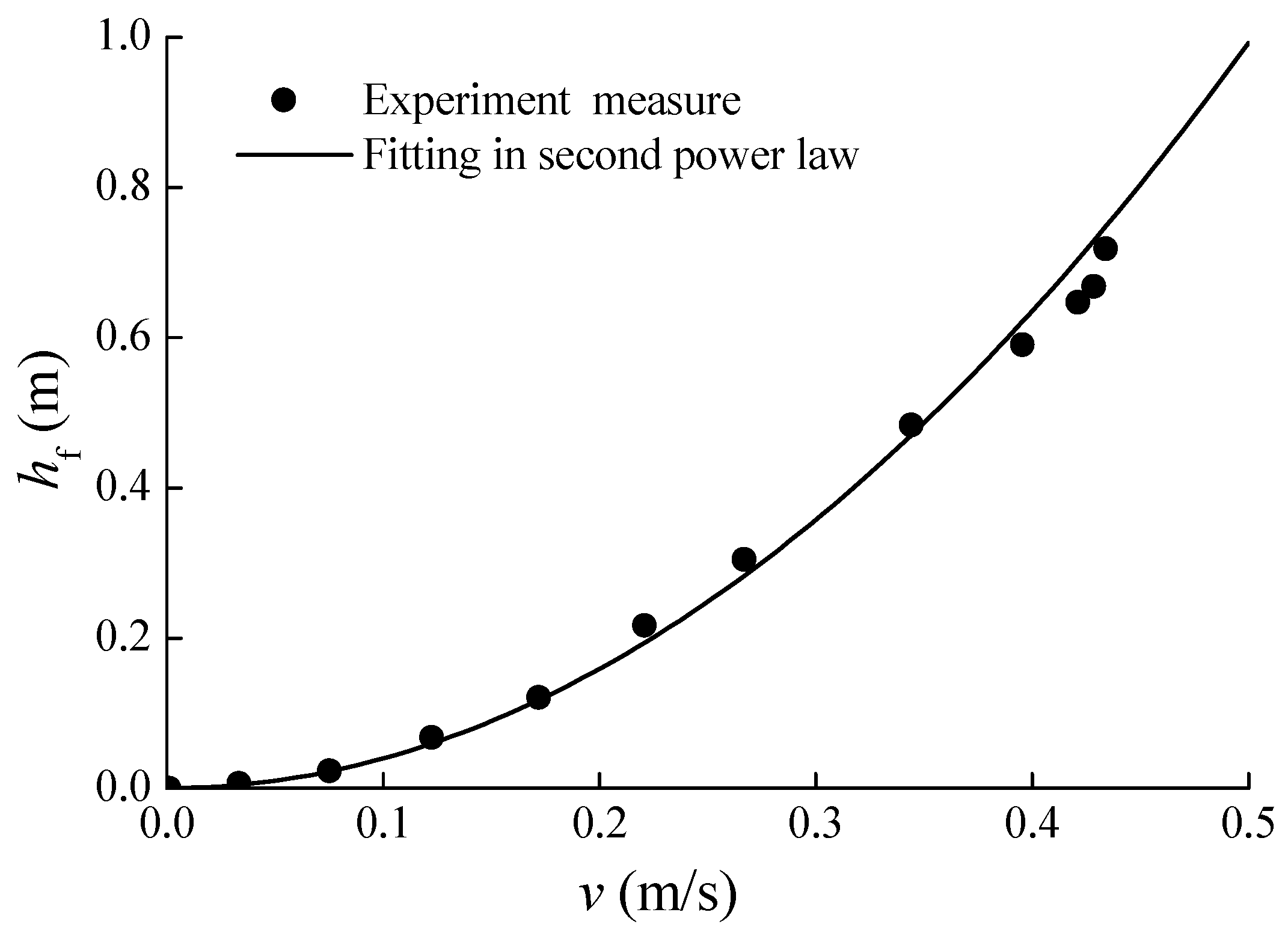
The hydraulic head loss is an important factor for water hammer. Traditional water hammer simulations commonly approximate friction resistance based on the steady status. In order to consider total head loss, including minor loss, various velocity experiments are conducted. Various steady flow conditions of different flow velocities are accessed by controlling the upstream reservoir water level.
Two pressure sensors are set at the upstream side and downstream side of the pipeline respectively. The pressure difference of those two sensors represents the total head loss under the corresponding flow velocity. Figure 4 shows the total head loss change with the velocities, and the fitting friction curve is provided with an equivalent friction factor 0.269. It shows that the steady friction can be obtained by the second power law.
3.2. Valve Performance
Discharge properties of the valve can greatly affect the water hammer process. A relatively smooth valve-closing process can effectively reduce the water hammer strength. To numerically simulate the experimental transient process, it is always necessary preparatory work to measure the valve’s real discharge coefficient curve. To obtain the characteristics of the valve, the experimental data of various steady flow conditions are recorded. Adjusting the open ratio of the valve, according to the corresponding water head difference at two sides and the flow discharge through the valve, several mapping relationship dots are recorded based on Equation (15). After a least square method fitting, the performance curve of the valve in the experiment is shown in Figure 5.
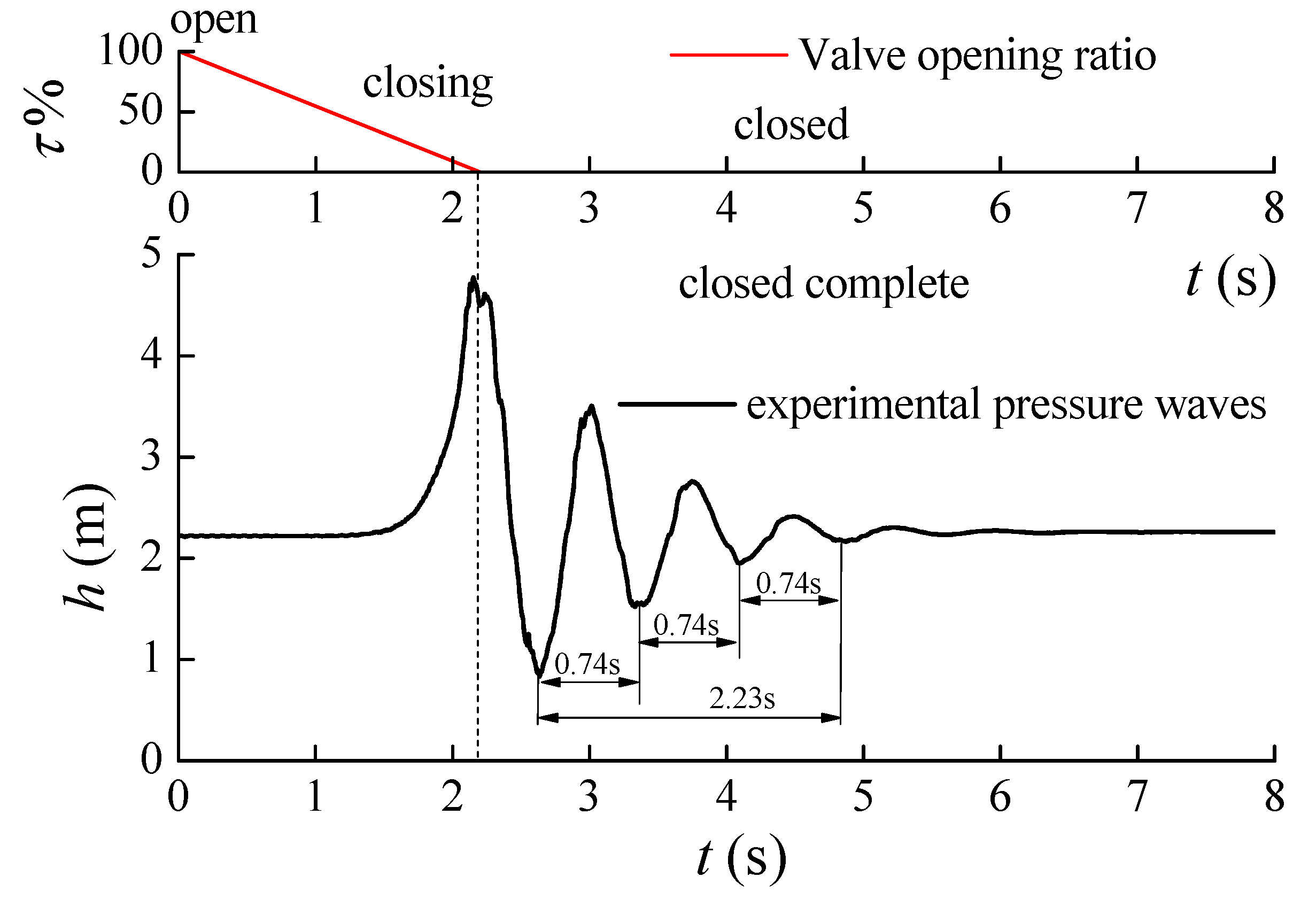
3.3. Water Hammer Measurements
A related experiment was conducted in order to validate and improve the model. As shown in Figure 2, the experiment consists of a straight pipe, valves, and upstream reservoir. In the system, the length of the pipe is 29 m and the internal diameter is 0.107 m. A water hammer is generated when the valve is closed in 2.2 s. Figure 6 shows the water hammer pressure process. As seen in the figure, the wave-shaped curve shows the stable frequency and periods.
According to the periods and length of the travel path, the experimental wave speed can be determined as follows
The experimental wave speed is only about 151.0 m/s. However, without taking into account the air, the intrinsic wave speed in the pipe should be about 1340 m/s according to the water hammer wave speed formula. Obviously, the experimental wave speed is far lower than for a pipe without air, because of air entrainment. For pipe flow with air content [1], the relationship between air content and the shock wave speed is
where is the actual wave velocity in a pipe system, is the volume modulus, is the density, is the elasticity modulus, and is the amount of substance of the gas in unit volume. Provided with the actual experimental wave speed, the air content can be evaluated as
For the case shown in Figure 6, the amount of air per unit volume is about 0.205, and air volume content is about 0.459% according to this measurement.
Thus, all the necessary coefficients are established, which provide the basic parameters required to numerically simulate the water hammer process.
4. Simulation and Analysis
4.1. Simulation and Comparison
Above we presented the LWM model for general internal nodes, and a matching boundary conditions model was also established. In order to debug the proposed model, the pipe system in Figure 2 is simulated and compared with MOC. The performance of the valve is shown in Figure 5. Figure 7 shows the numerical solution of the water hammer process produced in the condition that the valve is closed in 2.2 s. As shown in the figure, the proposed model is in agreement with the MOC; indeed, they can almost produce the same numerical simulation. However, a small difference can be found in the phase of the wave. Obviously, the phase difference increases with time, because the proposed model considers the influence of the pipe flow velocity on the wave propagation. With a lower speed, the flow speed can be considered by the convective term. As shown in Figure 7, both LWM and MOC can give out reasonable maximum pressure, which is the key to water hammer prediction.
4.2. Improvement to Approximate the Attenuation
As seen in Figure 7, the LWM can simulate the actual maximum water hammer pressure. It may meet the common requirement for predicting and preventing water hammer overpressure. However, the numerical results heavily distorted the properties of the attenuation, compared to the experimental result. After the complete closing of the valve, the peak pressure of the water hammer wave decreases rapidly in the experiment, but the water hammer wave decreases slowly in the numerical simulation. Obviously, the attenuation is heavily underestimated in the numerical simulation. In order to modify the deviation, an additional friction function is introduced according to the flow patterns.
In Figure 7, the numerical model evaluates the unsteady friction resistance according to the experimental measurement shown in Figure 4, which denotes the steady friction in pipe flow. The model can simulate a water hammer well before the valve has closed completely, and during this period the pipe flow maintained positive velocity. However, after the valve is completely closed, the fluid will have a great impact on the pipeline, and then the steady friction cannot actually approximate the practical energy dissipation. The experiment can actually measure the attenuation process of the water hammer wave, but it cannot measure the impact flow rate and the actual energy dissipation. In order to evaluate the attenuation, an additional friction function is introduced to the numerical model. The friction term is proposed as follows
where is the proposed additional function after the valve’s complete closing, which can be described as . where is the valve closing time.
Considering a, m, g and L as the main physical variables, combining the Darcy-Weisbach friction factor, the additional function can be described as
where is the Darcy-Weisbach friction factor. According to Rayleigh’s method of dimensional analysis, the exponential function is proposed as
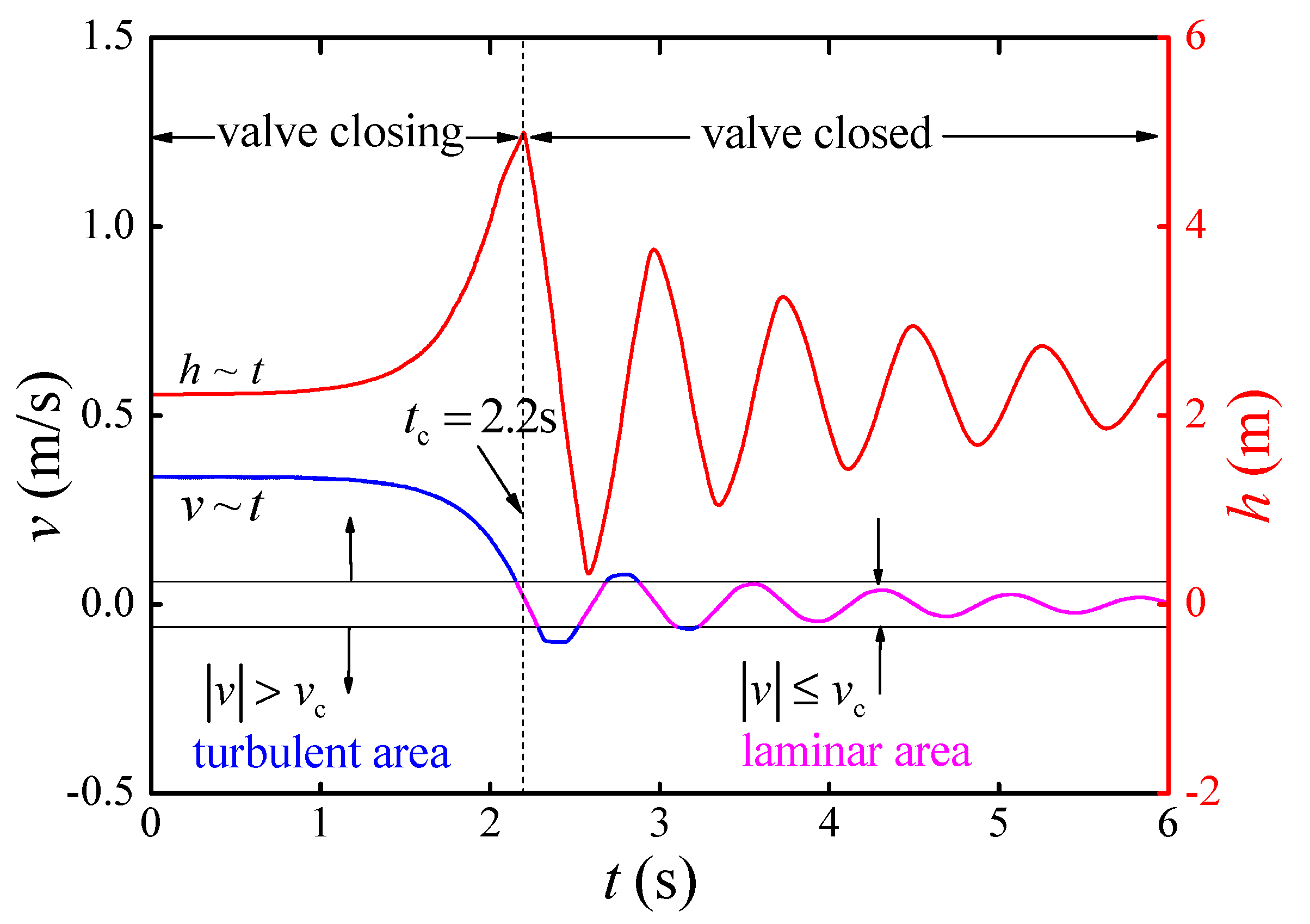
where C is a dimensionless coefficient that needs to be calibrated by experiment. After a complete valve closing, the flow is only impacted at low velocity. According to the flow patterns, the can separately be described as in laminar model (LM) and in turbulent model (TM) [35]. Figure 8 shows that the flow velocity may cross laminar and turbulent zones during hydraulic transient. The compound model (CM) can be described as
where is the critical flow velocity between laminar and turbulent flow.
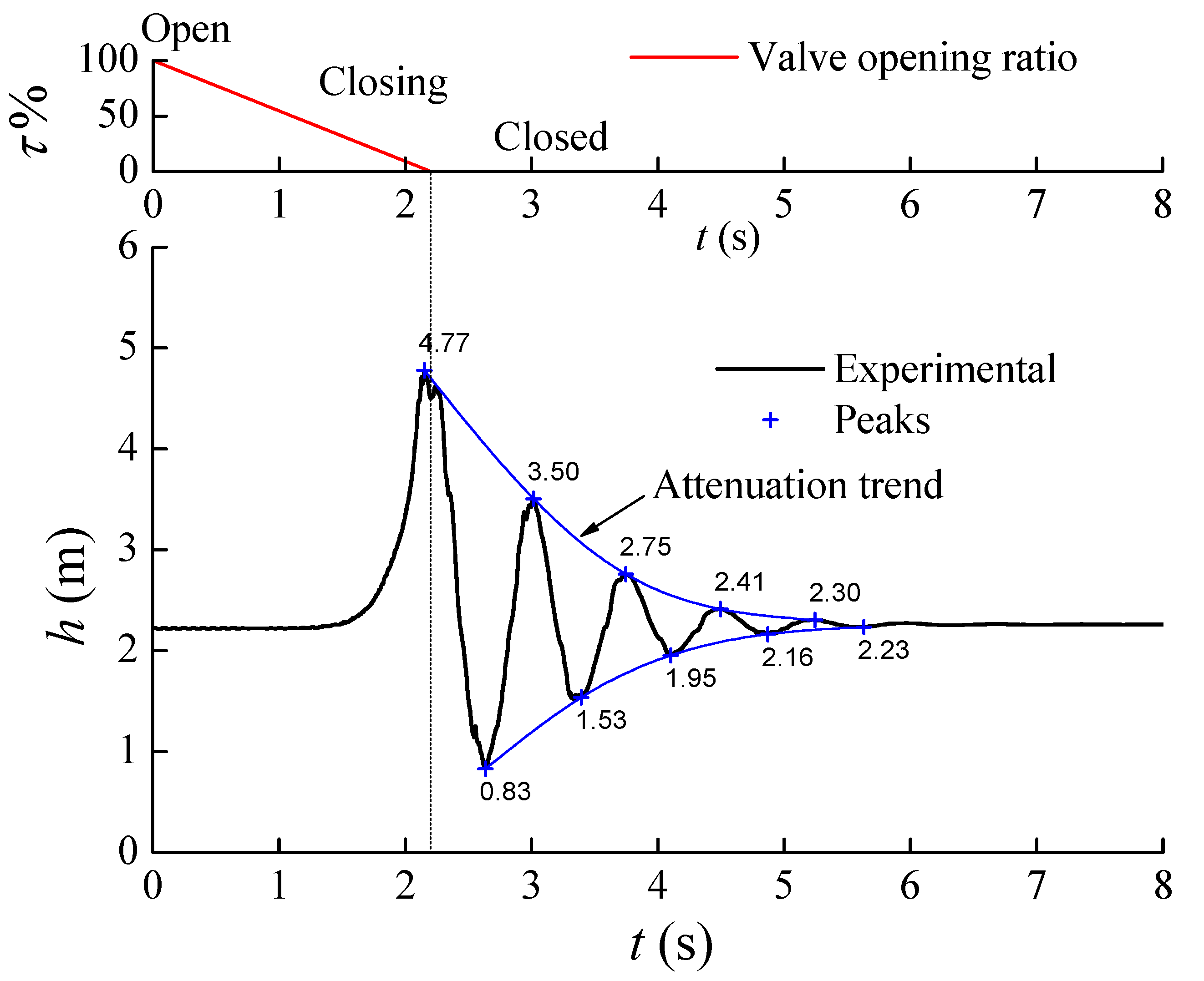
In order to calibrate the dimensionless coefficient C, the positive and negative peaks are identified and analyzed in Figure 9.
Based on the identified peaks, the method of least squares is used to obtain the optimal C. The squared residuals between experimental and simulated peaks are defined as
Then, the sum of squared residuals is
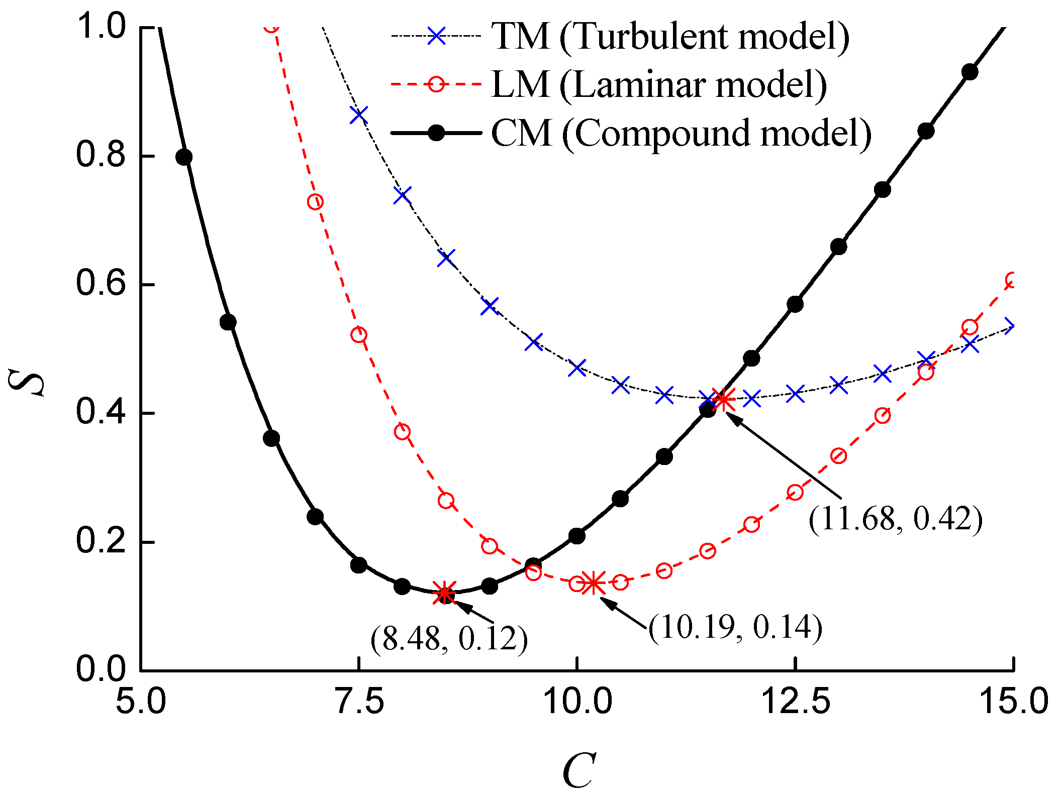
The optimal C can be determined when the sum of squared residuals is the least. In order to optimize the dimensionless coefficient C, the water hammer processes are simulated by various dimensionless coefficients and three kinds of friction models. The relationship between the sum of squared residuals and the dimensionless coefficient C in each model are shown in Figure 10. Table 1 shows the first 10th peaks of the optimized simulations in each model. The result shows that the CM model can give the least sum of squared residuals, in which the matched coefficient is about 8.48. Then the additional function is written as
Figure 11 compares the water hammer simulations. Obviously, the improved model can more actually simulate the attenuation.
By introducing the additional friction function, the improved model can simulate water hammer more actually, not only on the maximum pressure, but also the attenuation of the water hammer waves.
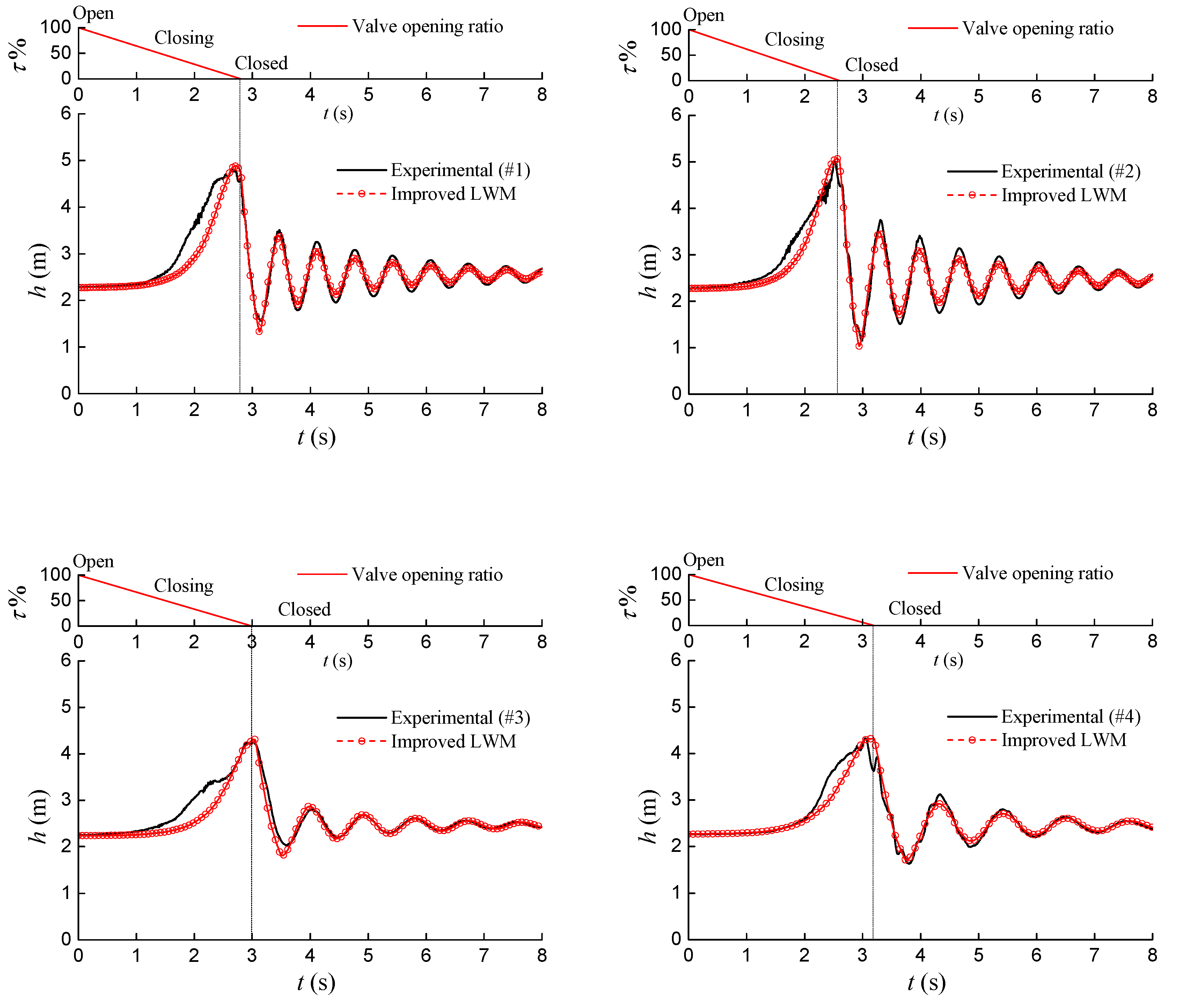
For validation, the improved model is applied to various air-water mixtures conditions as shown in Table 2. Changing the valve closing time and the air mass entrainment, various water hammer processes are produced. These water hammers are experimentally measured and numerically simulated. Although the actual air content is hard to measure, it can be estimated by the actual wave speed according to previous research [1]. In the numerical model, the air content is taken into account by adjusting in Equation (26), the amount of substance of the gas in unit volume, which affects the energy loss degree greatly. This is inferred from the measured actual wave speed in experiment using Equation (19). As shown in Figure 12, the numerical simulation results using the improved LWM are in agreement with the experimental results both on the maximum pressure and the attenuation trends.
5. Discussion
The LWM is widely used in computational fluid dynamics for fluid field simulation. However, it is uncommonly used in numerical water hammer-simulation for pipe systems. As an alternative approach, LWM can be applied to the water hammer hyperbolic partial differential equations system. In particular, the convective acceleration terms are completely considered in the model, although they only affect the water hammer slightly. Considering the applicability in numerical computation, the LWM can yield the water hammer maximum pressure as the MOC, which shows that the LWM can suit the water hammer equations. However, considering the water hammer experiment in the pipe, LWM may heavily distort the attenuation of the water hammer wave. Based on the experiment, an additional friction function is proposed to simulate the actual wave attenuation. Traditional numerical simulations greatly underestimate air resistance when the valve is closed completely. By introducing the additional resistance function, the proposed model can simulate the water hammer well, both on the maximum pressure and the attenuation process. In particular, it is difficult to reveal the mechanism of the resistance in the shock flow after completely closing valve. Many studies have reported the difference of the water hammer attenuation process in theory and experiment. Traditional models underestimate the resistance, which makes the fluctuation remain longer in the numerical result. Considering the restriction of the experimental scale of the pipe used in this research on the water hammer in gravitational pipe flow system with air entrainment, it may require a different friction coefficient in flow with air content after complete valve closing.
6. Conclusions
Based on the Lax-Wendroff difference Method, a numerical water hammer model is established for gravitational flow pipe systems. The proposed model considers the influence of convective acceleration terms, and it also supports flexibly setting the time steps and space steps without the limitation of the characteristics in MOC. With a second-order accuracy, the model is validated by MOC and used in an experiment to predict the maximum transient pressures. The experiment shows that the water hammer processes in water supply systems with air entrainment differ much from those in one phase of pure water, especially on the attenuation processes. The improved model with a modified friction function using a compound model can simulate the water hammer processes well, both on the maximum pressures and the attenuation process. This research reveals that we used to underestimate the energy loss process of a water hammer in pipe systems, especially in conditions with air content. Proposed improved LWM can simulate water hammers much better in such conditions. As plenty of practical water supply systems are running with air content, this research can be helpful on predicting water hammers in actual engineering.
In further research, the physical interaction of air entrainment in water hammer processes and the air-delivery process in a water hammer will be researched. To figure out the air inlet conditions and its physical interactions, a further experiment will be conducted using a tube with a visible interior to observe the air-delivery trail and its shape-changing process in water hammers.
Author Contributions
Methodology, B.Z.; Validation, B.Z.; Investigation, B.Z.; Experiment, B.Z., M.S.; Data-curation, M.S.; Original writing, B.Z.; Resources, W.W.; Visualization, W.W.; Supervision, W.W.; Project administration, W.W.; Funding acquisition W.W.
Funding
This research work was funded by the National Natural Science Foundation of China (Grant Nos. 51779216, 51279175) and Zhejiang Provincial Natural Science Foundation of China (Grant No. LZ16E090001).
Conflicts of Interest
The authors declare no conflicts of interest.
Nomenclature
| = | acceleration of gravity (m/s2) | |
| = | pressure head (m) | |
| = | distance along pipe from inlet (m) | |
| = | time, as subscript to denote time (s) | |
| = | flow velocity (m/s) | |
| = | Darcy friction factor | |
| = | main pipe diameter (m) | |
| = | the angle between pipe and the horizontal plane. | |
| = | speed of pressure wave (m/s) | |
| = | serial number of nodes (s) | |
| = | time step (s) | |
| = | number of sections | |
| = | length of segment (m) | |
| = | head of upstream reservoir (m) | |
| = | discharge coefficient | |
| = | the height of reference plane | |
| = | head drop due to friction along the pipe (m) | |
| = | valve opening ratio | |
| = | volume modulus | |
| = | density (kg/m3) | |
| = | elasticity modulus of steel pipe | |
| = | thickness of steel pipe (m) | |
| = | air content occupied in mixed fluid | |
| = | thermodynamics constant (J/(mol∙K)) | |
| = | temperature (K) | |
| = | absolute pressure (pa) | |
| = | additional friction factor in two-phase flow | |
| = | length of the pipe (m) | |
| = | additional friction factor after valve closed completely | |
| = | time of valve closing operation | |
| = | coefficient in additional friction function | |
| = | kinematic viscosity of water (m2/s) | |
| = | hydraulic radius (m) | |
| = | the critical flow velocity between laminar and turbulent flow (m/s) | |
| = | residuals between experimental and simulated peaks (m) | |
| = | the sum of squared residuals | |
| = | experimental positive peak (m) | |
| = | experimental negative peak (m) | |
| = | experimental positive peak (m) | |
| = | experimental negative peak (m) |
Acronyms
| MOC | = | Method of Characteristics |
| LWM | = | Lax-Wendroff Method |
References
- Wylie, E.B.; Streeter, V.L.; Suo, L. Fluid Transients in Systems; Prentice Hall: Englewood Cliffs, NJ, USA, 1993. [Google Scholar]
- Yu, X.D.; Zhang, J.; Miao, D. Innovative Closure Law for Pump-Turbines and Field Test Verification. J. Hydraul. Eng. 2015, 141, 9. [Google Scholar] [CrossRef]
- Chaudhry, M. Applied Hydraulic Transients; Van Nostrana Reinhold Co.: New York, NY, USA, 1987. [Google Scholar]
- Besharat, M.; Viseu, M.T.; Ramos, H.M. Experimental Study of Air Vessel Behavior for Energy Storage or System Protection in Water Hammer Events. Water 2017, 9, 63. [Google Scholar] [CrossRef]
- Coronado-Hernandez, O.E.; Fuertes-Miquel, V.S.; Besharat, M.; Ramos, H.M. Experimental and Numerical Analysis of a Water Emptying Pipeline Using Different Air Valves. Water 2017, 9, 98. [Google Scholar] [CrossRef]
- Wood, D.J. Waterhammer analysis-Essential and easy (and efficient). J. Environ. Eng.-Asce 2005, 131, 1123–1131. [Google Scholar] [CrossRef]
- Tijsseling, A.S.; Anderson, A. Thomas Young’s research on fluid transients: 200 years on. In Proceedings of the 10th International Conference on Pressure Surges, Edinburgh, UK, 14–16 May 2008; Hunt, S., Ed.; BHR Group Limited: Cranfield, UK, 2008. [Google Scholar]
- Tijsseling, A.S.; Anderson, A. A Precursor in Waterhammer Analysis-Rediscovering Johannes von Kries. In Proceedings of the 9th International Conference on Pressure Surges, Chester, UK, 24–26 March 2004; Murray, S.J., Ed.; BHR Group Limited: Cranfield, Bedfordshire, UK, 2004. [Google Scholar]
- Ghidaoui, M.S.; Zhao, M.; McInnis, D.A.; Axworthy, D.H. A review of water hammer theory and practice. Appl. Mech. Rev. 2005, 58, 49–76. [Google Scholar] [CrossRef]
- Triki, A. Dual-technique-based inline design strategy for water hammer control in pressurized pipe flow. Acta Mech. 2018, 229, 2019–2039. [Google Scholar] [CrossRef]
- Zhang, X.X.; Cheng, Y.G.; Xia, L.S.; Yang, J.D. CFD simulation of reverse water hammer induced by collapse of draft-tube cavity in a model pump-turbine during runaway process. In Proceedings of the 28th Iahr Symposium on Hydraulic Machinery and Systems, Grenoble, France, 4–8 July 2016. [Google Scholar]
- Chaudhry, M.; Hussaini, M. Second-order accurate explicit finite-difference schemes for waterhammer analysis. J. Fluids Eng. 1985, 107, 523–529. [Google Scholar] [CrossRef]
- Kochupillai, J.; Ganesan, N.; Padmanabhan, C. A new finite element formulation based on the velocity of flow for water hammer problems. Int. J. Press. Ves. Pip. 2005, 82, 1–14. [Google Scholar] [CrossRef]
- Tian, W.X.; Su, G.H.; Wang, G.P.; Qiu, S.Z.; Xia, Z.J. Numerical simulation and optimization on valve-induced water hammer characteristics for parallel pump feedwater system. Ann. Nuclear Energy 2008, 35, 2280–2287. [Google Scholar] [CrossRef]
- Schmitt, C.; Pluvinage, G.; HADJ-TAIEB, E.; Akid, R. Water pipeline failure due to water hammer effects. Fatigue Fract. Eng. Mater. Struct. 2006, 29, 1075–1082. [Google Scholar] [CrossRef]
- Karadžić, U.; Bulatović, V.; Bergant, A. Valve-Induced Water Hammer and Column Separation in a Pipeline Apparatus. Stroj. Vestn.-J. Mech. Eng. 2014, 60, 742–754. [Google Scholar]
- Izquierdo, J.; Iglesias, P.L. Mathematical modelling of hydraulic transients in simple systems. Math. Comput. Modell. 2002, 35, 801–812. [Google Scholar] [CrossRef]
- Bazargan-Lari, M.R.; Kerachian, R.; Afshar, H.; Bashi-Azghadi, S.N. Developing an optimal valve closing rule curve for real-time pressure control in pipes. J. Mech. Sci. Technol. 2013, 27, 215–225. [Google Scholar] [CrossRef]
- Wan, W.; Li, F. Sensitivity Analysis of Operational Time Differences for a Pump-Valve System on a Water Hammer Response. J. Press. Vess. Technol. 2016, 138, 011303. [Google Scholar] [CrossRef]
- Sibetheros, I.A.; Holley, E.R.; Branski, J.M. Spline Interpolations for Water Hammer Analysis. J. Hydraul. Eng.-ASCE 1991, 117, 1332–1351. [Google Scholar] [CrossRef]
- Gong, J.Z.; Lambert, M.F.; Simpson, A.R.; Zecchin, A.C. Detection of Localized Deterioration Distributed along Single Pipelines by Reconstructive MOC Analysis. J. Hydraul. Eng. 2014, 140, 190–198. [Google Scholar] [CrossRef] [Green Version]
- Travas, V.; Basara, S. A mixed MOC/FDM numerical formulation for hydraulic transients. Tehn. Vjesn.-Techn. Gazette 2015, 22, 1141–1147. [Google Scholar]
- Evangelista, S.; Leopardi, A.; Pignatelli, R.; de Marinis, G. Hydraulic Transients in Viscoelastic Branched Pipelines. J. Hydraul. Eng. 2015, 141, 04015016. [Google Scholar] [CrossRef]
- Covas, D.; Stoianov, I.; Mano, J.F.; Ramos, H.; Graham, N.; Maksimovic, C. The dynamic effect of pipe-wall viscoelasticity in hydraulic transients. Part I-experimental analysis and creep characterization. J. Hydraul. Res. 2004, 42, 516–530. [Google Scholar] [CrossRef]
- Wood, D.J.; Lingireddy, S.; Boulos, P.F.; Karney, B.W.; McPherson, D.L. Numerical methods for modeling transient flow in distribution systems. J. Am. Water Work Assoc. 2005, 97, 104–115. [Google Scholar] [CrossRef]
- Guo, L.L.; Geng, J.; Shi, S.; Du, G.S. Study of the Phenomenon of Water Hammer Based on Sliding Mesh Method. In Development of Industrial Manufacturing; Choi, S.B., Hamid, F.S., Han, L., Eds.; Scientific.net: Zurich, Switzerland, 2014; Volume 525, pp. 236–239. [Google Scholar]
- Hwang, Y.H. Development of a particle method of characteristics (PMOC) for one-dimensional shock waves. Shock Waves 2018, 28, 379–399. [Google Scholar] [CrossRef]
- Zhou, L.; Wang, H.; Liu, D.Y.; Ma, J.J.; Wang, P.; Xia, L. A second-order Finite Volume Method for pipe flow with water column separation. J. Hydrol.-Environ. Res. 2017, 17, 47–55. [Google Scholar] [CrossRef]
- Bergant, A.; Tusseling, A.S.; Vitkovsky, J.P.; Covas, D.I.C.; Simpson, A.R.; Lambert, M.F. Parameters affecting water hammer wave attenuation, shape and timing—Part 1: Mathematical tools. J. Hydraul. Res. 2008, 46, 373–381. [Google Scholar] [CrossRef]
- Bergant, A.; Tijsseling, A.S.; Vitkovsy, J.P.; Covas, D.I.C.; Simpson, A.R.; Lambert, M.F. Parameters affecting water hammer wave attenuation, shape and timing-Part 2: Case studies. J. Hydraul. Res. 2008, 46, 382–391. [Google Scholar] [CrossRef]
- Zhou, F.; Hicks, F.E.; Asce, M.; Steffler, P.M. Transient flow in a rapidly filling horizontal pipe containing trapped air. J. Hydraul. Eng.-ASCE 2002, 128, 625–634. [Google Scholar] [CrossRef]
- Anderson, J.D. Computational Fluid Dynamics: The Basics with Applications; McGrawhill Inc.: New York, NY, USA, 1995. [Google Scholar]
- Manopoulos, C.G.; Mathioulakis, D.S.; Tsangaris, S.G. One-dimensional model of valveless pumping in a closed loop and a numerical solution. Phys. Fluids 2006, 18, 017106. [Google Scholar] [CrossRef]
- Himr, D. Numerical simulation of water hammer in low pressurized pipe: comparison of SimHydraulics and Lax-Wendroff method with experiment. In Proceedings of the EPJ Web of Conferences, Hradec Králové, Czech Republic, 20–23 November 2012; Dancova, P., Novonty, P., Eds.; Technical University of Liberec: Liberec, Czech Republic, 2012. [Google Scholar]
- Wan, W.Y.; Zhu, S.; Hu, Y.J. Attenuation analysis of hydraulic transients with laminar-turbulent flow alternations. Appl. Math. Mech. 2010, 31, 1209–1216. [Google Scholar] [CrossRef]
Figure 1.
Meshes and node types.
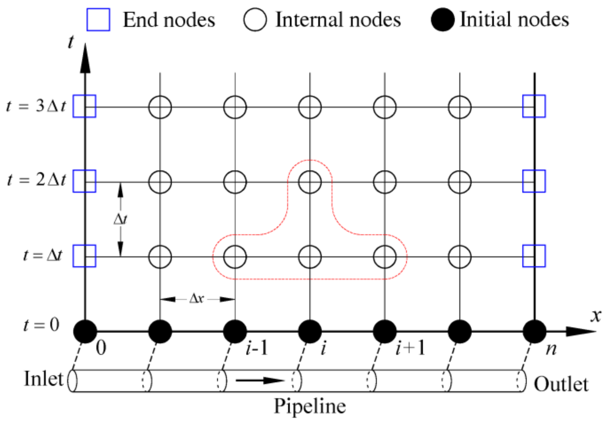
Figure 2.
Pipe flow system for water hammer analysis.
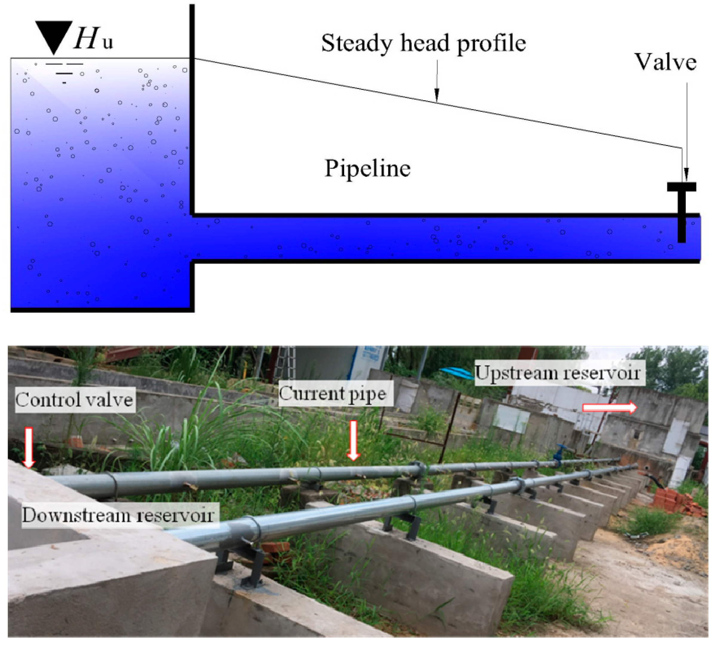
Figure 3.
Boundary model of the pipe ends.
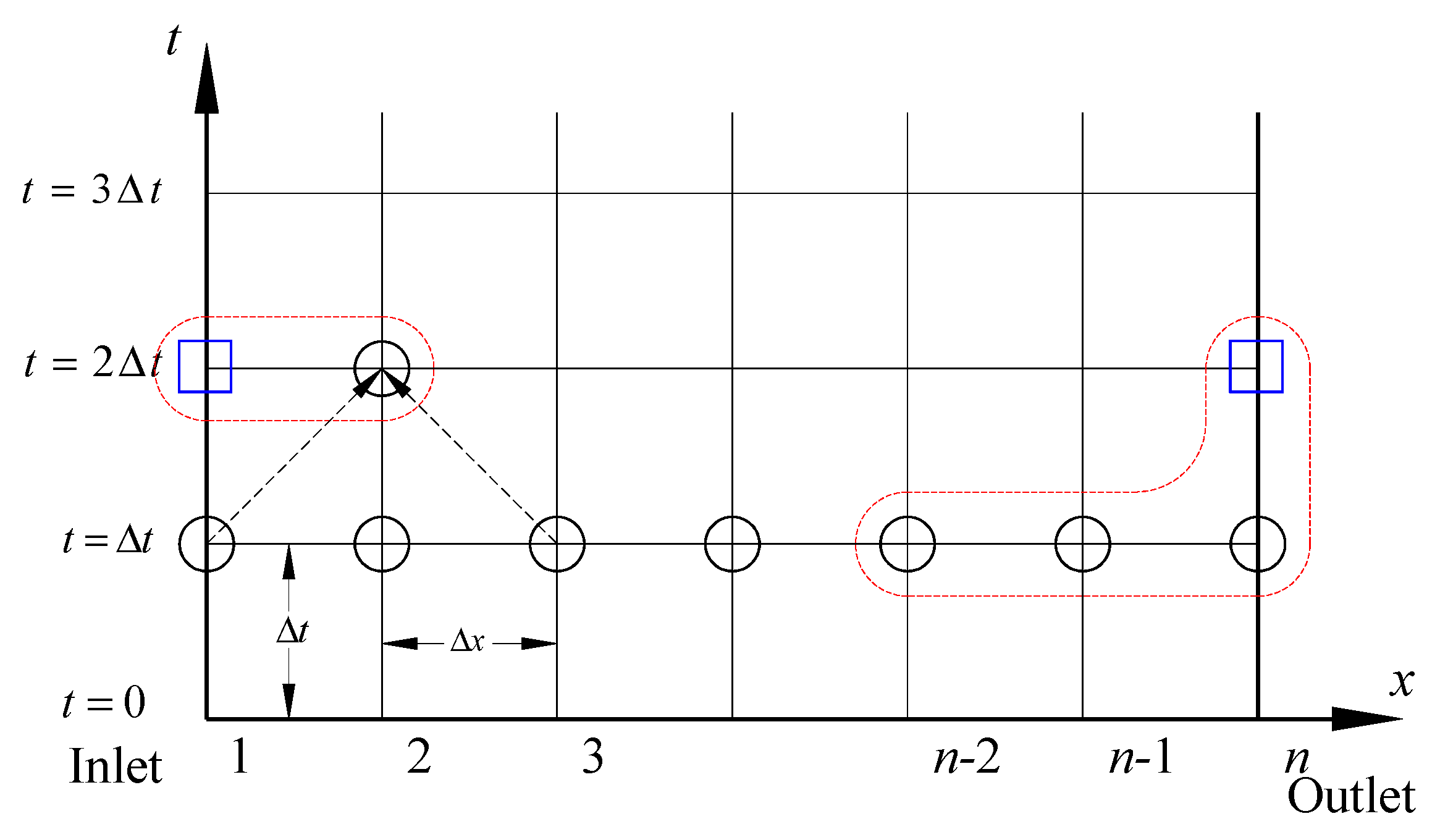
Figure 4.
Measurement of hydraulic head loss in steady flow.

Figure 5.
The experimental discharge coefficient of the valve.
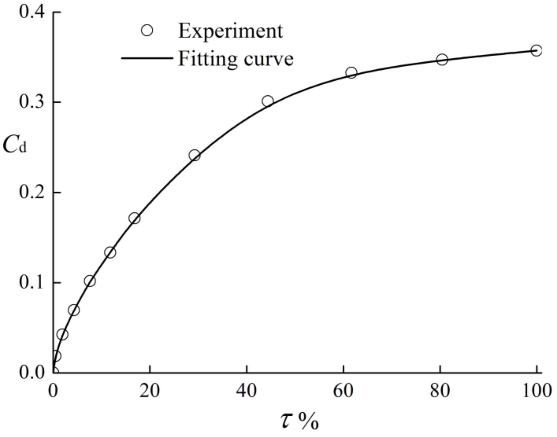
Figure 6.
Experimental water hammer progress.

Figure 7.
The transient-pressure process.
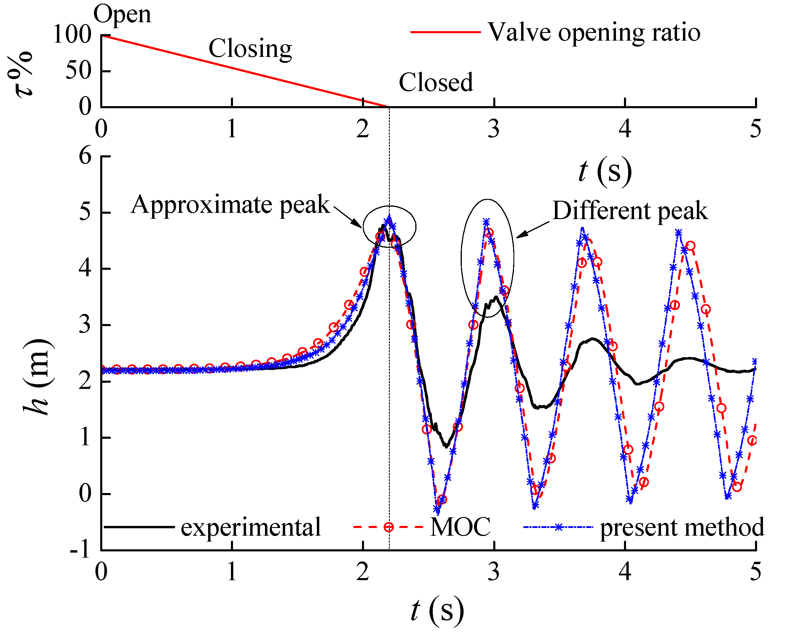
Figure 8.
The flow velocity process during hydraulic transient.

Figure 9.
The positive and negative peaks in experimental measurement.

Figure 10.
The analysis of the sum of squared residuals.

Figure 11.
Simulation by improved two-phase model.
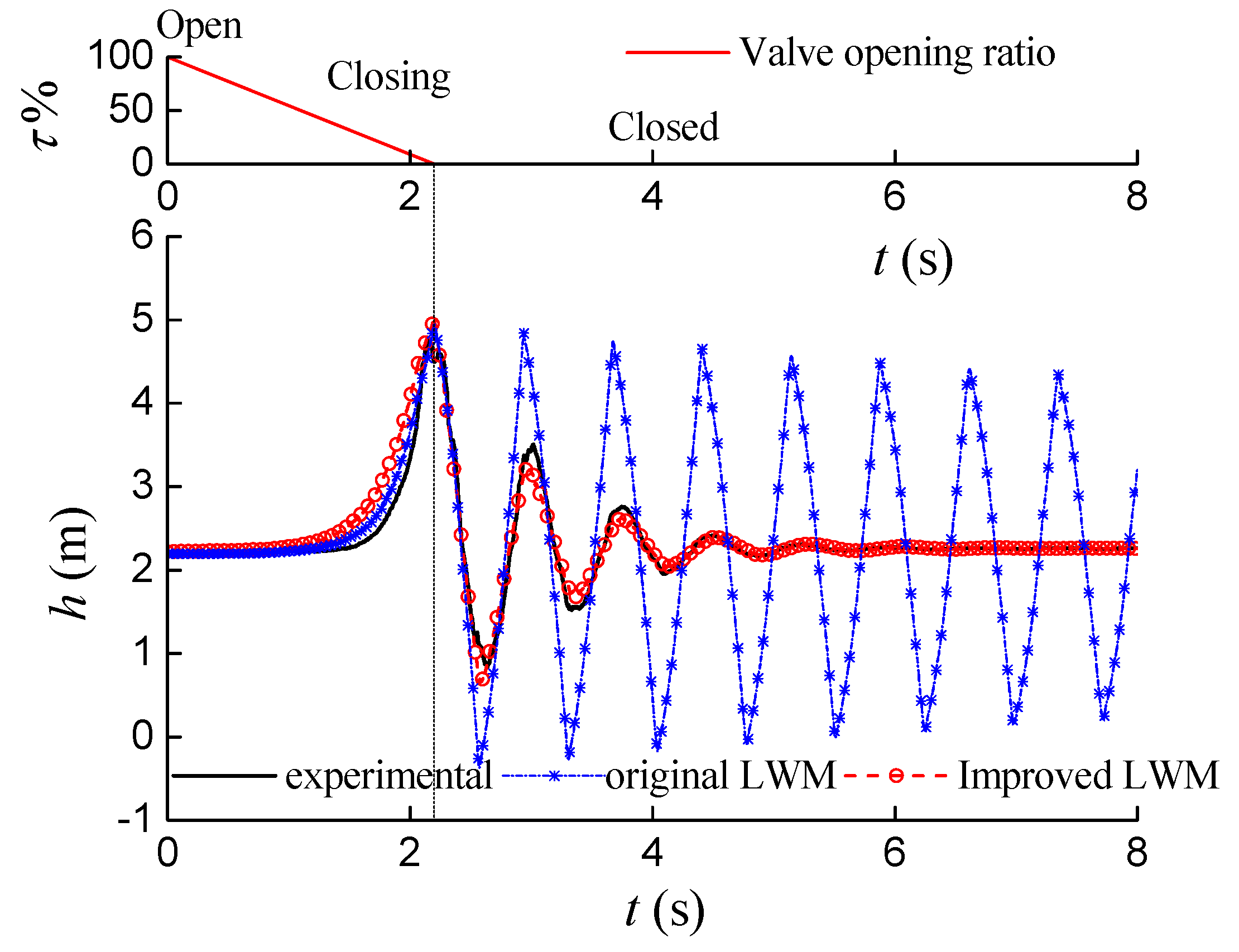
Figure 12.
Application of the improved model to water hammer simulations.

Table 1.
The attenuation of peak pressures from experiment and improved simulations.
| Periods | Experimental | Original | Improved | |||||||
|---|---|---|---|---|---|---|---|---|---|---|
| LM | TM | CM | ||||||||
| 1st | 4.77 | 0.83 | 4.96 | −0.38 | 4.93 | 0.66 | 4.94 | 1.01 | 4.93 | 0.66 |
| 2nd | 3.50 | 1.53 | 4.84 | −0.27 | 3.22 | 1.68 | 3.08 | 1.65 | 3.23 | 1.68 |
| 3rd | 2.75 | 1.95 | 4.74 | −0.17 | 2.61 | 2.04 | 2.74 | 1.86 | 2.62 | 2.04 |
| 4th | 2.41 | 2.16 | 4.65 | −0.09 | 2.39 | 2.18 | 2.60 | 1.96 | 2.39 | 2.18 |
| 5th | 2.30 | 2.23 | 4.56 | 0.00 | 2.31 | 2.23 | 2.52 | 2.02 | 2.31 | 2.23 |
Table 2.
Various valve closing speed simulations for validation.
| Case | Wave Speed (m∙s−1) | m | Air Content (%) | Closing Time (s) |
|---|---|---|---|---|
| #1 | 183 | 0.139 | 0.308 | 2.8 |
| #2 | 175 | 0.152 | 0.338 | 2.6 |
| #3 | 132 | 0.269 | 0.598 | 3.0 |
| #4 | 110 | 0.388 | 0.864 | 3.2 |
© 2018 by the authors. Licensee MDPI, Basel, Switzerland. This article is an open access article distributed under the terms and conditions of the Creative Commons Attribution (CC BY) license (http://creativecommons.org/licenses/by/4.0/).
Share and Cite
MDPI and ACS Style
Zhang, B.; Wan, W.; Shi, M. Experimental and Numerical Simulation of Water Hammer in Gravitational Pipe Flow with Continuous Air Entrainment. Water 2018, 10, 928. https://doi.org/10.3390/w10070928
AMA Style
Zhang B, Wan W, Shi M. Experimental and Numerical Simulation of Water Hammer in Gravitational Pipe Flow with Continuous Air Entrainment. Water. 2018; 10(7):928. https://doi.org/10.3390/w10070928
Chicago/Turabian StyleZhang, Boran, Wuyi Wan, and Mengshan Shi. 2018. "Experimental and Numerical Simulation of Water Hammer in Gravitational Pipe Flow with Continuous Air Entrainment" Water 10, no. 7: 928. https://doi.org/10.3390/w10070928
Note that from the first issue of 2016, this journal uses article numbers instead of page numbers. See further details here.