Article

Interaction between Perched Epikarst Aquifer and Unsaturated Soil Cover in the Initiation of Shallow Landslides in Pyroclastic Soils

by
Roberto Greco
*,
Pasquale Marino
,
Giovanni Francesco Santonastaso
and
Emilia Damiano
Dipartimento di Ingegneria, Università degli Studi della Campania ‘L. Vanvitelli’, via Roma 9, 81031 Aversa (CE), Italy
*
Author to whom correspondence should be addressed.
Water 2018, 10(7), 948; https://doi.org/10.3390/w10070948
Submission received: 28 June 2018 / Revised: 10 July 2018 / Accepted: 13 July 2018 / Published: 16 July 2018
(This article belongs to the Special Issue Landslide Hydrology)

Abstract

:
A physically based mathematical model of the slope of Cervinara (southern Italy), which is characterized by a shallow pyroclastic soil cover laying upon a limestone fractured bedrock, has been developed. Previous and current ongoing monitoring suggested that leakage through the soil–bedrock interface occurred, with leaking water temporarily stored in a perched aquifer located in the upper part of the fractured limestone (epikarst). This aquifer supplied several springs, and recharge to the deeper groundwater circulation occurred. Hence, in the proposed model, the unsaturated water flow taking place within the soil cover is coupled with the saturated water flow in the perched aquifer. The application of the model to the simulation of the slope hydrologic behavior over a period of 11 years, between 2006–2017, provides realistic results in terms of soil storage, epikarst storage, spring discharge, and groundwater recharge. The different response times of soil and epikarst aquifer to precipitation input allow distinguishing the hydrological predisposing causes of potential landsliding (i.e., a few months of persistent rainfall that is capable of filling the epikarst aquifer) from the triggers, which are represented by single intense rainfall events. The application of the model offers a key of interpretation of the hydrological processes leading to the landslide that occurred on 16 December 1999.

1. Introduction

Rainfall-induced landslides in shallow granular soil covers are among the most hardly predictable landslide types. In fact, the initiation of such landslides strongly depends on the characteristics of the triggering rainfall event (e.g., duration, mean intensity, peak intensity), as well as on the moisture conditions of the potentially unstable soil layer at the onset of the event e.g., Crozier et al. [1,2,3,4]. The triggering of shallow landslides requires an increased storage of water within the soil cover, leading to pore pressure increase [5]. Hence, the correct assessment of the water balance of the soil cover is mandatory, considering infiltration as well as drainage mechanisms that are both strongly and non-linearly affected by the initial soil moisture state e.g., Tromp-van Meerveld et al., Nieber and Sidle, Damiano et al. [6,7,8]. Particularly, the hydraulic behavior of the boundaries of the soil cover, through which it exchanges water with the surrounding hydrological systems, needs to be understood [5]. In fact, it has also often been recognized in shallow soil covers that soil moisture follows a long-term trend e.g., Cascini et al., Comegna et al. [9,10], and so the initiation of landslides has been related by many authors to rainfall accumulated over various time intervals e.g., Glade et al., Chleborad et al. [11,12], which are in any case much longer than the triggering event duration. This confirms the role played by large-scale (in space and time) hydrological processes as the predisposing causes of landslides, with the triggering rainfall being only the last push for the slope to fail [13].
In Campania (southern Italy), steep slopes covered with a few meters of pyroclastic loose granular deposits, which are mainly ashes (sand to loamy sand) with some layers of pumices (sandy gravel) laying upon fractured limestone bedrock, are sometimes subjected to fast destructive flowslides e.g., Picarelli et al. [14]. Although it is commonly recognized that slope failure occurs when rainfall infiltration leads to the vanishing of the contribution to shear strength offered by soil suction in unsaturated conditions e.g., Lu and Likos, Greco and Gargano [15,16], the process leading to the establishment of such a condition is still debated. Many studies indicate that a prominent role is played by the hydraulic behavior of the soil–bedrock interface. In some cases, the interface is considered as poorly pervious, owing to the presence of a layer of fine-textured altered soil (silty sand) with low hydraulic conductivity [17,18]. In other studies, the interface is modeled as a capillary barrier due to the coarse dimension of limestone fractures, under the hypothesis that they contain air at atmospheric pressure [19]. Conversely, other authors consider the soil–bedrock interface pervious, and focus on the formation of perched aquifers within the fractured limestone, which affect the water potential of the unsaturated soil cover [20], and may give rise to exfiltration, thus favoring slope failure [21].
The fractured limestone rocks of Southern Apennines are indeed characterized by the presence of large karst aquifers, for which regional mean annual groundwater recharge up to 500 mm has been estimated, ranging between 30–200 mm in the part of Campania where the limestone is covered with pyroclastic deposits [22]. The exchange of water between the soil cover and the karst aquifer occurs through the epikarst, which is the upper part of the karst system, and is weathered and densely fractured, more permeable, and porous than the underlying carbonate rock [23]. Often, a perched aquifer develops in the epikarst, from which percolation through vertical fractures and the conduits ensure the recharge to the deep groundwater system [24,25]. The highly conductive and porous pyroclastic covers of Campania favor diffuse rainwater infiltration and the formation of a thick (up to 10–15 m) epikarst [26], storing water that is drained by temporary springs [27]. The fractures of the epikarst are usually filled with the overlying soil, are penetrated by tree roots, and contribute to evapotranspiration e.g., Bakalowicz, Jukic and Denic-Jukic [23,28], so that the hydraulic connection between the perched aquifer and the unsaturated soil cover is possible e.g., Fu et al. [29].
In this paper, based on the evidence from field monitoring carried out at the slope of Cervinara (about 40 km east of Naples), a simple physically based mathematical model is proposed that describes the interaction between the unsaturated pyroclastic soil cover and the underlying perched aquifer temporarily storing infiltrating water. Coupled modeling of unsaturated and saturated flows has been indeed shown to provide a better description of water exchanges between the vadose zone and shallow groundwater systems e.g., Xu et al., Szymkiewicz et al. [30,31] than traditional uncoupled approaches with static boundary conditions at the base of the unsaturated zone. The model is applied to the simulation of the hydrological response of the slope to precipitations for a 11-year period, showing how the water level in the perched aquifer may affect the water potential of the soil cover, allowing to reproduce the typical seasonal soil moisture variability observed in the field. Finally, the simulation of the response in 1999, when a catastrophic flowslide occurred on the night between 15–16 December, offers a possible key of interpretation of the process leading to the triggering of the landslide.

2. Materials and Methods

This study refers to the northeast slope of Mount Cornito, near the town of Cervinara, in Campania (southern Italy), which is located in the mountainous area about 40 km northeast of Naples (Figure 1). The slope was involved in a series of shallow landslides that occurred in an area of about 4 km2 during the night between 15–16 December 1999. The investigated area is part of the southern Apennines zone. The basal rock is Mesozoic–Cenozoic limestone, and the pyroclastic cover is mainly constituted by ashes (sand to loamy sand), with layers of pumiceous lapilli (sand with gravel). Near the interface with the bedrock, a layer of weathered ashes (silty sands) is present [18]. The slope ground surface has a regular inclination between 36° and 40° (Figure 1c). The deposit has the typical features found in the area, with the pumice layers only a few decimeters thick, while ashes reach a few meters. However, apart the foot of the slope, where accumulated colluvium reaches the depth of several meters of remolded material, the total thickness of the primary deposits rarely exceeds 2.5 m along the slope. Table 1 summarizes the main characteristics of the soils constituting the cover.
The climate is Mediterranean, with a mean annual precipitation of about 1600 mm, and total potential evapotranspiration, calculated with the empirical formula of Thornthwaite [32], between 700 mm (at the elevation of 750 m a.s.l.) and 800 mm (360 m a.s.l.). Table 2 reports the mean monthly values of potential evapotranspiration and precipitation measured between 2001–2017. The vegetation cover is mostly constituted by deciduous chestnut woods (Castanea sativa), which are cultivated for fruit production. In late spring and summer, a dense understory of brushes and ferns (Pteridium aquilinum) flourish. There are many perennial and intermittent springs all around the slopes of the area, which are mainly located near the foot of the slopes, but in some cases also along the slopes, at mid-altitude (Figure 2). The springs supply a network of small streams and creeks, all reaching the nearby river Isclero.

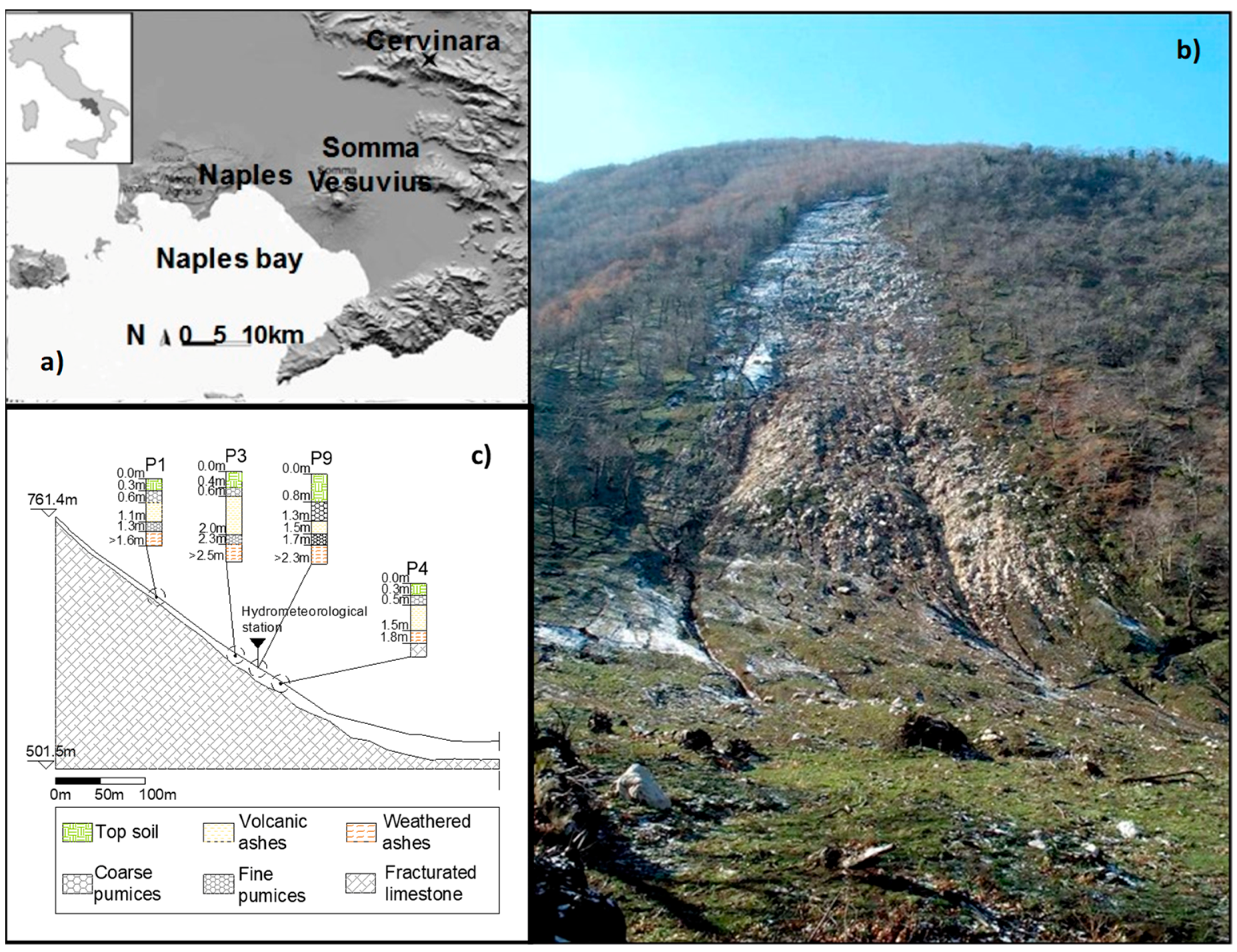
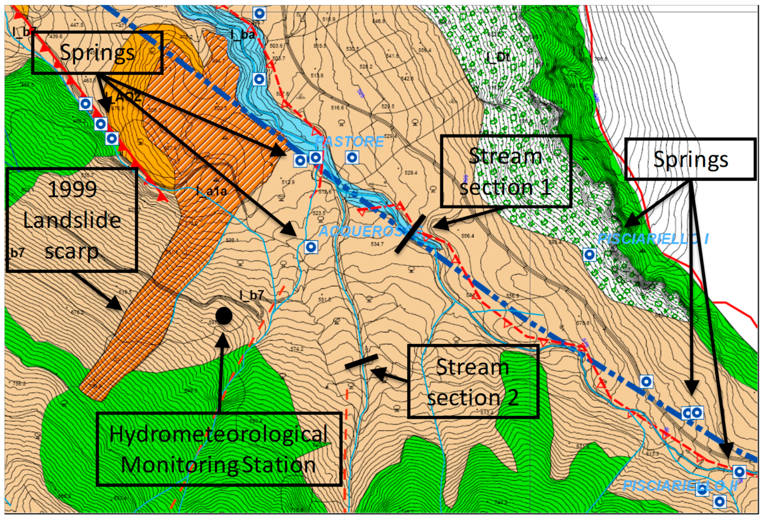
2.1. The Hydrometeorological Monitoring Station

Hydrological monitoring activities have been carried out at the slope of Cervinara since 2001. Initially, this was done by means of several tensiometers installed at various locations and depths throughout the slope, which were read manually every couple of weeks, and a tipping bucket rain gauge with sensitivity of 0.2 mm [18]. Afterwards, between November 2009 and June 2012, slope monitoring went on by means of an automatic station equipped with the tipping bucket rain gauge, tensiometers, and Time Domain Reflectometry (TDR) probes. Soil suction and water content data were collected every two hours [10].
Since November 2017, new monitoring activities started. A hydrometeorological station was installed at the elevation of 585 m a.s.l., near the scarp of the landslide that occurred in December 1999 (Figure 2). It is equipped with a tipping bucket rain gauge with a sensitivity of 0.2 mm, a thermohygrometer, a pyranometer, an anemometer, and a thermocouple for soil temperature measurement. Six tensiometers (depths between −0.3 m and −3.2 m below the ground surface) and seven TDR probes (depths between −0.5 m and −2.5 m), which were connected to a Campbell Scientific TDR100 device, were also installed in an area of about 2 m2, in order to instrument a vertical alignment of the soil cover. All of the data were collected hourly. Aiming at collecting information that is useful for the assessment of the water balance of the area, the water level in two streams close to the monitoring station is also monitored (Figure 2). One of the monitored stream sections is located at the foot of the slope (Section 1, elevation 535 m a.s.l.), and is supplied by several semi-perennial springs, so that some small discharge is sometimes found also in summer. The other monitored stream (Section 2, elevation 570 m a.s.l.), in contrast, receives water only during the wet season.

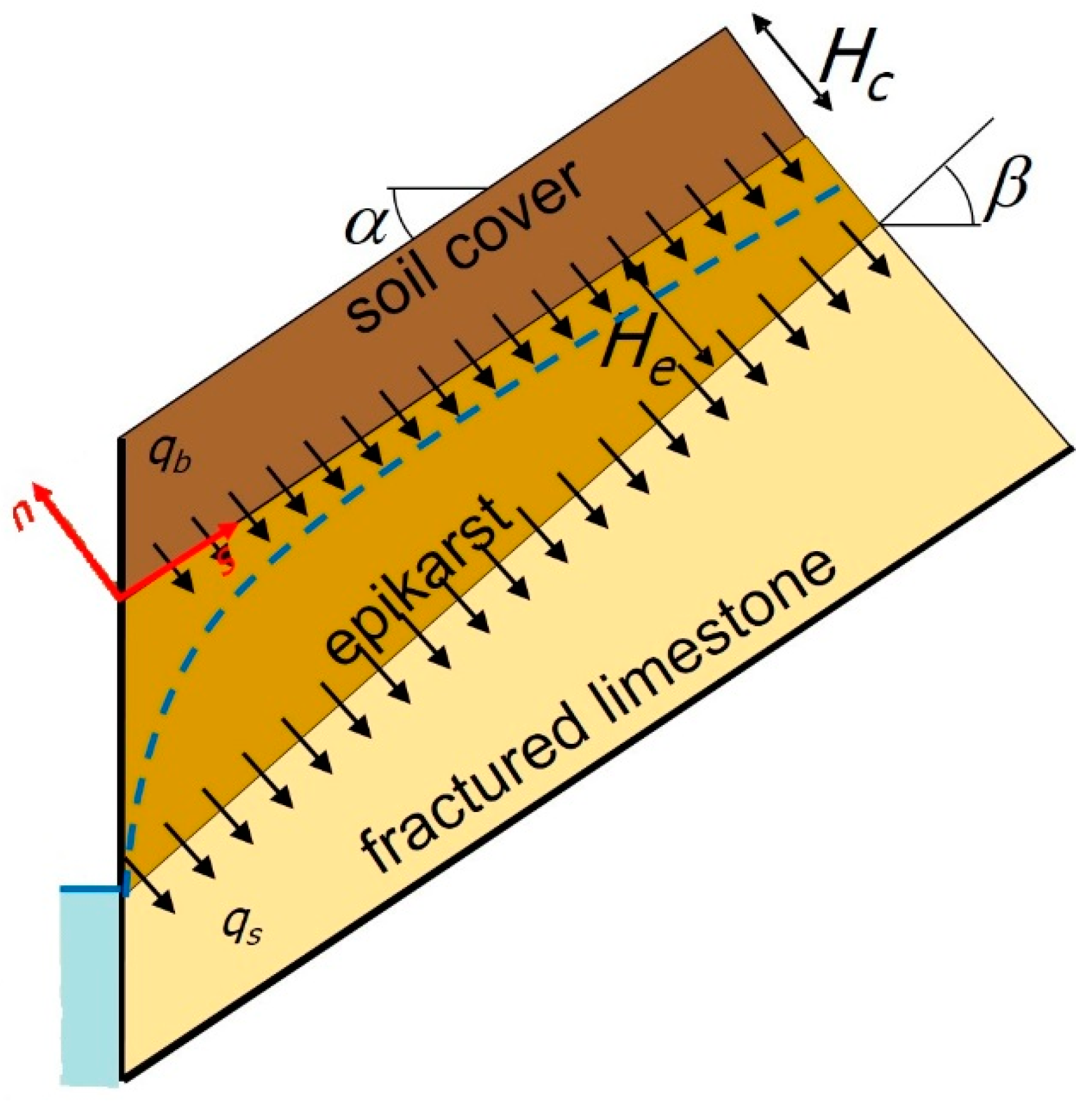
2.2. The Mathematical Model of the Slope

As will be shown in the next section, experimental data from field monitoring suggest that the hydrological regime of the unsaturated soil cover of the slope of Cervinara is affected by the storage of water within the underlying upper part of the limestone fractured bedrock (the epikarst). Hence, a simplified physically based mathematical model of the two interacting hydrological systems (soil cover and epikarst) has been developed. The regular geometry of the slope allows considering a two-dimensional 2D flow field with a constant inclination of the ground surface and constant thickness of the soil cover. The base of the epikarst is assumed to be an inclined plane, too (Figure 3).
The water fluxes through the soil cover, which are supposed as homogeneous for simplicity [33], are modeled with the 2D Richards equation written in the space coordinates s (positive upslope) and n (positive upward), respectively parallel and orthogonal to the slope:
d θ d ψ ψ t = s [ k ( ψ ) ( sin α + ψ s ) ] + n [ k ( ψ ) ( cos α + ψ n ) ] q r
In Equation (1), ψ (L) is soil water potential; θ (−) is soil volumetric water content; α (rad) is the slope inclination angle; θ ( ψ ) represents soil water retention curve; and k ( ψ ) (L/T) represents the hydraulic conductivity function of the soil. The hydraulic characteristic curves of the soil, θ ( ψ ) and k ( ψ ) , are modeled with the van Genuchten–Mualem expressions [34]. The sink term q r (1/T) represents the root water uptake, which evenly distributes the evapotranspiration flux E (L/T) throughout the soil cover according to the local value of water potential [35]:
q r = λ ( ψ ) E ψ > ψ 1 ψ 1 ψ > ψ 2 ψ 2 ψ > ψ 3 ψ ψ 3 λ = ψ / ψ 1 λ = 1 λ = 1 ( ψ ψ 3 ) / ( ψ 2 ψ 3 ) λ = 0
In Equation (2), the parameters ψ 1 = 0.5 m, ψ 2 = 15.0 m, and ψ 3 = 150 m (i.e., the permanent wilting point of the plants) have been assigned according to values suggested in the literature [20,35,36]. The mean potential evapotranspiration flux E of each month is obtained by dividing the values of P E T (L) of Table 1 by the soil cover thickness H c (L) and the duration of the month T m , E = P E T / ( T m H c ) .
At the ground surface ( n = H c ), the infiltration capacity of the soil is calculated according to the current soil water potential value and gradient near the surface. Then, the rainfall intensity excess over the infiltration capacity is turned into overland runoff flow, and the difference is set as infiltration into the soil.
The water level h (L) in the perched aquifer developing in the epikarst has been modeled by assuming the validity of the 1D Darcy equation:
n e h d t = d s [ K e h ( sin β + h d s ) ] + q b q s
In Equation (3), n e (−) is the effective porosity of the epikarst; K e (L/T) is the (saturated) hydraulic conductivity of the epikarst; and β (rad) represents the inclination angle of the epikarst bed. The source and sink terms q b (L/T) and q s (L/T) represent, respectively, the flow crossing the soil–bedrock interface, and the outflow from the epikarst aquifer partly supplying the spring discharge and the deep groundwater recharge. For q s , a simple linear dependence on water level is assumed, while q b is calculated as the flow rate crossing the interface at the base of the soil cover:
q s = K e h L q b = k ( ψ b ) ( cos α + ψ n n = n b ) + d n { θ t n = n b + s [ k ( ψ b ) ( sin α + ψ s | n = n b ) ] }
In Equation (4), L (L) represents the total length of the slope (Figure 3), as it has been assumed as a characteristic length that is suitable for estimating the mean gradient of the outflow from the epikarst; n b (L) represents the coordinate of the soil–bedrock interface in the adopted reference system; and ψ b (L) is the water potential at the base of the soil cover ( n = n b ).
For the soil cover, a no-flow boundary condition has been assumed upslope, and a seepage face boundary conditions has been assumed downslope. For the epikarst aquifer, a free flow condition h / s = 0 has been assumed upslope, and h = 0 , i.e., outflow at atmospheric pressure, has been assumed at the foot of the slope.
Besides the water exchange represented by q b , the two flow fields have been coupled also by introducing the following equation at the soil–bedrock interface, neglecting the water flow through the upper unsaturated part of the epikarst and directly linking the water potential at the base of the soil cover with the water level in the epikarst aquifer:
ψ b = h H e
In Equation (5), H e (L) represents the epikarst thickness, H e = H 0 + s cos α ( sin α sin β ) , with H 0 being the epikarst thickness at the foot of the slope.
The system of differential equations of the model has been numerically solved with a fully implicit finite differences technique. At every time step, an iterative procedure has been implemented, so as to get the coupled solution of Equations (1) and (3). An upwind formulation has been adopted for the first-order spatial derivatives, while centered schemes have been used for the second-order derivatives. The non-linear algebraic system has been iteratively solved with an alternate direction implicit technique. To improve the stability of the numerical solver, water fluxes and hydraulic conductivity have been evaluated on a staggered grid [37].

3. Results and Discussion

In this section, first, some results from field monitoring are reported, which are at the basis of the development of the mathematical model described in Section 2.2, and which give some insight about the choice of the values of the parameters of the model. Then, the results of the application of the model to the simulation of the hydrological response of the slope to actual precipitation records are presented. The obtained results show that the coupled modeling of the unsaturated flow in the soil cover and the perched aquifer developing in the epikarst allows for a realistic simulation of the water potential regime in the soil cover, which is the result of the superposition of long-term seasonal fluctuations and short variations directly related to the sequence of rainfall events and dry intervals.

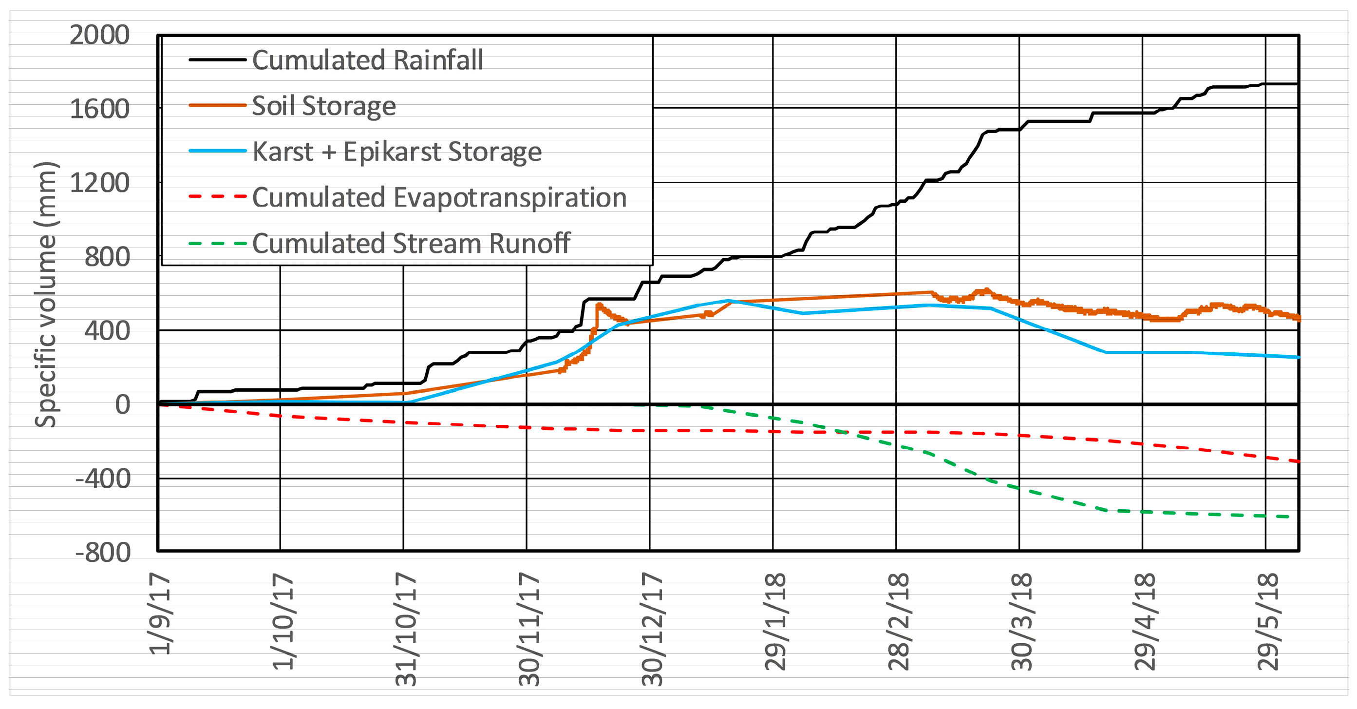
3.1. Slope Water Balance

The hydrometeorological monitoring activities carried out at the slope of Cervinara enable approximately assessing the water balance of the hydrological system consisting of the slope cover, the epikarst, and the deep groundwater system. More specifically, the measurement of rainfall and soil water content at various depths, the estimation of the evapotranspiration based on the measurements of meteorological variables, and the estimation of the water drained by the springs based on the measurements of water level in the streams, have been used to calculate the various terms of the water balance equation between 1 September 2017 and 6 June 2018:
V s + V e + V g = 0 t ( R E q s ) d t
Equation (6) is written in terms of specific storage, i.e., the terms V s , V e and V g (L) on the left-hand side represent, respectively, the water volume stored in a column of unit area of soil, epikarst, and groundwater. The variation of specific storage in time is related, on the right-hand side, to the cumulated difference between rainfall intensity R (L/T), evapotranspiration E (L/T), and specific spring discharge q s (L/T). The overland runoff has been neglected in Equation (6), as it occurs only sporadically, during the highest rainfall intensity peaks, and does not significantly affect the long-term water balance.
The measurements of soil water content θ , provided by the TDR probes installed at the depths of −0.30 m, −0.90 m, −1.40 m, and −2.20 m, allow estimating soil specific storage V s in the entire soil cover, for which a total thickness of 2.60 m was assumed:
V s = θ i Δ z i
In Equation (7), θ i and Δ z i represent the water content recorded by the i-th TDR probe and the soil profile height attributed to that probe, depending on the probe depth, so that Δ z i = H c . The data of only four probes have been used, as the other installed probes experienced several out of order intervals during the considered period.
The water level measurements carried out in the two stream sections plotted in Figure 4, show that only at the end of November 2017 did water start flowing in the downslope stream (Section 1), and that after this date, there was always some discharge in the stream. In Section 2, instead, the establishment of flow was more intermittent. To estimate the stream discharge Q s from the measured water level H (L), a stage–discharge relationship is needed. To establish such a relationship, the cross-sectional area of the stream Section 1 was measured on 22 December 2017, a day with low water level, and on 23 March 2018, when the highest ever observed water level was attained in both streams. On the same days, the flow mean velocity was estimated by timing small wood pieces floating within the stream. The obtained ( H , Q s ) couples were fitted with the following monomial stage–discharge relationship, in which the exponent assigned was equal to 2, so as to be close to the value of the relationship holding for uniform motion in a shallow trapezoidal section:
Q s Q m a x = ( H H m a x ) 2
In Equation (8), H m a x and Q m a x represent, respectively, the maximum measured water level and the corresponding maximum estimated flow discharge. The same relationship has been assumed valid also for the other monitored stream, in which the discharge was estimated only once, on 23 March 2018.
Table 3 summarizes the measured water levels and the corresponding estimated discharges, in the two monitored sections. The obtained stream discharge values should be considered just as a rough estimate, which surely would change if the measurements were carried out with a more sophisticated technique. However, the obtained values are suitable to get a realistic assessment of the water balance of the system. The sum of the two measured discharges was divided by the entire underground watershed extension, which was estimated to be around 2.5 km2 from the hydrogeological map of the area, in order to obtain the specific discharge of the springs draining the epikarst aquifer.
In Figure 4, the estimated trend of the specific storage of Equation (6) is reported. More specifically, as no information about the leakage from the epikarst toward the deep groundwater was available, the terms V e and V g could not be separated, and so only their sum V e + V g could be estimated from the other measured/estimated terms of the balance equation. However, the spring discharge estimated from the stream water level was small, and it would further decrease during summer, when it usually becomes negligible. Hence, it can be argued that the epikarst storage was already very small at the end of the monitoring period, so that the estimated value of around 300 mm is mostly representative of deep groundwater recharge. Such a value is in reasonable agreement with the mean annual regional groundwater recharge estimated in the area [22].
Although the TDR probes were out of order for most of the rainy season, it is clear how the soil storage peaks shortly after the most intense rain storms (e.g., the value of more than 530 mm reached on 7 December), while the variations of storage in the fractured limestone are much smoother. Conversely, the drainage of water from the soil (reduction of soil storage) results were slower than the decrease of limestone storage.

3.2. Estimation of the Parameters of the Slope Model

The parameters of the hydraulic characteristic curves of the van Genuchten–Mualem model had been calibrated in previous studies by back-analysis of field measurements of soil water content and suction [33]. Although a single homogeneous soil layer is assumed, the parameters proved to be able to effectively reproduce the observed trends. The adopted parameters are reported in Table 4.
For the parameters of the epikarst aquifer, namely the effective porosity n e , the epikarst thickness H e , and the hydraulic conductivity K e , the values reported in the literature results were widely spread, owing to the great differences exhibited by karstic systems in terms of density and dimension of fractures, which are affected by climate as well as by rock and soil cover mineralogy. The epikarst thickness is very much related to the characteristics of the soil cover and the yearly precipitation amount [23]. In Mediterranean climate, an epikarst thickness of 10 m was suggested [38]. In a karst aquifer covered by the pyroclastic soil of Campania (very close to the site of Cervinara), epikarst thickness up to 15 m was reported, depending on the soil cover thickness (the thicker the soil cover, the thicker the epikarst) and on vegetation cover (thicker epikarst under woodlands, thinner under grasslands) [26]. For simplicity, a constant thickness H e = 14   m was assumed. For K e , values between 10−7 m/s and 10−3 m/s have been suggested e.g., Freeze and Cherry [39], and such a wide interval was confirmed by more recent studies e.g., White, Worthington, Allocca et al., Binet et al. [40,41,42,43]. For n e , the reported values range from less than 1% [44] up to 7% [29,45]. In this study, the values of n e and K e have been chosen so that in an 11-year long simulation with real rainfall records, the perched aquifer resulted in dynamic equilibrium (i.e., it returned nearly to the same water level at the end of every hydrological year, with seasonal fluctuations consistent with the typical observed water potential regime of the overlying soil cover). The results of these simulations, which are given in the next subsection, led to the assumption of n e = 1.5 % and K e = 1.1 × 10 6 m/s.

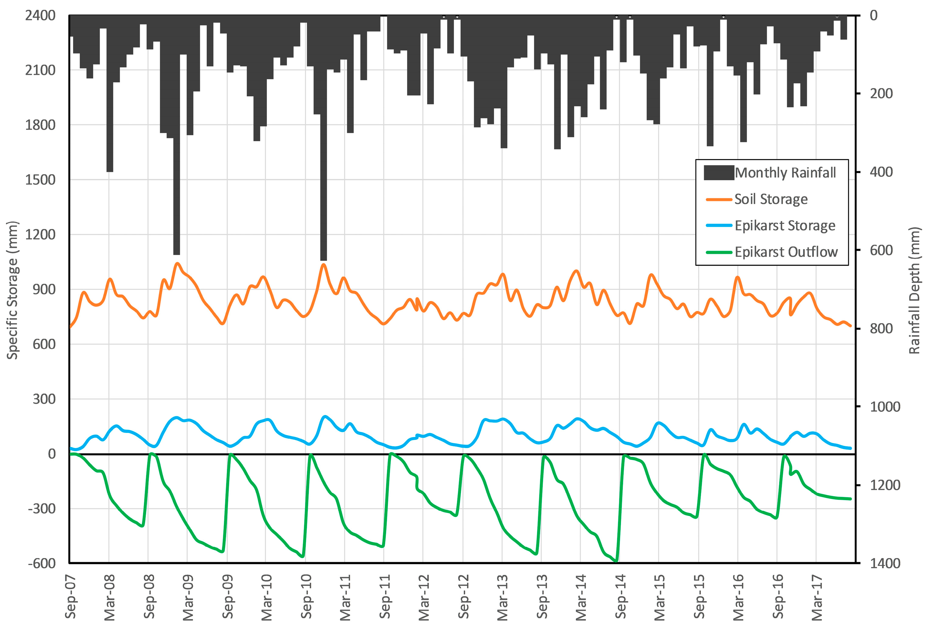
3.3. Long-Term Simulations

The coupled model has been applied to the simulation of the response of the slope to precipitations from 1 September 2006 to 31 August 2017. For this simulation, the rainfall height series with a sampling interval of 10 min, recorded by the rain gauge of Cervinara of the meteorological alert network of the Civil Protection Agency of Campania, has been used. Table 5 summarizes the yearly precipitation depths of the series. The initial conditions on 1 September 2006 have been set by running a two-year long simulation with the precipitation record of 2013–2014 rescaled to have a total yearly precipitation that is equal to the yearly mean value (1613 mm).
Figure 5 reports the predicted trends of soil storage, epikarst aquifer water level, and yearly cumulated epikarst outflow during the entire simulation period. The monthly precipitation histogram is also plotted. It looks clear how the aquifer fluctuations are affected by the seasonal precipitation amount, especially in spring, when the evapotranspiration subtracts a significant water amount from the soil cover (Table 2). The trends predicted in all of the years resemble those observed in 2017–2018, confirming that the model is capable of reliably reproducing the actual response of the slope. The predicted fluctuations of soil storage correspond to the mean volumetric water content in the cover between 0.3 and 0.5. The fluctuations of epikarst storage correspond to soil water potential at the base of the cover, oscillating between −12.0 m to −14.0 m in summer, and −1.0 m to −3.0 m in winter. Both the modeled seasonal trends of soil water potential and water content result in good agreement with field observations available for similar slopes e.g.,Napolitano et al., Cascini et al., Comegna et al. [4,9,10].
It is interesting to note the different response time to precipitations of epikarst storage, which shows a smooth behavior, compared to soil storage, the graph of which is characterized by abrupt peaks following rainy periods. The effects of potentially triggering events (heavy rain storms) are clearly distinguishable from those of the hydrological predisposing cause, which are represented by the seasonal soil moisture fluctuations related to the water level in the aquifer. It becomes clear why in some cases (e.g., 2008–2009 and 2010–2011), although the occurred long-lasting precipitations (in both years, monthly precipitation higher than 600 mm was recorded) led to unusual filling of the epikarst aquifer, this predisposing condition did not result in any landslide triggering. In fact, during the periods of maximum water level in the aquifer, none of the occurred rain storms was large enough to cause a significant increase of soil storage, i.e., the infiltration rate was nearly compensated by the leakage towards the aquifer. The maximum soil storage values—slightly higher than 1000 mm—were attained in January 2009, November 2010, and February 2014, and correspond to a mean water content in the profile of about 0.5, which is still far from saturation.

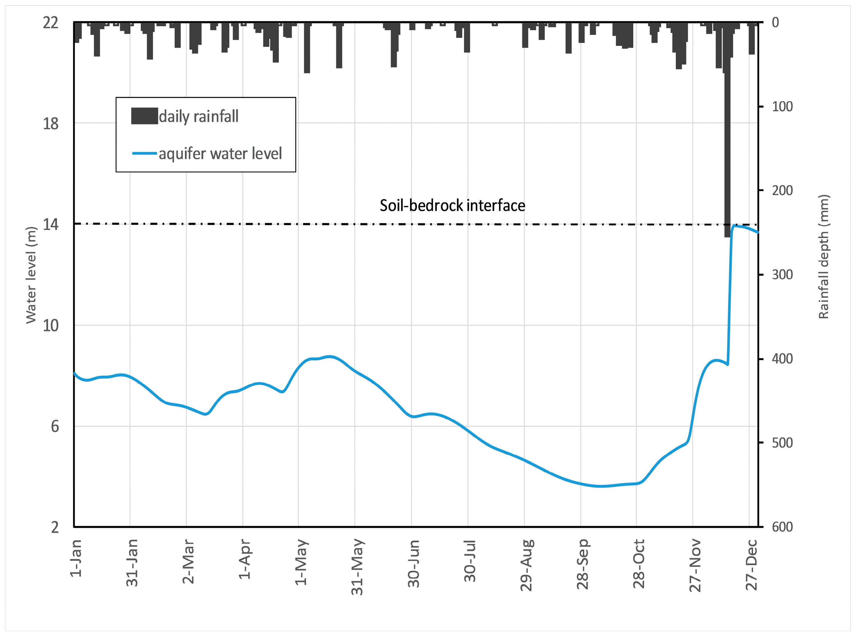
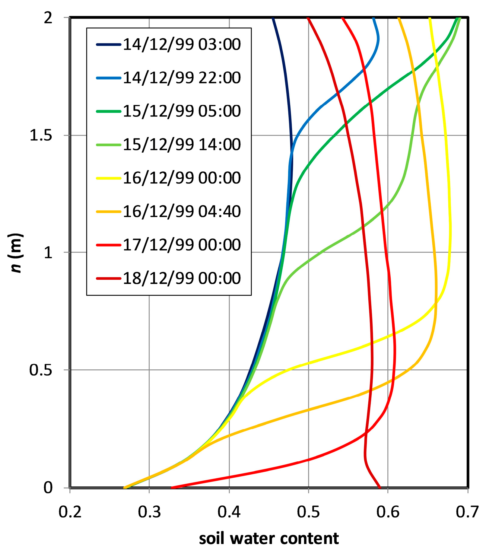
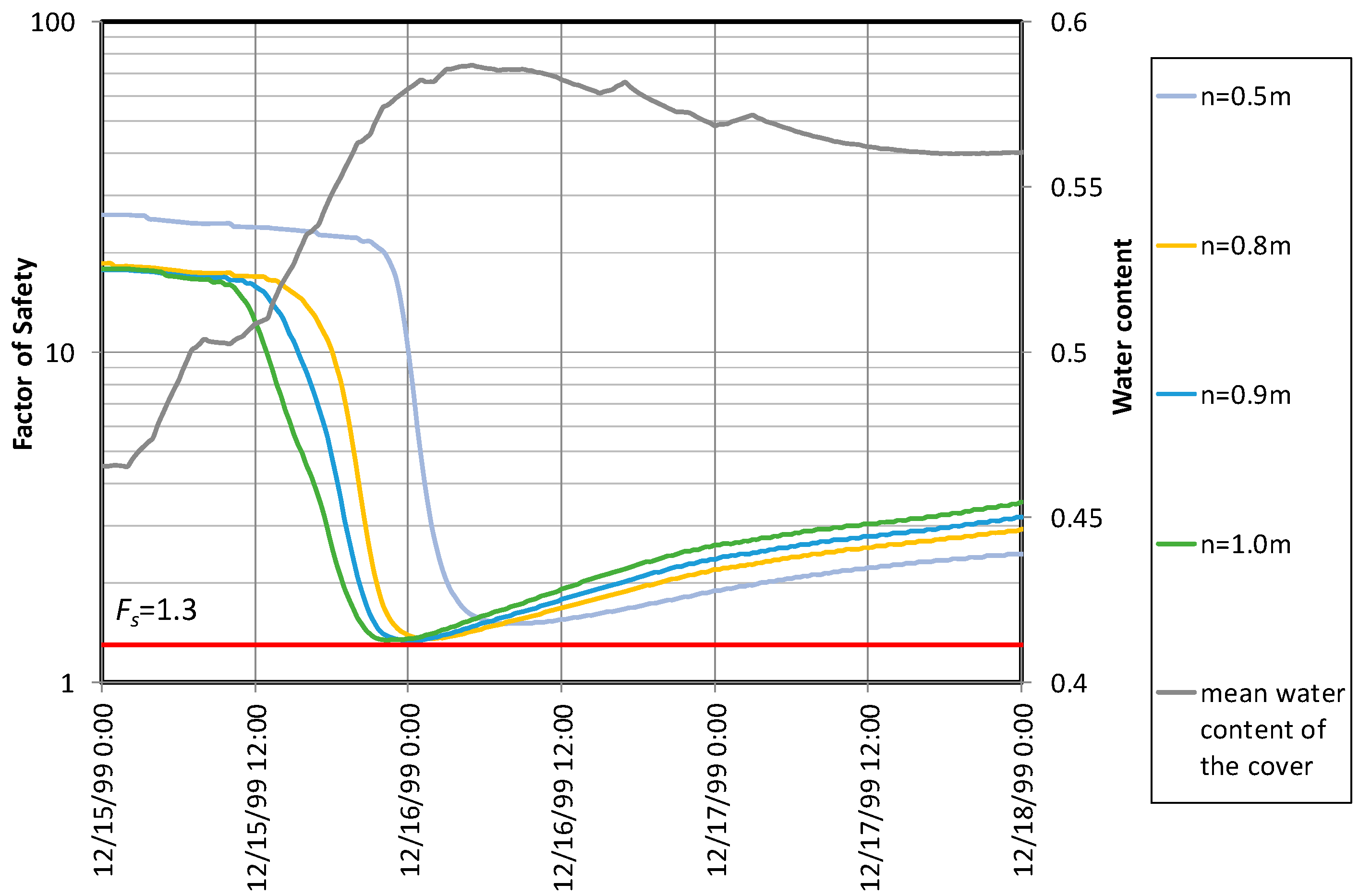
3.4. Simulation of Year 1999

The importance of the predisposing conditions induced in the soil by the high water level developing in the underlying epikarst aquifer is confirmed by the results of the simulation of the year 1999. The total yearly precipitation depth was 1807 mm, i.e., not very high, although larger than the average. However, a landslide was triggered along the slope in the early morning of 16 December, after a rain storm of about 325 mm in 50 h. The initial conditions at the beginning of the year have been assigned, in terms of soil water potential and aquifer water level, by taking the average of the values, obtained on 1 January at 0:00, of all 11 years considered for the long-term simulations (i.e., from 2007 to 2017).
Figure 6 reports the predicted time history of the water level in the aquifer, together with the daily hyetograph, for the whole year 1999. It looks clear that during the first half of the year, the predicted aquifer water level remained always at least 5 m below the soil–bedrock interface, so that dry conditions at the base of the soil column were present during the entire period. Nonetheless, after the typical summer decrease, which led between 10–13 October to ψ b < 10   m at the depth of −2.0 m, during the following period of frequent precipitations (412 mm in less than two months, between 15 October and 13 December), the aquifer level rose nearly 5 m. In the same period, the mean soil water content grew only from 0.39 to 0.46. Hence, the process of water level build-up in the perched aquifer, developing in about two months, represents the hydrological cause that created the predisposing conditions for the slope failure. The triggering event consisted of nearly 325 mm of rainfall fallen in 48 h, between 6 a.m. on 14 December and the same hour on 16 December. Such a rain storm effectively induced slope failure thanks to the existence of the predisposing conditions.
In fact, in an unsaturated cohesionless shallow cover characterized by an inclination angle close to the friction angle as the considered case, the triggering of a landslide requires the attainment of a nearly saturated condition. In fact, under the infinite slope hypothesis, which can be assumed valid for a large part of the considered slope, the safety factor assumes the following expression:
F S = τ l i m τ α = c + ( σ α u a ) tan ϕ + ( u a u w ) χ tan ϕ γ ( H c n ) sin α cos α
In Equation (9), σ α and τ α represent, respectively, normal and shear stress components acting along a plane parallel to the slope; u w and u a are pore water and air pressure (the latter assumed as equal to atmospheric pressure); χ is the Bishop coefficient, which was introduced to calculate the contribution of soil suction to the shear strength of an unsaturated soil, and is related to the degree of saturation of the soil e.g., Greco and Gargano, Lu et al. [16,46]; γ is the mean specific weight of the soil layer between the ground surface and the depth H c n . As it is ( σ α u a ) = γ ( H c n ) ( cos α ) 2 , in a soil with c = 0 , similar to the ashes of Cervinara, the vanishing of suction implies that for α ϕ , it results F S 1 , i.e., landslide-triggering conditions.
Given the high porosity of the considered deposit and the typical soil water storage during the wet season rarely exceeding a mean water content of 0.5, a large water volume has to be stored in the deposit to approach saturation, which is namely about 500 mm for the considered soil cover thickness of 2.0 m. As the triggering rainfall depth was “only” about 325 mm, this implies that saturation was reached only locally within the soil cover, and that the drainage from the soil cover during the triggering event was ineffective.
When the water level in the aquifer is high, the water potential gradient required for the establishment of an intense flow rate q b through the soil–bedrock interface may lead to soil saturation (suction vanishing), and consequently to the triggering of a landslide along a slope with an inclination angle close to the soil effective friction angle, as the considered slope.
Figure 7 reports the volumetric water content profiles throughout the soil cover that were simulated at various times between 14–18 December. It appears clear how with the given initial conditions, the intense infiltration led to the establishment of a high soil moisture gradient at the base of the cover, so that most of the infiltrating water remained stored in the upper 1.5 m until the early morning of 16 December. This is due to the dry state of the soil at the base of the cover before the triggering event (i.e., θ 0.26 , corresponding to ψ b 5   m ) caused by the relatively low water level in the perched aquifer. With the low unsaturated hydraulic conductivity of such a dry soil layer, only under large water potential gradient water could penetrate the base of the cover and cross the soil–bedrock interface. Through the soil water retention curve, large water potential gradients correspond to large soil moisture gradients. The simulated soil moisture profiles show that the maximum soil moisture gradient at the base of the cover developed on 16 December, between midnight and 5 am (which was the actual triggering time), leading to water content as high as 0.68 between 1.0–1.3 m below the ground surface. As said, the attainment of this value is related not only to the characteristics of the triggering rainfall event, but also to the initial soil moisture profile and to the water content at the soil–bedrock interface, which in turn depend on the water level in the epikarst aquifer. Both these latter features are the result of the predisposing hydrological phase.
The effect of the infiltration features on the potential triggering of a landslide is shown in Figure 8, which reports the predicted evolution of the factor of safety at various depths, as well as the trend of the mean water content of the soil cover during the triggering event. The worst conditions for slope stability are predicted around midnight on 16 December, when F S 1.3 was attained at depths between 1.0–1.5 m below the soil surface (respectively, n = 1.0   m and n = 0.5   m ). Such depth is consistent with the reported depth of the failure surface, which was well above the interface with the bedrock [47]. Although the predicted minimum value of F S would not imply slope failure, it is small enough to be considered indicative of potential instability. In fact, heterogeneities play a big role in the triggering of landslides, which cannot be completely captured by the simplified modeling approach adopted here. The real slope presents variable inclination, soil cover thickness, and hydraulic and geotechnical soil properties. Furthermore, the considered cover, which is here schematized for simplicity as homogeneous, is actually characterized by soil layers with different properties (Table 1). The presence of layers with low hydraulic conductivity may exacerbate the mechanism suggested by the modeling results, enhancing the moisture gradient required for the infiltrating water to reach the soil–bedrock interface. This would lead to higher water content within the soil profile, and consequently to a smaller factor of safety. Indeed, it has been recently shown that in the pyroclastic covers of Campania, either coarse layers (i.e., pumices) in dry conditions, or fine layers (i.e., weathered ashes) in wet conditions may hinder the infiltration process [8]. Although the detailed description of the infiltration process falls beyond the aim of this simplified approach, the model results shed some light on the concurrence of long-term predisposing processes and short triggering mechanisms for landslide initiation.

4. Conclusions

The triggering of rainfall-induced landslides in shallow soil covers depends on the characteristics of the triggering rainfall, as well as on the soil moisture conditions at the onset of the event. In this paper, the seasonal dynamics of soil moisture typically observed in the slopes of Campania (southern Italy), which were characterized by shallow pyroclastic covers laying upon a fractured and karstified limestone bedrock, is linked to the fluctuations of the water level in a perched aquifer located in the upper part of the bedrock (epikarst). A simplified physically-based mathematical model of the coupled interaction between the unsaturated flows within the soil cover and the saturated flow in the aquifer is proposed. The parameters describing the hydraulic properties of the soil cover are chosen based on the results of previous laboratory and field investigations. The hydraulic parameters of the epikarst aquifer are assigned according to literature indications, and to the results of currently ongoing field monitoring.
The model has been applied to simulate the hydrological response to precipitations of the slope of Cervinara (about 40 km NE of Naples). The simulation results of the period 2006–2017 show that the model is capable of realistically reproducing the typical seasonal soil moisture trends observed in the area. The model clearly identifies the different response times to precipitations of the soil cover storage, which are rapidly affected by rainy days, and of the perched epikarst aquifer water level, which changes in response to precipitations at a monthly scale. This allows the distinction between the predisposing causes of landslides, i.e., the relatively slow processes of accumulation of water in the perched epikarst aquifer (and its effects on the hydraulic behavior of the soil–bedrock interface), and the triggers, which are represented by single intense rain storms that are too short for allowing effective drainage from the slope cover. The identified cause–trigger interplay offers a sound and convincing interpretation of the landslide that occurred on 16 December 1999.

Author Contributions

All the Authors contributed to the development of the research idea, to the monitoring activities, to the conceivement of the paper, and to the discussion and comment of the results; G.F.S. and P.M. carried out the numerical experiments; E.D. carried out the geotechnical analyses; R.G. developed the mathematical model and wrote the paper, which was commented and edited by all the others.

Funding

This research is part of the Ph.D. project “Modeling of hydrological processes leading to landslides in pyroclastic granular covers, for the development of early warning systems” within the Doctoral Course A.D.I. of Università degli Studi della Campania, ‘L. Vanvitelli’, supported by funds of Università degli Studi della Campania, ‘L. Vanvitelli’.

Acknowledgments

The authors acknowledge the Civil Protection Agency of Campania Region for providing the rainfall data.

Conflicts of Interest

The authors declare no conflict of interest.

References

  1. Crozier, M.J. Prediction of rainfall-triggered landslides: A test of the antecedent water status model. Earth Surf. Process. Landf. 1999, 24, 825–833. [Google Scholar] [CrossRef]
  2. Rahimi, A.; Rahardjo, H.; Leong, E.C. Effect of Antecedent Rainfall Patterns on Rainfall-Induced Slope Failure. J. Geotech. Geoenviron. Eng. 2011, 137. [Google Scholar] [CrossRef]
  3. Von Ruette, J.; Lehmann, P.; Or, D. Effects of rainfall spatial variability and intermittency on shallow landslide triggering patterns at a catchment scale. Water Resour. Res. 2014, 50, 7780–7799. [Google Scholar] [CrossRef] [Green Version]
  4. Napolitano, E.; Fusco, F.; Baum, R.L.; Godt, J.W.; De Vita, P. Effect of antecedent-hydrological conditions on rainfall triggering of debris flows in ash-fall pyroclastic mantled slopes of Campania (southern Italy). Landslides 2016, 13, 967–983. [Google Scholar] [CrossRef]
  5. Bogaard, T.A.; Greco, R. Landslide hydrology: From hydrology to pore pressure. Wiley Interdiscip. Rev. Water 2016, 3, 439–459. [Google Scholar] [CrossRef]
  6. Tromp-van Meerveld, H.J.; McDonnell, J.J. Threshold relations in subsurface stormflow: 2. The fill and spill hypothesis. Water Resour. Res. 2006, 42, W02411. [Google Scholar] [CrossRef]
  7. Nieber, J.L.; Sidle, R.C. How do disconnected macropores in sloping soils facilitate preferential flow? Hydrol. Process. 2010, 24, 1582–1594. [Google Scholar] [CrossRef]
  8. Damiano, E.; Greco, R.; Guida, A.; Olivares, L.; Picarelli, L. Investigation on rainwater infiltration into layered shallow covers in pyroclastic soils and its effect on slope stability. Eng. Geol. 2017, 220, 208–218. [Google Scholar] [CrossRef]
  9. Cascini, L.; Sorbino, G.; Cuom, O.S.; Ferlisi, S. Seasonal effects of rainfall on the shallow pyroclastic deposits of the Campania region (southern Italy). Landslides 2014, 11, 779–792. [Google Scholar] [CrossRef]
  10. Comegna, L.; Damiano, E.; Greco, R.; Guida, A.; Olivares, L.; Picarelli, L. Field hydrological monitoring of a sloping shallow pyroclastic deposit. Can. Geotech. J. 2016, 53, 1125–1137. [Google Scholar] [CrossRef] [Green Version]
  11. Glade, T.; Crozier, M.; Smith, P. Applying probability determination to refine landslide-triggering rainfall thresholds using an empirical “antecedent daily rainfall model”. Pure Appl. Geophys. 2000, 157, 1059–1079. [Google Scholar] [CrossRef]
  12. Chleborad, A.F.; Baum, R.L.; Godt, J.W.; Powers, P.S. A prototype for forecasting landslides in the Seattle, Washington, Area. Rev. Eng. Geol. 2008, 20, 103–120. [Google Scholar] [CrossRef]
  13. Bogaard, T.A.; Greco, R. Invited perspectives: Hydrological perspectives on precipitation intensity-duration thresholds for landslide initiation: Proposing hydro-meteorological thresholds. Nat. Hazards Earth Syst. Sci. 2018, 18, 31–39. [Google Scholar] [CrossRef]
  14. Picarelli, L.; Damiano, E.; Greco, R.; Minardo, A.; Olivares, L.; Zeni, L. Performance of slope beahviour indicators in unsaturated pyroclastic soils. J. Mt. Sci. 2015, 12, 1434–1447. [Google Scholar] [CrossRef]
  15. Lu, N.; Likos, W.J. Suction stress characteristic curve for unsaturated soil. J. Geotech. Geoenviron. Eng. 2006, 132, 131–142. [Google Scholar] [CrossRef]
  16. Greco, R.; Gargano, R. A novel equation for determining the suction stress of unsaturated soils from the water retention curve based on wetted surface area in pores. Water Resour. Res. 2015, 51, 6143–6155. [Google Scholar] [CrossRef] [Green Version]
  17. Olivares, L.; Picarelli, L. Shallow flowslides triggered by intense rainfalls on natural slopes covered by loose unsaturated pyroclastic soils. Geotechnique 2003, 53, 283–288. [Google Scholar] [CrossRef]
  18. Damiano, E.; Olivares, L.; Picarelli, L. Steep-slope monitoring in unsaturated pyroclastic soils. Eng. Geol. 2012, 137–138, 1–12. [Google Scholar] [CrossRef]
  19. Reder, A.; Pagano, L.; Picarelli, L.; Rianna, G. The role of the lowermost boundary conditions in the hydrological response of shallow sloping covers. Landslides 2017, 14, 861–873. [Google Scholar] [CrossRef]
  20. Greco, R.; Comegna, L.; Damiano, E.; Guida, A.; Olivares, L.; Picarelli, L. Conceptual hydrological modeling of the soil-bedrock interface at the bottom of the pyroclastic cover of Cervinara (Italy). Procedia Earth Plan. Sci. 2014, 9, 122–131. [Google Scholar] [CrossRef]
  21. Cascini, L.; Cuomo, S.; Guida, D. Typical source areas of May 1998 flow-like mass movements in the Campania region, Southern Italy. Eng. Geol. 2008, 96, 107–125. [Google Scholar] [CrossRef]
  22. Allocca, V.; Manna, F.; De Vita, P. Estimating annual groundwater recharge coefficient for karst aquifers of the southern Apennines (Italy). Hydrol. Earth Syst. Sci. 2014, 18, 803–817. [Google Scholar] [CrossRef] [Green Version]
  23. Bakalowicz, M. Epikarst. In Encyclopedia of Caves, 2nd ed.; White, W.B., Culver, D.C., Eds.; Academic Press: London, UK, 2012; pp. 284–288. ISBN 9780123838339. [Google Scholar]
  24. Perrin, J.; Jeannin, P.-Y.; Zwahlen, F. Epikarst storage in a karst aquifer: A conceptual model based on isotopic data, Milandre test site, Switzerland. J. Hydrol. 2003, 279, 106–124. [Google Scholar] [CrossRef]
  25. Hartmann, A.; Goldscheider, N.; Wagener, T.; Lange, J.; Weiler, M. Karst water resources in a changing world: Review of hydrological modeling approaches. Rev. Geophys. 2014, 52, 218–242. [Google Scholar] [CrossRef]
  26. Celico, F.; Naclerio, G.; Bucci, A.; Nerone, V.; Capuano, P.; Carcione, M.; Allocca, V.; Celico, P. Influence of pyroclastic soil on epikarst formation: A test study in southern Italy. Terra Nova 2010, 22, 110–115. [Google Scholar] [CrossRef] [Green Version]
  27. Petrella, E.; Capuano, P.; Carcione, M.; Celico, F. A high altitude temporary spring in a compartmentalized carbonate aquifer: The role of low-permeability faults and karst conduits. Hydrol. Process. 2009, 23, 3354–3364. [Google Scholar] [CrossRef]
  28. Jukic, D.; Denic-Jukic, V. Groundwater balance estimation in karst by using a conceptual rainfall–runoff model. J. Hydrol. 2009, 373, 302–315. [Google Scholar] [CrossRef]
  29. Fu, Z.; Chen, H.; Xu, Q.; Jia, J.; Wang, S.; Wang, K. Role of epikarst in near-surface hydrological processes in a soil mantled subtropical dolomite karst slope: Implications of field rainfall simulation experiments. Hydrol. Process. 2016, 30, 795–811. [Google Scholar] [CrossRef]
  30. Xu, X.; Huang, G.; Zhan, H.; Qu, Z.; Huang, Q. Integration of SWAP and MODFLOW-2000 for modeling groundwater dynamics in shallow water table areas. J. Hydrol. 2012, 412, 170–181. [Google Scholar] [CrossRef]
  31. Szymkiewicz, A.; Gumuła-Kawęcka, A.; Šimůnek, J.; Leterme, B.; Beegum, S.; Jaworska-Szulc, B.; Pruszkowska-Cacers, M.; Gorczewska-Langner, W.; Angulo-Jaramillo, R.; Jacques, D. Simulations of freshwater lens recharge and salt/freshwater interfaces using the HYDRUS and SWI2 packages for MODFLOW. J. Hydrol. Hydromech. 2018, 66, 246–256. [Google Scholar] [CrossRef] [Green Version]
  32. Shuttleworth, W.J. Evaporation. In Handbook of Hydrology; Maidment, D.R., Ed.; McGraw-Hill: New York, NY, USA, 1993; pp. 4.1–4.53. ISBN 0070397325. [Google Scholar]
  33. Greco, R.; Comegna, L.; Damiano, E.; Guida, A.; Olivares, L.; Picarelli, L. Hydrological modelling of a slope covered with shallow pyroclastic deposits from field monitoring data. Hydrol. Earth Syst. Sci. 2013, 17, 4001–4013. [Google Scholar] [CrossRef] [Green Version]
  34. Van Genuchten, M.T. A closed-form equation for predicting the hydraulic conductivity of unsaturated soils. Soil Sci. Soc. Am. J. 1980, 44, 892–898. [Google Scholar] [CrossRef]
  35. Feddes, R.A.; Kowalik, P.; Kolinska-Malinka, K.; Zaradny, H. Simulation of field water uptake by plants using a soil water dependent root extraction function. J. Hydrol. 1976, 31, 13–26. [Google Scholar] [CrossRef]
  36. Nyambayo, V.P.; Potts, D.M. Numerical simulation of evapotranspiration using a root water uptake model. Comput. Geotech. 2010, 37, 175–186. [Google Scholar] [CrossRef]
  37. Peyret, R.; Taylor, T.D. Computational Methods for Fluid Flow; Springer: New York, NY, USA, 1983; p. 358. ISBN 978-3-642-85952-6. [Google Scholar]
  38. Al-Fares, W.; Bakalowicz, M.; Guérin, R.; Dukhan, M. Analysis of the karst aquifer structure by means of a Ground Penetrating Radar (GPR). Example of the Lamalou area (Hérault, France). J. Appl. Geophys. 2002, 51, 97–106. [Google Scholar] [CrossRef]
  39. Freeze, R.A.; Cherry, J.A. Groundwater; Prentice-Hall: Englewood Cliffs, NJ, USA, 1979; p. 604. [Google Scholar]
  40. White, W.B. A brief history of karst hydrogeology: Contributions of the NSS. J. Cave Karst. Stud. 2007, 69, 13–26. [Google Scholar]
  41. Worthington, S.R.H. Diagnostic hydrogeologic characteristics of a karst aquifer Kentucky, (USA). Hydrogeol. J. 2009, 17, 1665–1678. [Google Scholar] [CrossRef]
  42. Allocca, V.; De Vita, P.; Manna, F.; Nimmo, J.R. Groundwater recharge assessment at local and episodic scale in a soil mantled perched karst aquifer in southern Italy. J. Hydrol. 2015, 529, 843–853. [Google Scholar] [CrossRef]
  43. Binet, S.; Joigneaux, E.; Pauwels, H.; Albéric, P.; Fléhoc Ch Bruand, A. Water exchange, mixing and transient storage between a saturated karstic conduit and the surrounding aquifer: Groundwater flow modeling and inputs from stable water isotopes. J. Hydrol. 2017, 544, 278–289. [Google Scholar] [CrossRef] [Green Version]
  44. Ladouche, B.; Marechal, J.C.; Dorfliger, N. Semi-distributed lumped model of a karst system under active management. J. Hydrol. 2014, 509, 215–230. [Google Scholar] [CrossRef]
  45. Zhang, Z.; Chen, X.; Chen, X.; Shi, P. Quantifying time lag of epikarst-spring hydrograph response to rainfall using correlation and spectral analyses. Hydrogeol. J. 2013, 21, 1619–1631. [Google Scholar] [CrossRef]
  46. Lu, N.; Godt, J.W.; Wu, D.T. A closed-form equation for effective stress in unsaturated soil. Water Resour. Res. 2010, 46, W05515. [Google Scholar] [CrossRef]
  47. Fiorillo, F.; Guadagno, F.M.; Equino, S.; De Blasio, A. The December 1999 Cervinara landslides: Further debris flows in the pyroclastic deposits of Campania (southern Italy). Bull. Eng. Geol. Environ. 2001, 60, 171–184. [Google Scholar] [CrossRef]
Figure 1. The slope of Cervinara: geographic location (a); front view of the scarp of the main landslide of 16 December 1999 (b); cross-section sketch with indication of the monitoring station and of the layered profile observed in four pits (c).
Water 10 00948 g001
Figure 2. Hydrogeological map of the slope of Cervinara, with indication of the monitoring station, the main springs, and the scarp of the main landslide of 16 December 1999.
Water 10 00948 g002
Figure 3. Sketch of the flow domains of the coupled mathematical model of unsaturated soil cover and epikarst aquifer. The dashed blue line qualitatively represents the water table of the perched epikarst aquifer.
Water 10 00948 g003
Figure 4. Specific water balance of the slope, estimated from field monitoring data between 1 September 2017 and 6 June 2018.
Water 10 00948 g004
Figure 5. Specific water balance of the slope, estimated by means of the model, from 1 September 2017 till 6 June 2018.
Water 10 00948 g005
Figure 6. Daily hyetograph and simulated epikarst aquifer water level during 1999.
Water 10 00948 g006
Figure 7. Simulated soil water content profiles throughout the soil cover (calculated at s = 150   m as representative of most of the slope length) between 14–18 December 1999.
Water 10 00948 g007
Figure 8. Predicted factor of safety F S at various depths (calculated at s = 150   m as representative of most of the slope length), and mean water content of the soil cover, between 15–17 December 1999, when a landslide occurred at Cervinara.
Water 10 00948 g008
Table 1. Main physical characteristics of the pyroclastic soils of the cover of Cervinara (n, total porosity; γdry, dry unit weight; Ksat, saturated hydraulic conductivity; ф’, effective friction angle; c’, effective cohesion).
SoilClay %Silt %Sand %Gravel %n (%)γdry (kN/m3)Ksat (m/s)ф’ (°)c’ (kPa)
coarse pumices00–448–6038–5650–551.2–1.35 × 10⁻⁶–1 × 10⁻⁵--
ashes2–54–1475–850–870–750.7–0.81 × 10⁻⁶–6 × 10−6380
fine pumices0–42–1555–6025–4050–551.2–1.3---
weathered ashes2–1010–4040–802–860–650.9–1.08 × 10⁻⁷–1 × 10−63111
Table 2. Mean potential evapotranspiration ( P E T (L)), calculated with the empirical formula of Thornthwaite, and precipitation depth (L), based on meteorological data measured at Cervinara between 2001 and 2017.
Period P E T   ( mm )   at   320   m   a . s . l . P E T   ( mm )   at   760   m   a . s . l . Mean Precipitation Depth (mm)
January1410226
February1612168
March3126201
April5145127
May857687
June12110771
July14512754
August13511843
September988694
October6457124
November3026214
December1714193
Year8087031602
Table 3. Measured water levels, estimated flow discharges in the two monitored stream sections, and estimated specific spring discharge from the whole drained area. Bold values represent discharge estimated by measuring the cross-sectional area and estimating the mean flow velocity. The other discharge values are obtained by means of Equation (8).
Measurement DateSection 1Section 2 q s   ( mm / h )
H   ( cm ) Q s   ( L / s ) H   ( cm ) Q s   ( L / s )
7 December 20170.00.00.00.00.0
12 December 20172.00.20.00.00.0
22 December 201711.013.80.00.01.7
11 January 201814.025.30.00.03.1
18 January 201828.0143.17.07.418.7
5 February 201818.047.40.00.05.9
8 March 201835.0250.010.018.133.4
23 March 201835.0250.015.050.037.3
20 April 201815.030.10.00.03.7
11 May 201814.025.30.00.03.1
6 June 201812.519.10.00.02.4
Table 4. Parameters of the coupled mathematical model of unsaturated soil cover and epikarst aquifer.
Soil coverCover thickness, H c (m)2.0
Slope length (m)200
Saturated water content, θ s a t (−)0.75
Residual water content, θ r e s (−)0.01
Air entry point, α v G (m−1)6.0
Van Genuchten retention curve shape parameter, n v G (−)1.1
Saturated hydraulic conductivity, k s a t (m/s)3.0 × 10−5
EpikarstEpikarst thickness, H e (m)14
Effective porosity, n e (−)0.015
Epikarst hydraulic conductivity, K e (m/s)1.1 × 10−6
Table 5. Annual precipitations recorded by the rain gauge of Cervinara of the meteorological alert network of the Civil Protection Agency of Campania. Every year begins on 1 September and ends on 31 August.
YearAnnual Rainfall Height (mm)
2006–20071235
2007–20081431
2008–20092119
2009–20101739
2010–20111928
2011–20121122
2012–20132129
2013–20142000
2014–20151427
2015–20161524
2016–20171090
Mean1613

