Best Fit and Selection of Theoretical Flood Frequency Distributions Based on Different Runoff Generation Mechanisms

Abstract

Theoretically derived distributions allow the detection of dominant runoff generation mechanisms as key signatures of hydrologic similarity. We used two theoretically derived distributions of flood peak annual maxima: the first is the “IF” distribution, which exploits the variable source area concept, coupled with a runoff threshold having scaling properties; the second is the Two Component-IF (TCIF) distribution, which generalizes the IF distribution, and is based on two different threshold mechanisms, associated with ordinary and extraordinary events, respectively. By focusing on the application of both models to two river basins, of sub-humid and semi-arid climate in Southern Italy, we present an ad hoc procedure for the estimation of parameters and we discuss the use of appropriate techniques for model selection, in the case of nested distributions.

1. Introduction

The identification of dominant processes in flood generation represents the main route for building models able to reproduce real processes and reduce the uncertainty of flood prediction with particular reference to ungauged basins. In this context, the detection of the dynamics responsible for runoff generation and the suitability of a given conceptual scheme may provide interesting insights into basin classification and regionalization.

With this aim, in the recent past, much effort has been spent by hydrologists in order to maximize the exploitation of different kinds of information useful for understanding the hydrological regimes. Basically, in the framework of flood frequency analysis, the uncertainty of prediction is strongly affected by the scarcity of historical data usually due to poor quality or quantity in peak discharge time series. One of the most popular strategies for coping with data scarcity is provided by regional analysis whose purpose is to transfer hydrological information from gauged to ungauged watersheds by identifying hydrologically homogeneous regions and allowing for improved predictions in ungauged basins [1].

In the last few years many studies have been devoted to the analysis of spatial variability in soil properties and land use. They investigate relationships between basin physical properties, model parameters and hydrological response (assuming that catchments with the same physical characteristics have similar hydrological response) with the aim of finding basin descriptors representative of hydrological signatures (e.g., [2,3,4,5,6,7,8]). Others particularly focus on the issue of prediction in ungauged basins [9,10,11,12,13].

Notwithstanding the availability of numerous studies in this field, today no clear guidance is available regarding which model or model structure is appropriate for any particular catchment or management question. Similarly, no clear guidance is available regarding which dominant processes and mechanisms are operating in a given catchment type [14].

A promising opportunity for hydrologists arises from the introduction of physical concepts in the construction of the flood frequency curve by means of derived distributions (e.g., [15,16,17,18,19,20,21]). These models, with a simple and physically consistent structure, may provide a valuable compromise between the complexity of real processes and the need for model consistency. In this context, several authors (e.g., [22,23,24]) have explored the effects due to the coexistence of different runoff processes in flood generation. For instance, Sivapalan et al. [22] assumed that floods may be produced by both infiltration excess and saturation excess in the same basin. Another case of coexistence of different runoff processes is given by Allamano et al. [24] who proposed a distribution where runoff includes both rainfall and snowmelt contributions.

The “derived distribution” approach provides the opportunity to bridge the gap between purely statistical approaches and physically based (more or less conceptual) simulation models. The first frequently involve the use of distributions that are characterized by many parameters (e.g., [25,26,27,28,29]) and most of them totally lack physical interpretation. On the other hand, advanced knowledge of real processes has driven the construction of several hydrological models used to derive the flood frequency curve based on Monte-Carlo simulations (e.g., [30,31,32]). These models, in order to achieve reliable predictions, usually require more or less complex procedures for calibration of some key model parameters. In fact, in most cases, direct evaluation of parameters through field observations is not feasible because the scale of measurement is usually much smaller than the effective scale at which the model parameter is applied (e.g., [33,34]).

A novel theoretically derived probability distribution of floods was introduced [20], based on the assumption that two distinct runoff mechanisms are responsible for ordinary and extraordinary flood events. This distribution, called TCIF, is based on the theoretical framework of the IF model (from Iacobellis and Fiorentino [17], where a single runoff mechanism is adopted. The TCIF model generalizes the IF model, for cases which arise when the second component does not exist for return times of technical interest. Comparing models of different complexity, the simpler model is “nested” within the more complex model if it is a special case or restricted version of the other one (e.g., [35,36]). Then, the IF and TCIF models, which are briefly described in Section 2 (with more details in the appendix) are nested distributions. The TCIF distribution was tested in several river basins of Southern Italy characterized by high skewness of the annual maximum flood series (AMFS), providing good performances. Following such results, Gioia et al. [20] stated that non-linearity in hydrological processes may be due to the coexistence of different threshold-driven mechanisms of runoff generation. In this paper we investigate basins characterized by less skewed AMFS and dry climatic conditions. We revise the procedure for the estimation of parameters of the IF and TCIF distributions with respect to the previously mentioned applications introducing a different algorithm for the estimation of the set of parameters which provides the maximum likelihood. More importantly, thanks to the physical meaning associated with the two nested theoretical distributions, we implemented a faster procedure for the estimation of the TCIF parameters which exploits constraints provided by results obtained for the IF parameter values. Section 3 reports the performances of the TCIF and IF distributions in two river basins of Southern Italy, providing interesting insights into the behavior of different runoff thresholds typical of semi-arid and sub-humid climatic conditions.

The issue of model selection for nested distributions is also addressed for the case studies, in Section 4. Although this paper does not aim at exhaustively treating the general problem of model selection, the results obtained are of great interest in the statistical hydrology of extreme events which makes a large use of nested distributions, including, for example, the Generalized Extreme Value (GEV), which generalizes both the Gumbel and Frechet distributions (e.g., [35,37]).

2. Derived Flood Frequency Distributions

2.1. IF Model

The IF model (from Iacobellis and Fiorentino [17]) is based on the concept of partial contributing (or source) area and the peak of direct streamflow Q is considered the product of two random variables strongly correlated, the source area contributing to runoff peak a and the runoff peak per unit of a, u_a, which is

$$u_a=\xi (i_{a,\tau }-f_a)$$

(1)

where $i_{\text{a,}\hspace{0.17em}\mathrm{\tau }}$ is the space-time average areal rainfall intensity concerning the contributing area a in the lag-time τ_a and, f_a is the corresponding space-time average hydrologic loss in the area a and in the interval of time τ_a equal to the lag-time of a. The hydrologic loss includes, in general, evaporation of water from the land and vegetative leaf surface, interception of rainfall by vegetation, depression storage on the land surface and infiltration of water into the soil matrix. While considering extreme rainfall-runoff events, here it is mainly referred to infiltration.

The exceedance probability function of the peak of direct streamflow Q, G_Q’(q), is found as the integral of the joint probability density function (PDF) of a and u_a The IF model assumes that both average rainfall intensity (E[i_a,t]) and average hydrologic loss (f_a) have important scaling properties:

$$E\hspace{0.17em}\left[i_{a,\tau }\right]=E\hspace{0.17em}\left[i_{A,\tau }\right]\hspace{0.17em}{\left(a/A\right)}^{-\epsilon }$$

(2)

$$f_a=f_A{\left(a/A\right)}^{-{\epsilon }^{\text{'}}}$$

(3)

where E[i_A,τ] and f_A are the average rainfall intensity and the average hydrologic loss referred to the entire basin area A. It is useful to remark that introducing the average rainfall intensity (E[i_a,t]) and the average hydrologic loss (f_a), we apply the E[] operator (expected value) only to rainfall intensity because it is considered a random variable whose entire distribution is exploited in the model. On the other hand, f_a is a quantity that deterministically scales with area and time.

The variable contributing area distribution has parameters α and β which respectively control position and scale, while the following relationship holds:

$$\alpha =rA/\beta$$

(4)

where $r=E[a]/A$.

Thus, under the hypothesis that the annual maximum floods arise from a compound Poisson process, Iacobellis and Fiorentino [17] derived the cumulative distribution function (CDF) of the annual maximum flood peak Q_p by means of the relationship:

$$CD{F}_{Q_p}\left(q_p\right)=\exp \left\{\hspace{0.17em}-{\text{Λ}}_q\left[\hspace{0.17em}{G}_Q\text{'}\left(q_p\right)\right]\hspace{0.17em}\right\}$$

(5)

where G’_Q is the exceedance probability function of peak flow Q, Λ_q the mean annual number of independent flood events, which is related to the mean annual number of independent rainfall events (Λ_p), the average rainfall intensity (E[i_a,t]) and the average hydrologic loss (f_A) referred to the entire basin area A:

$${\mathrm{\Lambda }}_q={\mathrm{\Lambda }}_p\exp \left(-{f_A}^k/E\left[i_{A,\tau }^k\right]\right)$$

(6)

The IF probability density function expressed as the derivative of the CDF is:

$$PD{F}_{{\mathrm{Q}}_{\mathrm{p}}}\left({\mathrm{q}}_{\mathrm{p}}\right)=CD{F}_{{\mathrm{Q}}_{\mathrm{p}}}\left({\mathrm{q}}_{\mathrm{p}}\right)\hspace{0.17em}\left[{\mathrm{\Lambda }}_{\mathrm{q}}\hspace{0.17em}\left\{{\displaystyle \underset{0}{\overset{\mathrm{A}}{\int }}\mathrm{g}\left(\mathrm{a}\right)\hspace{0.17em}\frac{\mathrm{k}}{\left(\text{ξa}\right)\hspace{0.17em}{\left(E[i_{a,\tau }]/\text{Γ}\left(\text{1}+\text{1/k}\right)\right)}^{\mathrm{k}}\hspace{0.17em}}{\left(\frac{\hspace{0.17em}\left({\mathrm{q}}_{\mathrm{p}}-{\mathrm{q}}_{\mathrm{o}}\right)\hspace{0.17em}\hspace{0.17em}}{\left(\text{ξa}\right)}+{\mathrm{f}}_{\text{a,}}\right)}^{\text{k-1}}\text{exp}\left(-\frac{{\left(\hspace{0.17em}\left({\mathrm{q}}_{\mathrm{p}}-{\mathrm{q}}_{\mathrm{o}}\right)\hspace{0.17em}/\left({\text{ξa}}_{\mathrm{L}}\right)+{\mathrm{f}}_{\mathrm{a}}\right)}^{\mathrm{k}}-{\left({\mathrm{f}}_{\mathrm{a}}\right)}^{\mathrm{k}}}{{\left(E[i_{a,\tau }]\text{/Γ}\left(\text{1}+\text{1/k}\right)\right)}^{\mathrm{k}}}\right)\text{da}}\right\}\right]$$

(7)

2.2. Two Component IF Model (TCIF)

Gioia et al. [20] generalized the IF theoretical probability distribution introducing a two-component derived distribution called “Two Component IF” distribution (TCIF). They identified two different response types, linked to different runoff thresholds, starting from the consideration that different mechanisms may arise, in any basin, with different frequency and magnitude (e.g., [22]). The two different threshold-driven processes are defined as:

-

“L-type” (frequent) response, occurring when a lower threshold f_a,L is exceeded, and responsible of ordinary floods likely produced by a relatively small portion of the basin a_L:

$$u_{a,L}=\xi (i–f_{a,L})\hspace{0.17em}\hspace{0.17em}\text{with}\hspace{0.17em}\hspace{0.17em}{f}_{a,L}=f_{A,L}{\left(a_L/A\right)}^{-{\epsilon }_L}$$

(8)

-

“H-type” (rare) response, occurring when a higher threshold f_a,H is exceeded, and providing extraordinary floods mostly characterized by larger contributing areas a_H:

$$u_{a,H}=\xi (i–f_{a,H})\hspace{0.17em}\hspace{0.17em}\text{with}\hspace{0.17em}\hspace{0.17em}{f}_{a,H}=f_{A,H}{\left(a_H/A\right)}^{-{\epsilon }_H}$$

(9)

The flood-peak contributing areas a_L and a_H are assumed, in analogy with the IF model, as Gamma distributed, with β = 4, and different mean values.

Therefore, two dimensionless parameters are introduced:

$$r_L=\mathrm{E}\left[{\mathrm{a}}_{\mathrm{L}}\right]/\mathrm{A}\hspace{0.17em}\hspace{0.17em}\hspace{0.17em}\hspace{0.17em}\text{and}\hspace{0.17em}{r}_H=\mathrm{E}\left[a_H\right]/\mathrm{A}\hspace{0.17em}\hspace{0.17em}\hspace{0.17em}\hspace{0.17em}\text{with}\hspace{0.17em}{r}_H\ge r_L$$

(10)

Assuming that L-type and H-type events are independent and that both rates of occurrence are Poisson distributed, the overall process of exceedances is also a Poisson process and the CDF of the annual maximum floods is

$$CD{F}_{Q_p}\left(q_p\right)=\text{exp}\left\{\hspace{0.17em}-{\text{Λ}}_L\left[\hspace{0.17em}G{\text{'}}_{Q,L}\left(q_p\right)\right]-{\text{Λ}}_H\left[\hspace{0.17em}G{\text{'}}_{Q,H}\left(q_p\right)\hspace{0.17em}\right]\hspace{0.17em}\right\},$$

(11)

where G’_Q,L and G’_Q,H are the exceedance probability functions of peak flow corresponding respectively to L-type events and H-type events; Λ_L and Λ_H are respectively the mean annual number of independent flood events for L-type and for H-type processes and are related to the runoff thresholds by means of the following relationships:.

$${\mathrm{\Lambda }}_q={\mathrm{\Lambda }}_L+{\mathrm{\Lambda }}_H={\mathrm{\Lambda }}_p\text{exp}\left(-\frac{{f_{A,L}}^k}{E[i_{A,\tau }^k]}\right)\hspace{0.17em}\text{and}\hspace{0.17em}{\mathrm{\Lambda }}_H={\mathrm{\Lambda }}_p\hspace{0.17em}\text{exp}\left(-\frac{{f_{A,H}}^k}{E[i_{A,\tau }^k]}\right),$$

(12)

The TCIF cumulative distribution function and its probability density function are:

$$\begin{array}{l}CD{F}_{{\mathrm{Q}}_{\mathrm{p}}}\left({\mathrm{q}}_{\mathrm{p}}\right)=\text{exp}\left\{-{\text{Λ}}_{\mathrm{L}}\left[{\displaystyle \underset{0}{\overset{\mathrm{A}}{\int }}\mathrm{g}\left({\mathrm{a}}_{\mathrm{L}}\right)\text{exp}\left(-\frac{{\left(\hspace{0.17em}\left({\mathrm{q}}_{\mathrm{p}}-{\mathrm{q}}_{\mathrm{o}}\right)/\left({\text{ξa}}_{\mathrm{L}}\right)+{\mathrm{f}}_{\text{a,L}}\right)}^{\mathrm{k}}-{\left({\mathrm{f}}_{\text{a,L}}\right)}^{\mathrm{k}}}{{\left(E[i_{a_L,\tau }]\text{/Γ}\left(\text{1}+\text{1/k}\right)\right)}^{\mathrm{k}}}\right){\text{da}}_{\mathrm{L}}}\right]\right\}+\\ \hspace{1em}\hspace{1em}\hspace{1em}\hspace{1em}\hspace{1em}\hspace{1em}\hspace{1em}\hspace{1em}\hspace{1em}\hspace{1em}\hspace{1em}+\text{exp}\left\{-{\text{Λ}}_{\mathrm{H}}\left[{\displaystyle \underset{\text{0}}{\overset{\mathrm{A}}{\int }}\mathrm{g}\left({\mathrm{a}}_{\mathrm{H}}\right)\text{exp}\left(-\frac{{\left(\hspace{0.17em}\left({\mathrm{q}}_{\mathrm{p}}-{\mathrm{q}}_{\mathrm{o}}\right)/\left({\text{ξa}}_{\mathrm{H}}\right)\hspace{0.17em}+{\mathrm{f}}_{\text{a,H}}\right)}^{\mathrm{k}}-{\left({\mathrm{f}}_{\text{a,H}}\right)}^{\mathrm{k}}}{{\left(E[i_{a_H,\tau }]\text{/Γ}\left(\text{1}+\text{1/k}\right)\right)}^{\mathrm{k}}}\right){\text{da}}_{\mathrm{H}}}\right]\right\}\end{array}$$

(13)

$$\begin{gathered} PD{F}_{{\mathrm{Q}}_{\mathrm{p}}}\left({\mathrm{q}}_{\mathrm{p}}\right)=CD{F}_{{\mathrm{Q}}_{\mathrm{p}}}\left({\mathrm{q}}_{\mathrm{p}}\right)[{\mathrm{\Lambda }}_{\mathrm{L}}\hspace{0.17em}\left\{{\displaystyle \underset{0}{\overset{\mathrm{A}}{\int }}\mathrm{g}\left({\mathrm{a}}_{\mathrm{L}}\right)\hspace{0.17em}\frac{\hspace{0.17em}\mathrm{k}\hspace{0.17em}}{\left({\text{ξa}}_{\mathrm{L}}\right)\hspace{0.17em}{\left(E[i_{a_L,\tau }]\text{/Γ}\left(\text{1}+\text{1/k}\right)\right)}^{\mathrm{k}}\hspace{0.17em}}{\left(\frac{\hspace{0.17em}\left({\mathrm{q}}_{\mathrm{p}}-{\mathrm{q}}_{\mathrm{o}}\right)\hspace{0.17em}\hspace{0.17em}}{\left({\text{ξa}}_{\mathrm{L}}\right)}+{\mathrm{f}}_{\text{a,L}}\right)}^{\text{k-1}}\text{exp}\left(-\frac{{\left(\hspace{0.17em}\left({\mathrm{q}}_{\mathrm{p}}-{\mathrm{q}}_{\mathrm{o}}\right)\hspace{0.17em}/\left({\text{ξa}}_{\mathrm{L}}\right)+{\mathrm{f}}_{\text{a,L}}\right)}^{\mathrm{k}}-{\left({\mathrm{f}}_{\text{a,L}}\right)}^{\mathrm{k}}}{{\left(E[i_{a_L,\tau }]\text{/Γ}\left(\text{1}+\text{1/k}\right)\right)}^{\mathrm{k}}}\right){\text{da}}_{\mathrm{L}}}\right\}+ \\ \hspace{1em}\hspace{1em}\hspace{1em}\hspace{1em}+{\text{Λ}}_{\mathrm{H}}\left\{{\displaystyle \underset{0}{\overset{\mathrm{A}}{\int }}\mathrm{g}\left({\mathrm{a}}_{\mathrm{H}}\right)\hspace{0.17em}\frac{\hspace{0.17em}\mathrm{k}\hspace{0.17em}}{\left({\text{ξa}}_{\mathrm{H}}\right)\hspace{0.17em}{\left(E[i_{a_H,\tau }]\text{/Γ}\left(\text{1}+\text{1/k}\right)\right)}^{\mathrm{k}}\hspace{0.17em}}{\left(\frac{\hspace{0.17em}\left({\mathrm{q}}_{\mathrm{p}}-{\mathrm{q}}_{\mathrm{o}}\right)\hspace{0.17em}\hspace{0.17em}}{\left({\text{ξa}}_{\mathrm{H}}\right)}+{\mathrm{f}}_{\text{a,H}}\right)}^{\text{k-1}}\text{exp}\left(-\frac{{\left(\hspace{0.17em}\left({\mathrm{q}}_{\mathrm{p}}-{\mathrm{q}}_{\mathrm{o}}\right)\hspace{0.17em}\hspace{0.17em}/\left({\text{ξa}}_{\mathrm{H}}\right)+{\mathrm{f}}_{\text{a,H}}\right)}^{\mathrm{k}}-{\left({\mathrm{f}}_{\text{a,H}}\right)}^{\mathrm{k}}}{{\left(E[i_{a_H,\tau }]\text{/Γ}\left(\text{1}+\text{1/k}\right)\right)}^{\mathrm{k}}}\right){\text{da}}_{\mathrm{H}}}\right\}] \end{gathered}$$

(14)

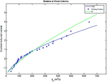
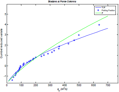
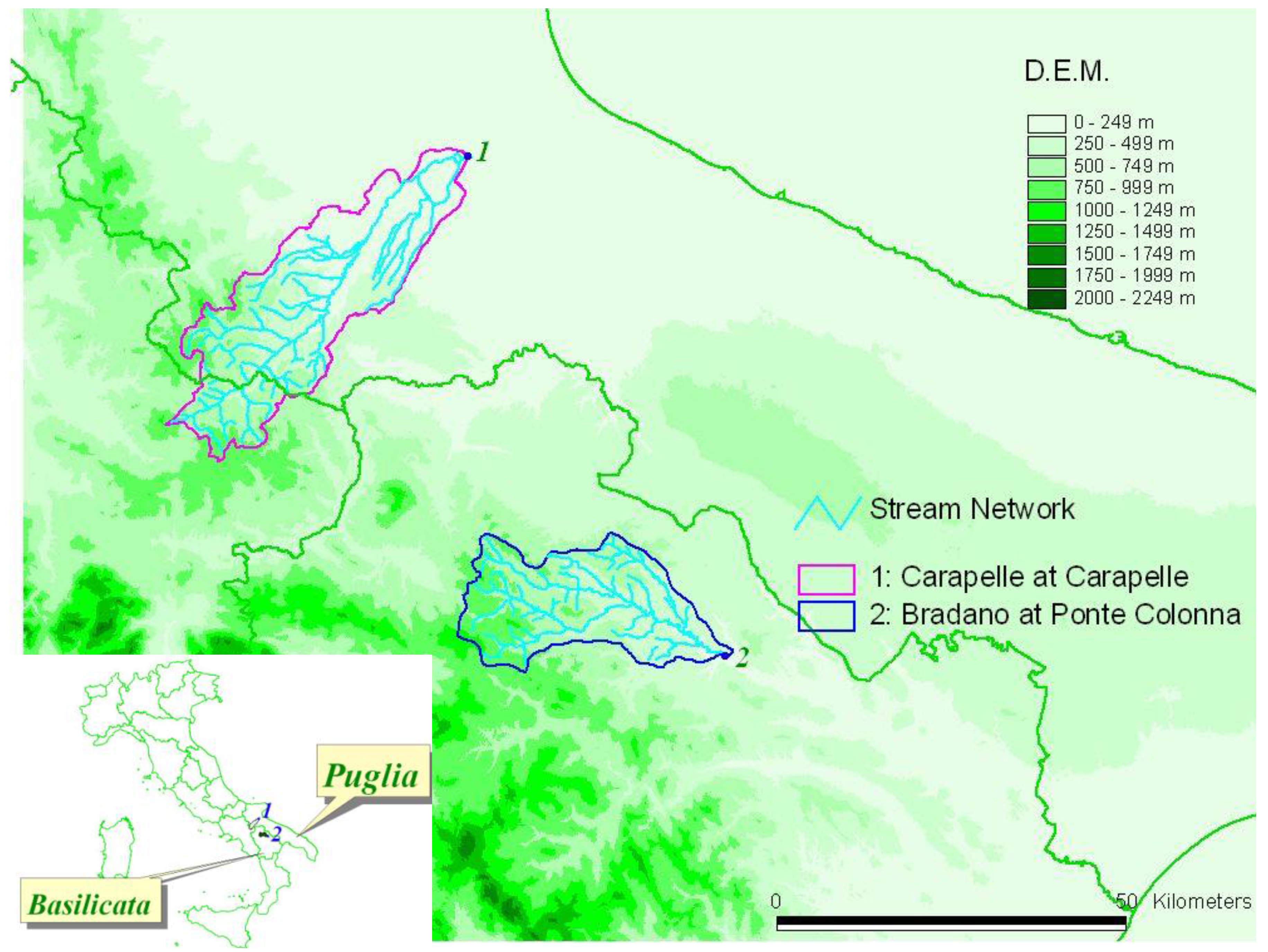
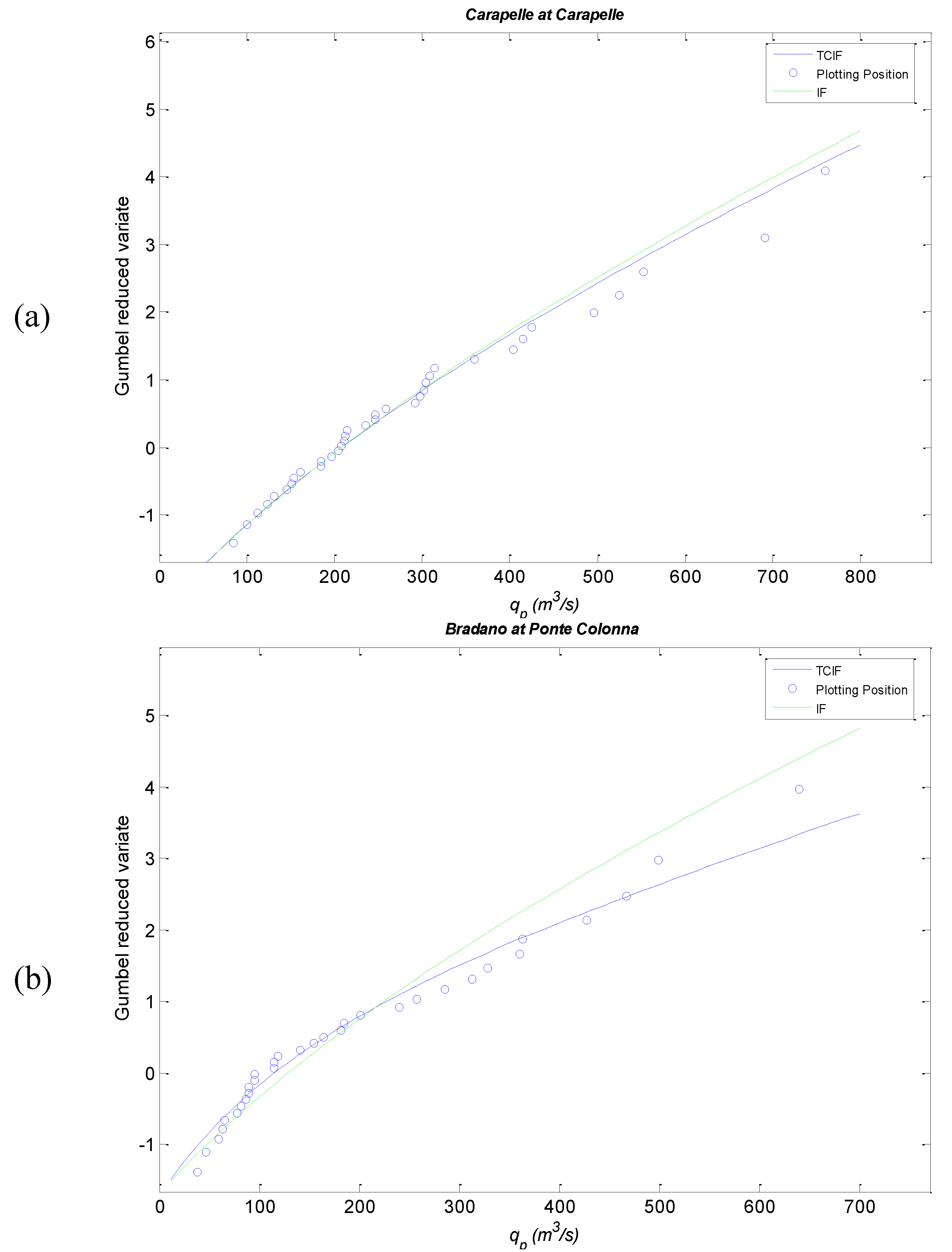
3. Case Studies and Application

In this section, we report results of the application of the IF and TCIF models to two gauged catchments in Southern Italy: the Carapelle river at Carapelle, in Puglia, and the Bradano river at Ponte Colonna, in Basilicata. Puglia and Basilicata are regions in Southern Italy, represented in Figure 1 with the studied basins, their stream network and a 90 m × 90 m digital elevation model (D.E.M.) grid. The main features of the two basins are reported in Table 1, where A is basin area, μ, Cv, Cs and N are, respectively mean, coefficient of variation, coefficient of skewness and sample size of the observed AMFS, I is the Thornthwaite climatic index [38,39], which compares annual precipitation P and annual potential evapotranspiration E_p, I = (P − E_p)/E_p. The climatic index distinguishes, in general, between dry (I < 0) and humid (I > 0) basins. In particular, Carapelle at Carapelle is classified as semi-arid (−0.4 ≤ I < −0.2) and Bradano at Ponte Colonna as dry−subhumid (−0.2 ≤ I < 0). They were selected with the aim of finding the most appropriate model structure for each river basin and, consequently, of detecting the presence of different runoff thresholds affecting the processes responsible for runoff generation.

Figure 1. Basins of Southern Italy selected as case studies.

Figure 1. Basins of Southern Italy selected as case studies.

Table 1. River Basin Characteristics.

	n.	A (km2)	I	(m3/s)	Cv	Cs	N
Carapelle at Carapelle	1	715	-0.23	283.7	057	1.34	36
Bradano at Ponte Colonna	2	462	-0.08	201.6	0.76	1.21	32

Table 1. River Basin Characteristics.

	n.	A (km2)	I	(m3/s)	Cv	Cs	N
Carapelle at Carapelle	1	715	-0.23	283.7	057	1.34	36
Bradano at Ponte Colonna	2	462	-0.08	201.6	0.76	1.21	32

Parameter Estimation and Results

The IF distribution has twelve parameters: baseflow (q_o), four parameters dependent on basin geomorphology (A,τ_A, ξ, β), four rainfall parameters (E[i_A,τ], ε, Λ_p, k), and three parameters (ε^’, Λ_q, r), which are strictly related to runoff generation mechanisms. It is worth mentioning that all parameters, with the exception of r and Λ_q, are not calibrated on the available AMFS. We performed for them a a priori evaluation by using rainfall statistics and other information. Once all the other parameters are known, only two of them (namely r and Λ_q) are estimated by means of the maximum likelihood function evaluated on AMFS.

The TCIF distribution includes the following fifteen parameters: nine of them are already in the IF model (q_o, A, τ_A, ξ, β, E[i_A,τ], ε, Λ_p, k), six more parameters (ε_L, ε _H, Λ_H, Λ_L, r_L, r_H) are strictly related to runoff generation mechanisms. Even in this case, four of them (Λ_H, Λ_L, r_L, r_H,), are obtained from at-site estimation based on the maximum likelihood function evaluated on AMFS, while all remaining parameters are a priori evaluated from information other than AMFS.

We first estimate all parameters of the IF and TCIF distributions which depend on a priori information other than AMFS. Among these, all parameters dependent on precipitation which is analyzed by means of standard regional methods applied to the observed series of annual maxima of rainfall records. Then, the remaining two unknown parameters of the IF model (Λ_q, r) are calibrated using the observed AMFS. Finally, the remaining four unknown parameters of the TCIF model are calibrated by exploiting the IF parameter estimates as initial guess.

Most of the model parameters were estimated in previous studies [17,20,39]. In particular, in Fiorentino and Iacobellis [39], the IF model was applied to several basins in Puglia and Basilicata, including Bradano and Carapelle. Nevertheless we briefly include here the procedures adopted, results are in Table 2. We first describe the evaluation of parameters common to IF and TCIF models. The base flow q_o was estimated as the average monthly flow measured at-site in January and February. There are four parameters dependent on rainfall (E[i_A,τ], ε, Λ_p, k) and they were estimated by means of regional frequency analysis of rainfall annual maximum series (AMS) based on the flood index procedure with hierarchical estimation of parameters [39]: k was dependent on the unique regional coefficient of skewness of rainfall AMS; Λ_p was dependent on the regional estimates of the coefficient of variation (different for Basilicata and Puglia). The expected value of the space-time average rainfall intensity E[i_A,τ] was evaluated exploiting the intensity-duration-frequency (IDF) curve of the expected annual maximum rainfall intensity, obtaining the average of the base process from the annual maxima of a Poisson Process and the US Weather Bureau areal reduction factor [20]. The analysis of the regional scaling of E[i_A,τ], provided the regional estimates of the exponent ε (different for Basilicata and Puglia)

Parameters dependent on basin geomorphology are A,τ_A, ξ, β. Basin area A and lag-time τ_A were available in regional studies of basins in Puglia and Basilicata [39], β = 4 and ξ = 0.7 were assigned as described in the appendix (see also [17] for further details).

The loss threshold scaling factors ε^’, ε_L, ε_H deserve particular attention. For the IF model, ε^’ was equal to 0.5, assuming that in dry basins the prevalent mechanism is of the storage type [39]. On the other hand, the lower and the higher runoff thresholds of the TCIF model are characterized by Equations (8) and (9), respectively, and particularly by the exponents ε_L and ε_H. In particular, Gioia et al. [20] assumed ε_L = 0 and ε_H = 0.5, providing a constant infiltration rate for the lower threshold f_a,L, and a storage behavior for the higher threshold f_a,H.. With this paper being devoted to the analysis of basins in a dry climate, we assumed for both thresholds a capacitive behavior (ε_L = ε_H = 0.5) assuming that a dry state characterizes the antecedent soil moisture conditions of both mechanisms. Such an assumption was confirmed by [40] where the analysis was extended to several other basins of Southern Italy.

Table 2. Estimatedparameter values of the IF and TCIF models.

Site	qo (m3/s)	E[iA,τ] (mm/h)	ε	Λp	k	τA(h)	ξ	β	ε’	Λq
Carapelle at Carapelle	7.0	0.20	0.39	44.6	0.8	9.2	0.7	4	0.5	10.5
Bradano at Ponte Colonna	5.0	0.45	0.33	21.0	0.8	4.3	0.7	4	0.5	5.0
Site	fA (mm/h)	r	εL	ε H	ΛL	ΛH	fA,L (mm/h)	fA,H (mm/h)	rL	rH
Carapelle at Carapelle	1.01	0.45	0.5	0.5	9.86	0.66	1.01	3.86	0.41	0.99
Bradano at Ponte Colonna	2.02	0.30	0.5	0.5	3.98	1.04	2.01	5.08	0.15	0.99

Table 2. Estimatedparameter values of the IF and TCIF models.

Site	qo (m3/s)	E[iA,τ] (mm/h)	ε	Λp	k	τA(h)	ξ	β	ε’	Λq
Carapelle at Carapelle	7.0	0.20	0.39	44.6	0.8	9.2	0.7	4	0.5	10.5
Bradano at Ponte Colonna	5.0	0.45	0.33	21.0	0.8	4.3	0.7	4	0.5	5.0
Site	fA (mm/h)	r	εL	ε H	ΛL	ΛH	fA,L (mm/h)	fA,H (mm/h)	rL	rH
Carapelle at Carapelle	1.01	0.45	0.5	0.5	9.86	0.66	1.01	3.86	0.41	0.99
Bradano at Ponte Colonna	2.02	0.30	0.5	0.5	3.98	1.04	2.01	5.08	0.15	0.99

For the remaining parameters of the IF model, we derived from Equation (6) the relationship

$$f_A={\left[{E[i}_{\text{A,τ}}^k]\hspace{0.17em}\log \left(\frac{{\Lambda }_p}{{\Lambda }_q}\right)\right]}^{\raisebox{1ex}{$1$}\!\left/ \!\raisebox{-1ex}{$k$}\right.}$$

(15)

providing f_A as a function of Λ_q, once the a priori estimates of k, Λ_p, E[i_A,τ] are available, and we carried out an at-site evaluation procedure of parameters Λ_q and r based on minimizing a negative log likelihood function evaluated on AMFS. The procedure was performed by exploring the domain of feasible parameter values on a regular grid. In particular, the grid-dataset values was prepared with r ranging from 0.01 to 1, with step 0.01, and Λ_q from 0.1 to Λ_p, with step 0.1. For each test basin, the best parameters dataset was chosen as the one minimizing a negative log likelihood function of the observed sample of annual maximum floods.

Analogously, for the remainder parameters of the TCIF model, we used Equations (12) in order to obtain the expression of f_A,L and f_A,H, using the a priori estimates of k, Λ_p, E[i_A,τ]:

$$f_{A,L}={\left[{E[i}_{A,\tau }^k]\hspace{0.17em}\log \left(\frac{{\Lambda }_p}{{\Lambda }_L+{\Lambda }_H}\right)\right]}^{\raisebox{1ex}{$1$}\!\left/ \!\raisebox{-1ex}{$k$}\right.}\hspace{0.17em}\text{and}\hspace{0.17em}{f}_{A,H}={\left[{E[i}_{A,\tau }^k]\hspace{0.17em}\hspace{0.17em}\text{log}\left(\frac{{\Lambda }_p}{{\Lambda }_H}\right)\right]}^{\raisebox{1ex}{$1$}\!\left/ \!\raisebox{-1ex}{$k$}\right.}$$

(16)

then, parameters Λ_L,Λ_H, r_L, r_H were calibrated adopting a maximum likelihood procedure.

In this case, in order to avoid the cumbersome exploration of the entire parameters domain on a regular grid, we used as initial guess values r = r_L = r_H, Λ_H = 0 and Λ_L = Λ_q. These values correspond to the hypothesis that TCIF distribution collapses into IF distribution. Starting from the initial guess values, the maximum likelihood was found exploring the four-dimensional space of parameters r_L, r_H, Λ_H, Λ_L by following the direction of maximum slope of the negative log-likelihood function. In particular, consistently with definitions of the L-type and H-type events we assumed that r_L may only decrease from r to 0, while r_H ranges from r to 1, both with step 0.01; also Λ_L ranges from Λ_q to Λ_p and Λ_H varies, accordingly (i.e., always respecting the condition Λ_L + Λ_H ≤ Λ_p) from 0 to Λ_p. The selected parameter-datasets are reported in Table 2, where it is worth noting that the lower threshold f_a,L of the TCIF model corresponds to the single threshold of the IF model. Slight differences are found with respect to the estimates of r and f_A reported in Fiorentino and Iacobellis [39], which used regional estimates of Λ_q for evaluating f_A, and only r was calibrated by equating an approximate expression of the IF first order moment to the observed mean annual flood.

In Figure 2 we display the TCIF-CDF, the IF-CDF and the Weibull plotting positions of the AMFS of test basins in a Gumbel probability plot. From the visual comparison, one may note the difference between the two distributions which is slight for the semi-arid Carapelle basin while it is more pronounced in the case of the dry-subhumid Bradano basin, the latter being characterized by a more skewed distribution (e.g., [41,42]). In order to objectively assess the “right” model for each test basin, we investigated, as reported in next section, the use of statistical techniques for the “best” model selection.

Figure 2. Comparison between TCIF and IF CDFs and the Weibull plotting positions of the annual maximum flood series: (a) Carapelle at Carapelle and (b) Bradano at Ponte Colonna.

Figure 2. Comparison between TCIF and IF CDFs and the Weibull plotting positions of the annual maximum flood series: (a) Carapelle at Carapelle and (b) Bradano at Ponte Colonna.

4. Model Selection Procedure

The selection of the best statistical model, for a given sample series, is often based on inference tests depending, for example, on the significance level chosen. In statistical hydrology they are often used in the particular case of nested distributions (e.g., the Gumbel, Frechet and GEV distributions). With the increase of computer capabilities many methods have been proposed and developed for model selection on cross-validation techniques, also in fields other than hydrology (e.g., [43,44]). In this work, five different methods for model selection criteria are used with the aim of finding the most appropriate model structure between the IF and TCIF models.

In particular, we first considered the log-likelihood criterion (LLC), which does not use any penalty term, the Akaike information criterion (AIC) proposed by Akaike [45], who introduced the principle of maximum entropy for model selection, and the Bayesian information criterion (BIC) proposed by Schwarz [46]. Both AIC and BIC adopt a penalty term accounting for the number of model parameters. The fourth method is the log-likelihood ratio test (LLR). Finally, the generalization criterion proposed by Busemeyer and Wang [36]. Mosier [43] was the first to present a clear definition of the cross-validation criterion. Others have shown that the cross-validation criterion is asymptotically equivalent to the AIC [47,48]. Nevertheless, the generalization criterion is based on a priori predictions made before observing the data. Thus it objectively assesses the model capability to predict states different from those observed and used for model calibration.

The LLC for the jth operational model is simply evaluated as:

$${\text{LLC}}_j=-2\hspace{0.17em}\ln [{\mathrm{L}}_j({\vartheta }_j,x)]$$

(17)

where $L_j({\vartheta }_j,x)={\displaystyle \prod _{i=1}^n{g}_j}(x_i,{\vartheta }_j)$ is the likelihood function, evaluated at the point ϑ = ϑ_j, corresponding to the maximum likelihood estimator of the parameter vector ϑ [49].

The AIC for the jth operational model may be computed as:

$${AIC}_j=-2\hspace{0.17em}\ln [L_j({\vartheta }_j,\mathrm{x})]+2p_j$$

(18)

where $L_j({\vartheta }_j,x)={\displaystyle \prod _{i=1}^n{g}_j}(x_i,{\vartheta }_j)$ is the likelihood function, evaluated at the point ϑ = ϑ_j, corresponding to the maximum likelihood estimator of the parameter vector ϑ [49], and p_j is the number of estimated parameters of the j_th operational model. By analyzing Equation (18), one can see that the first term on the right-hand side tends to decrease as more parameters are added to the approximating model, while the second term tends to increase. Note that the penalty term tends to select simpler models under the principle of parsimony. Sugiura [50] derived a second-order variant of AIC, called AICc, valid in the case of a small sample size n, with respect to the number of estimated parameters p (n/p < 40):

$${AICc}_j=-2\hspace{0.17em}\ln [L_j({\vartheta }_j,\mathrm{x})]+2p_j\left(\frac{\text{n}}{\text{n}-p_j-1}\right)$$

(19)

BIC for the j_th operational model is evaluated as follows:

$${BIC}_j=-2\hspace{0.17em}\ln [L_j({\vartheta }_j,\mathrm{x})]+\ln (n){\mathrm{p}}_{\mathrm{j}}$$

(20)

In practical application one selects the model with the minimum value of the discrepancy measure LLC, AIC or BIC.

Table 3 shows the results of these three selection criteria applied to IF and TCIF. The two criteria (AICc and BIC) accounting for model parsimony suggests rejection of the hypothesis that the AFMS of the two river basins investigated are extracted from the TCIF model which has more parameters, while the negative log-likelihood selection criteria chooses, always, the TCIF model.

Table 3. Application of model selection techniques.

Site	LLC		AICc		BIC		LLR
	IF	TCIF	IF	TCIF	IF	TCIF	( IF, TCIF )
Carapelle at Carapelle	453.12	452.94	457.48	462.23	460.28	467.27	0.18
Bradano at Ponte Colonna	397.29	395.66	401.71	405.14	404.23	409.52	1.63

Table 3. Application of model selection techniques.

Site	LLC		AICc		BIC		LLR
	IF	TCIF	IF	TCIF	IF	TCIF	( IF, TCIF )
Carapelle at Carapelle	453.12	452.94	457.48	462.23	460.28	467.27	0.18
Bradano at Ponte Colonna	397.29	395.66	401.71	405.14	404.23	409.52	1.63

The log-likelihood ratio test, which is specifically suited for comparisons among nested models, introduces the log-likelihood ratio statistic for two different models i and j:

$$\text{LLR}\left(i,j\right)=-2\hspace{0.17em}\ln [{\mathrm{L}}_i({\vartheta }_i,x)/{\mathrm{L}}_{\mathrm{j}}({\vartheta }_j,x)]={\text{LLC}}_i-{\text{LLC}}_j$$

whose probability distribution can be approximated by a chi-square (χ²) distribution with (p_i − p_j) degrees of freedom. In this test, if LLR(i,j), where model i is nested within model j, exceeds a cutoff (${\chi }_{\ast }^2$), which depends on the test significance level, then the null hypothesis that implies no significant model differences (H₀), is rejected. The results in Table 3 show that even the log-likelihood ratio test, which accounts for model parsimony by mean of the chi-square degrees of freedom, always select the IF distribution as being the LLR values well below the cutoff value ${\chi }_{\ast }^2$ = 5.99 obtained for significance level α = 0.05 and degrees of freedom = 2.

These results pose a serious question which, for the case of theoretically derived distributions, also has implications on the individuation of the main processes that affect runoff generation. Is it suitable, in this case, to recourse to such selection criteria accounting for model parsimony? An objective answer was found by introducing the generalization criterion which is based on a priori predictions made by mean of a split-sample procedure. More precisely, the procedure is structured as follows: (1) For each river basin, the sample of AMFS is divided into two sub-samples statistically independent of sizes N₁ and N₂ (where the total number N = N₁ + N₂). (2) During the first calibration stage, best fitting parameter estimates ϑ_IF and ϑ_TCIF are obtained from the sub-sample N₁, respectively by selecting parameters of the IF and the TCIF models that minimize the discrepancy (D) evaluated as negative log-likelihood function (${\mathrm{D}}_{\mathrm{I}\mathrm{F},{\mathrm{N}}_1}=-2\hspace{0.17em}\ln [L({\vartheta }_{\mathrm{I}\mathrm{F}},{\mathrm{N}}_1)]$ and ${\mathrm{D}}_{\mathrm{T}\mathrm{C}\mathrm{I}\mathrm{F},N_1}=-2\hspace{0.17em}\ln [L({\vartheta }_{\mathrm{T}\mathrm{C}\mathrm{I}\mathrm{F}},{\mathrm{N}}_1)]$) applied to the observed sub-sample N₁. (3) During the second validation stage the previously estimated parameters, ϑ_IF and ϑ_TCIF, are exploited to compare the two models in terms of their predictive performance calculating the negative log-likelihood function (D_IF,N2 and D_TCIF,N2) with respect to the second independent sample N₂. (4) The difference between the predictive performance of the two models (δ_p = D_TCIF,N2 − D_IF,N2) is calculated. (5) Steps 1–4 are repeated 100 times by randomly selecting different sub-samples to produce mean and standard deviation (μ(δ_p) and σ(δ_p)) of the δ_p factor. If μ(δ_p) > 0 the IF model is selected and, otherwise, TCIF. The application of this criterion to test basins selected the TCIF model as a better model for both as reported in Table 4 where μ(δ_p) and σ(δ_p) are shown.

These results suggest that when cross-validation techniques cannot be applied due to small sample size, the log-likelihood criterion, without any penalty factor accounting for model parsimony, should be preferred when dealing with such nested distributions.

Table 4. Application of generalization criterion for model selection.

Carapelle at Carapelle				Bradano at Ponte Colonna
N1	N2	μ(δp)	σ(δp)	N1	N2	μ(δp)	σ(δp)
18	18	−0.17	−4.04	16	16	−0.89	−1.61

Table 4. Application of generalization criterion for model selection.

Carapelle at Carapelle				Bradano at Ponte Colonna
N1	N2	μ(δp)	σ(δp)	N1	N2	μ(δp)	σ(δp)
18	18	−0.17	−4.04	16	16	−0.89	−1.61

5. Conclusions

An improvement in flood prediction is expected by selecting the most appropriate model scheme for representing real processes and, consequently, for detecting dominant mechanisms responsible for non-linearity in flood distributions. A comparison between the IF and TCIF models was made using data from two river basins in semi-arid and dry-subhumid climate.

The TCIF model, which generalizes the IF model, introduces two different threshold mechanisms as responsible for ordinary and extraordinary events, in analogy with the theory of the TCEV distribution [26]: The first one is characterized by frequent occurrences and lower average of exceedances (L-type), the second one includes rare events and higher average of exceedances (H-type).

Results of this work show that two different mechanisms of runoff generation may be observed in dry-subhumid and semi-arid climates. In fact, while it is already recognized in the international hydrologic literature that non linear effects in flood frequency distribution may depend on the alternation of infiltration and saturation excess (e.g., [22]), it is less common to observe those different runoff mechanisms in dry climate.

We have shown that a high-frequency behavior may be provided by a storage threshold affecting smaller areas of the basin while the low-frequency component may arise when a higher storage threshold is exceeded in large areas of a basin. Such important results are also compatible with the occurrence of a saturation excess process at the lower component being sometimes modeled as a storage process too (e.g., [22,29]).

We introduced a novel and faster procedure for the estimation of parameters of the TCIF distribution. This is based on the individuation of the maximum-likelihood parameter dataset and is linked to the estimated parameters of the IF distribution, which are used as initial guess while the exploration of the likelihood function is performed respecting the physical constrains r_L ≤ r, r_H ≥ −r and Λ_L + Λ_H ≤ Λ_p on the domain of parameter values. Such a procedure is of general interest and may be applied at any climate in any basin were floods are typically rainfall-driven.

Finally, interesting results were obtained in the framework of model selection, in the case of nested distributions IF and TCIF. The comparison was made through the use of selection criteria able to account for the more appropriate model structure. We observed that the selection criteria based on the log-likelihood function, without penalty term, tends to prefer the TCIF model even in the Carapelle basin that does not display a high non-linearity. On the other hand, criteria accounting for a penalty factor related to the number of parameters, such as the AIC, the BIC and the chi-square test, systematically select the IF distribution. This happens also for the dry-subhumid Bradano basin, notwithstanding the TCIF distribution provides a clear better fit to the right tail of the observed distribution (see Figure 2). Then, we referred to the generalized criterion based on a split-sample procedure that objectively tests the a priori predictive capability of the model. In both test basins the generalized criterion selected the TCIF distribution, thus providing significant support for its structural validity and further reinforcing its conceptual representation of the hydrologic processes dominant at basin scale. Such results confirm what was already stated by Busemeyer and Wang [36]: both the Akaike (AIC) information criterion and the Bayesian information criterion (BIC), as well as other methods including a penalty factor, should not be considered appropriate for selecting between nested distributions. They also observed that “it is well known that the chi-square criterion tends to pick the oversimplified model, with small sample sizes that suffer from a lack of statistical power, and it tends to pick the overly complex model in large sample sizes that enjoy extremely high statistical power”. Only the generalized criterion, which is based on cross-validation, performs a priori predictions and provides an objective assessment of the model predictive ability. Obviously, the generalized criterion is applicable only to AMFS with minimum length of 30 years, with sub-samples of 15 years used for calibration and validation. Thus, the use of a log-likelihood criterion, without any penalty factor accounting for model parsimony, is recommended when dealing with nested distributions and small sample size. Further investigation on techniques for model selection with diagnostic ability (i.e., able to evaluate model structure validity) is the object of ongoing research and future developments by the authors.

References and Notes

1. Sivapalan, M.; Takeuchi, K.; Franks, S.W.; Gupta, V.K.; Karambiri, H.; Lakshmi, V.; Liang, X.; McDonnell, J.J.; Mendiondo, E.M.; O’Connell, P.E.; Oki, T.; Pomeroy, J.W.; Schertzer, D.; Uhlenbrook, S.; Zehe, E. IAHS Decade on Predictions in Ungauged Basins (PUB), 2003–2012: Shaping an exciting future for the hydrological sciences. Hydrol. Sci. J. 2003, 48, 857–880. [Google Scholar]
2. Abdulla, F.A.; Lettenmaier, D.P. Development of regional parameter estimation equations for a macro scale hydrologic model. J. Hydrol. 1997, 197, 30–57. [Google Scholar]
3. Seibert, J. Regionalisation of parameters of a conceptual rainfall-runoff model. Agric. For. Meteorol. 1999, 98-99, 279–293. [Google Scholar]
4. Fernandez, W.; Vogel, R.M.; Sankarasubramanian, A. Regional calibration of a watershed model. Hydrol. Sci. J. 2000, 45, 689–707. [Google Scholar] [CrossRef]
5. Hundecha, Y.; Bardossy, A. Modeling of the effect of land use changes on the runoff generation of a river basin through parameter regionalization of a watershed model. J. Hydrol. 2004, 292, 281–295. [Google Scholar] [CrossRef]
6. Merz, B.; Blöschl, G. Regionalisation of watershed model parameters. J. Hydrol. 2004, 287, 95–123. [Google Scholar] [CrossRef]
7. Wagener, T.; Wheater, H.S. Parameter estimation and regionalization for continuous rainfall-runoff models including uncertainty. J. Hydrol. 2006, 320, 132–154. [Google Scholar] [CrossRef]
8. Heuvelmans, G.; Muys, B.; Feyen, J. Regionalisation of the parameters of a hydrological model: Comparison of linear regression models with artificial neural nets. J. Hydrol. 2006, 319, 245–265. [Google Scholar] [CrossRef]
9. Post, D.A.; Jakeman, A.J. Predicting the daily streamflow of ungauged watersheds in S.E. Australia by regionalizing the parameters of a lumped conceptual rainfall-runoff model. Ecol. Model. 1999, 123, 91–104. [Google Scholar]
10. Wagener, T.; Wheater, H.S.; Gupta, H.V. Rainfall-runoff Modelling in Gauged and Ungauged Catchments; Imperial College Press: London, UK, 2004; p. 300. [Google Scholar]
11. Wagener, T.; Sivapalan, M.; McDonnell, J.J.; Hooper, R.; Lakshmi, V.; Liang, X.; Kumar, P. Predictions in ungauged basins (PUB)—A catalyst for multi-disciplinary hydrology. Eos. Trans. AGU 2004, 85, 451–452. [Google Scholar] [CrossRef]
12. McIntyre, N.; Lee, H.; Wheater, H.S.; Young, A.; Wagener, T. Ensemble predictions of runoff in ungauged catchments. Water Resour. Res. 2005, 41, W12434. [Google Scholar]
13. Young, A.R. Stream flow simulation within UK ungauged watersheds using a daily rainfall-runoff model. J. Hydrol. 2006, 320, 155–172. [Google Scholar]
14. McDonnell, J.J.; Woods, R. On the need for catchment classification. J. Hydrol. 2004, 299, 2–3. [Google Scholar] [CrossRef]
15. Eagleson, P. Dynamics of flood frequency. Water Resour. Res. 1972, 8, 878–898. [Google Scholar] [CrossRef]
16. Gottschalk, L.; Weingartner, R. Distribution of peak flow derived from a distribution of rainfall volume and runoff coefficient, and a unit hydrograph. J. Hydrol. 1998, 208, 148–162. [Google Scholar] [CrossRef]
17. Iacobellis, V.; Fiorentino, M. Derived distribution of floods based on the concept of partial area coverage with a climatic appeal. Water Resour. Res. 2000, 36, 469–482. [Google Scholar] [CrossRef]
18. De Michele, C.; Salvadori, G. On the derived flood frequency distribution: Analytical formulation and the influence of antecedent soil moisture condition. J. Hydrol. 2002, 262, 245–258. [Google Scholar] [CrossRef]
19. Franchini, M.; Galeati, G.; Lolli, M. Analytical derivation of the flood frequency curve through partial duration series analysis and a probabilistic representation of the runoff coefficient. J. Hydrol. 2005, 303, 1–15. [Google Scholar] [CrossRef]
20. Gioia, A.; Iacobellis, V.; Manfreda, S.; Fiorentino, M. Runoff thresholds in derived flood frequency distributions. Hydrol. Earth Syst. Sci. 2008, 12, 1295–1307. [Google Scholar]
21. Strupczewski, W.G.; Singh, V.P.; Weglarczyk, S. Physics of Environmental Frequency Analysis. In Integrated Technologies for Environmental Monitoring and Information Production; Harmancioglu, N.B., Ozkul, S.D., Fistikoglu, O., Geerders, P., Eds.; Kluwer Academic Publishers: Dordrecht, The Netherlands, 2003; NATO Science Series: IV: Earth and Environmental Sciences; Vol. 23, pp. 195–172. [Google Scholar]
22. Sivapalan, M.; Wood, E.F.; Beven, K.J. On hydrologic similarity, 3. A dimensionless flood frequency model using a generalized geomorphologic unit hydrograph and partial area runoff generation. Water Resour. Res. 1990, 26, 43–58. [Google Scholar]
23. Vander Kwaak, J.E.; Loague, K. Hydrologic-response simulations for the R-5 catchment with a comprehensive physics-based model. Water Resour. Res. 2001, 37, 999–1013. [Google Scholar] [CrossRef]
24. Allamano, P.; Claps, P.; Laio, F. An analytical model of the effects of catchment elevation on the flood frequency distribution. Water Resour. Res. 2009, 45, W01402. [Google Scholar] [CrossRef]
25. Waylen, P.; Woo, M. Prediction of annual floods generated by mixed processes. Water Resour. Res. 1982, 18, 1283–1286. [Google Scholar] [CrossRef]
26. Rossi, F.; Fiorentino, M.; Versace, P. Two-component extreme value distribution for flood frequency analysis. Water Resour. Res. 1984, 20, 847–856. [Google Scholar] [CrossRef]
27. Buishand, T.; Demaré, G. Estimation of the annual maximum distribution from samples of maxima in separate seasons. Stochastic Hydrol. Hydraul. 1990, 4, 89–103. [Google Scholar] [CrossRef]
28. Alila, Y.; Mtiraoui, A. Implications of heterogeneous flood-frequency distributions on traditional stream-discharge prediction techniques. Hydrol. Proc. 2002, 16, 1065–1084. [Google Scholar] [CrossRef]
29. Sivapalan, M.; Blöschl, G.; Merz, R.; Gutknecht, D. Linking flood frequency to long-term water balance: Incorporating effects of seasonality. Water Resour. Res. 2005, 41, W06012. [Google Scholar]
30. Rahman, A.; Weinmann, P.; Hoang, T.; Laurenson, E. Monte Carlo simulation of flood frequency curves from rainfall. J. Hydrol. 2002, 256, 196–210. [Google Scholar] [CrossRef]
31. Blazkova, S.; Beven, K. Flood frequency estimation by continuous simulation of subcatchment rainfalls and discharges with the aim of improving dam safety assessment in a large basin in the Czech Republic. J. Hydrol. 2004, 292, 153–172. [Google Scholar] [CrossRef]
32. Fiorentino, M.; Manfreda, S.; Iacobellis, V. Peak runoff contributing area as hydrological signature of the probability distribution of floods. Adv. Water Resour. 2007, 30, 2123–2134. [Google Scholar] [CrossRef]
33. Beven, K.J. Rainfall-Runoff Modeling—The Primer; Wiley: Chichester, UK, 2001. [Google Scholar]
34. Wagener, T.; Gupta, H.V. Model identification for hydrological forecasting under uncertainty. Stoch. Environ. Res. Risk Assess. 2005, 19, 378–387. [Google Scholar] [CrossRef]
35. Laio, F.; Di Baldassarre, G.; Montanari, A. Model selection techniques for the frequency analysis of hydrological extremes. Water Resour. Res. 2009, 45, W07416. [Google Scholar] [CrossRef]
36. Busemeyer, J.R.; Wang, Y.M. Model comparisons and model selections based on generalization criterion methodology. J. Math. Psychol. 2000, 44, 171–189. [Google Scholar] [CrossRef] [PubMed]
37. Kottegoda, N.T.; Rosso, R. Statistics, Probability and Reliability for Civil and Environmental Engineers; McGraw-Hill: New York, NY, USA, 1997. [Google Scholar]
38. Thornthwaite, C.W. An approach toward a rational classification of climate. Am. Geograph. Rev. 1948, 38, 55–94. [Google Scholar] [CrossRef]
39. Fiorentino, M.; Iacobellis, V. New insights about the climatic and geologic control on the probability distribution of floods. Water Resour. Res. 2001, 37, 721–730. [Google Scholar] [CrossRef]
40. Fiorentino, M.; Gioia, A.; Iacobellis, V.; Manfreda, S. Regional analysis of runoff thresholds behaviour in Southern Italy based on theoretically derived distributions. Adv. Geosci. 2010, (in press). [Google Scholar]
41. Matalas, N.C.; Slack, J.R.; Wallis, J.R. Regional skew in search of a parent. Water Resour. Res. 1975, 11, 815–826. [Google Scholar] [CrossRef]
42. Cunnane, C. Review of statistical models for flood frequency estimation. In Proceedings of the International Symposium on Flood Frequency and Risk Analysis, Louisiana State University, Baton Rouge, LA, USA, 14–17 May 1986.
43. Mosier, C.I. Problems and designs of cross-validation. Educ. Psychol. Meas. 1951, 11, 5–11. [Google Scholar] [CrossRef]
44. Camstra, A.; Boomsma, A. Cross-validation in regression and covariance structure analysis: An overview. Sociol. Method. Res. 1992, 21, 89–115. [Google Scholar] [CrossRef]
45. Akaike, H. Information theory and an extension of the maximum likelihood principle. In Proceedings of the Second International Symposium on Information Theory, Tsahkadsor, Armenia, 2–8 September 1971; Petrov, B.N., Csaki, F., Eds.; Akademiai Kiado: Budapest, Hungary, 1973; pp. 267–281. [Google Scholar]
46. Schwarz, G. Estimating the dimension of a model. Ann. Stat. 1978, 6, 461–464. [Google Scholar] [CrossRef]
47. Stone, M. On asymptotic equivalence of choice of model by cross-validation and Akaike’s criterion. J. Roy. Stat. Soc. Ser. B 1977, 39, 44–47. [Google Scholar]
48. Browne, M.; Cudeck, W. Single Sample cross-validation indices for covariance structures. Multivariate Behav. Res. 1989, 24, 445–455. [Google Scholar]
49. Linhart, H.; Zucchini, W. Model Selection; John Wiley: Hoboken, NJ, USA, 1986. [Google Scholar]
50. Sugiura, N. Further analysis of the data by Akaike’s information criterion and the finite corrections. Commun. Stat. Theory Methods 1978, A7, 13–26. [Google Scholar] [CrossRef]