Mapping Irrigated Areas Using MODIS 250 Meter Time-Series Data: A Study on Krishna River Basin (India)

Abstract
:1. Introduction
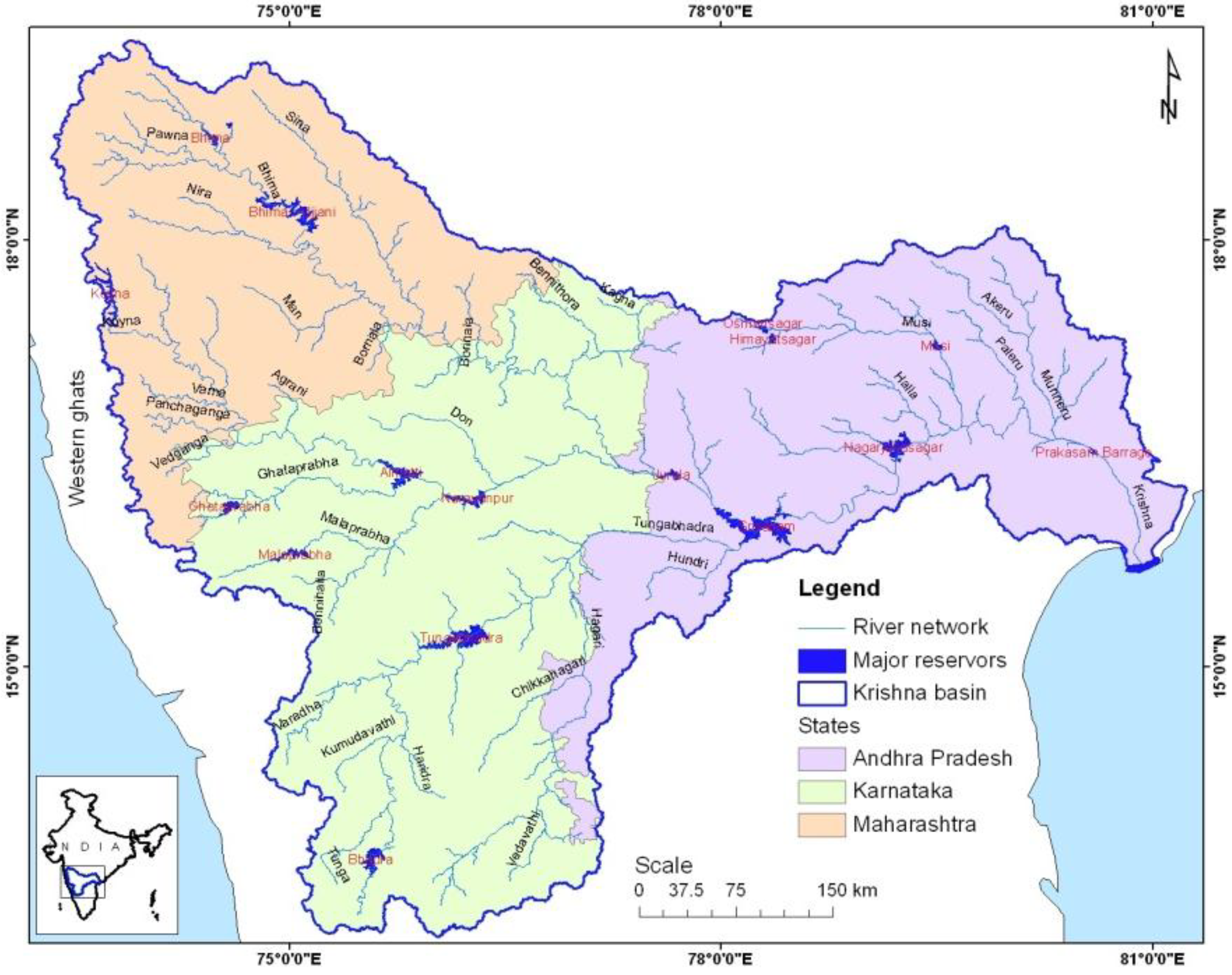
2. Study Area
3. Data
3.1. MODIS Time Series Data

| MOD09A1 product ¹ | |||
| MODIS Bands ² | Band width (nm ³) | Band center (nm ³) | potential application 4 |
| 1 | 620–670 | 648 | Absolute Land Cover Transformation, Vegetation Chlorophyll |
| 2 | 841–876 | 858 | Cloud Amount, Vegetation Land Cover Transformation |
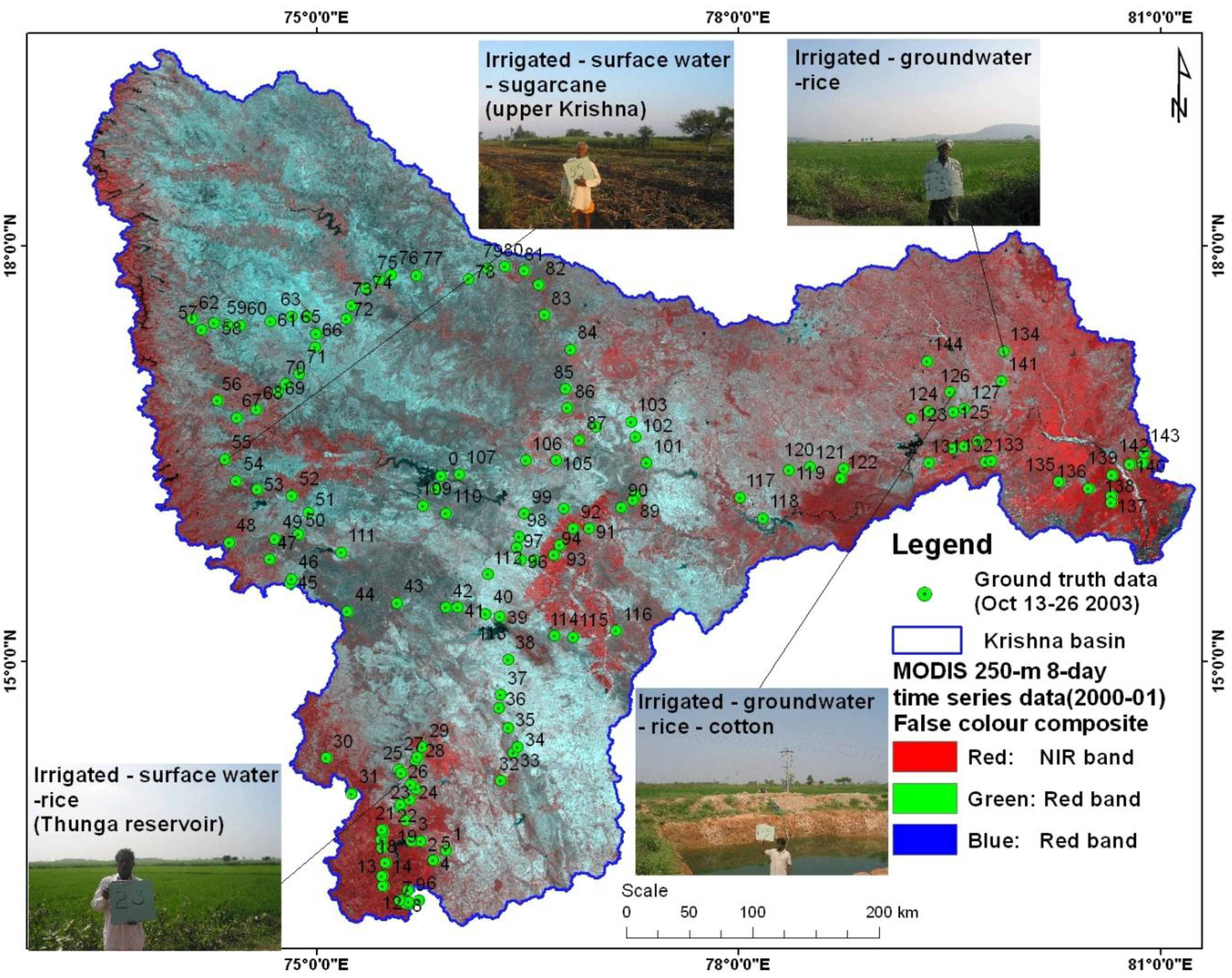
3.2. Groundtruth Datasets
4. Methods
4.1. MODIS NDVI Time-Series Classification
4.2. Class Signatures and NDVI-Reflectivity Thresholds

4.3. Class Lebeling and Sub-Pixel Area Calculations
4.4. Irrigated Fractions
| Full pixel area | Vegetation cover percent (mean) | Irrigation fraction percent | |||||||||
| Tree | Shrubs | Grass | Others | Open | Crop | SW | GW | ||||
| Class1: Water bodies | 517,782 | - | - | - | - | - | - | - | - | - | |
| Class2: Shrublands mix with rangelands | 6,521,637 | 15 | 6.7 | 24.3 | 6.9 | 14.2 | 8.6 | 39.3 | - | - | Grains, oilseeds |
| Class3: Rangelands mix with rainfed | 1,044,788 | 33 | 0.7 | 1.0 | 22.0 | 19.1 | 15.1 | 42.2 | - | - | Grains, oilseeds, pulses |
| Class4: Rainfed agriculture | 5,910,620 | 17 | 4.8 | 5.0 | 9.9 | 8.7 | 4.9 | 66.8 | - | - | Rice, grains, oilseeds, pulses |
| Class5: Rainfed + groundwater | 3,013,915 | 25 | 2.1 | 1.3 | 3.4 | 7.1 | 10.6 | 75.6 | 5.8 | 94.2 | Rice, oilseeds, pulses, grains, cotton, chili |
| Class6: Minor irrigated (light/tank) | 2,122,196 | 6 | 1.5 | 1.1 | 2.9 | 6.3 | 3.7 | 84.5 | 82.3 | 17.7 | Cotton, grains, oilseeds, rice |
| Class7: Irrigated-sw + gw-continuous crops | 2,720,606 | 10 | 2.7 | 2.0 | 1.7 | 2.3 | 2.4 | 88.9 | 31.5 | 68.5 | Sugarcane, rice, chilli, cotton |
| Class8: Irrigated-sw-double crop | 2,487,827 | 22 | 1.7 | 3.7 | 1.9 | 2.8 | 2.2 | 87.6 | 89.5 | 10.5 | Rice, grains, pulses |
| Class9: Forests | 2,235,830 | 12 | 60.2 | 11.2 | 3.0 | 2.7 | 1.6 | 21.3 | - | - | Teak, coffee, aracanut, rice |
| Basin total | 26,575,200 | 140 | 10.0 | 6.2 | 6.5 | 7.9 | 6.1 | 63.3 | |||
5. Results and Discussions
5.1. LULC Fractions
= 2,487,827 × (87.6/100) = 2,180,318 ha
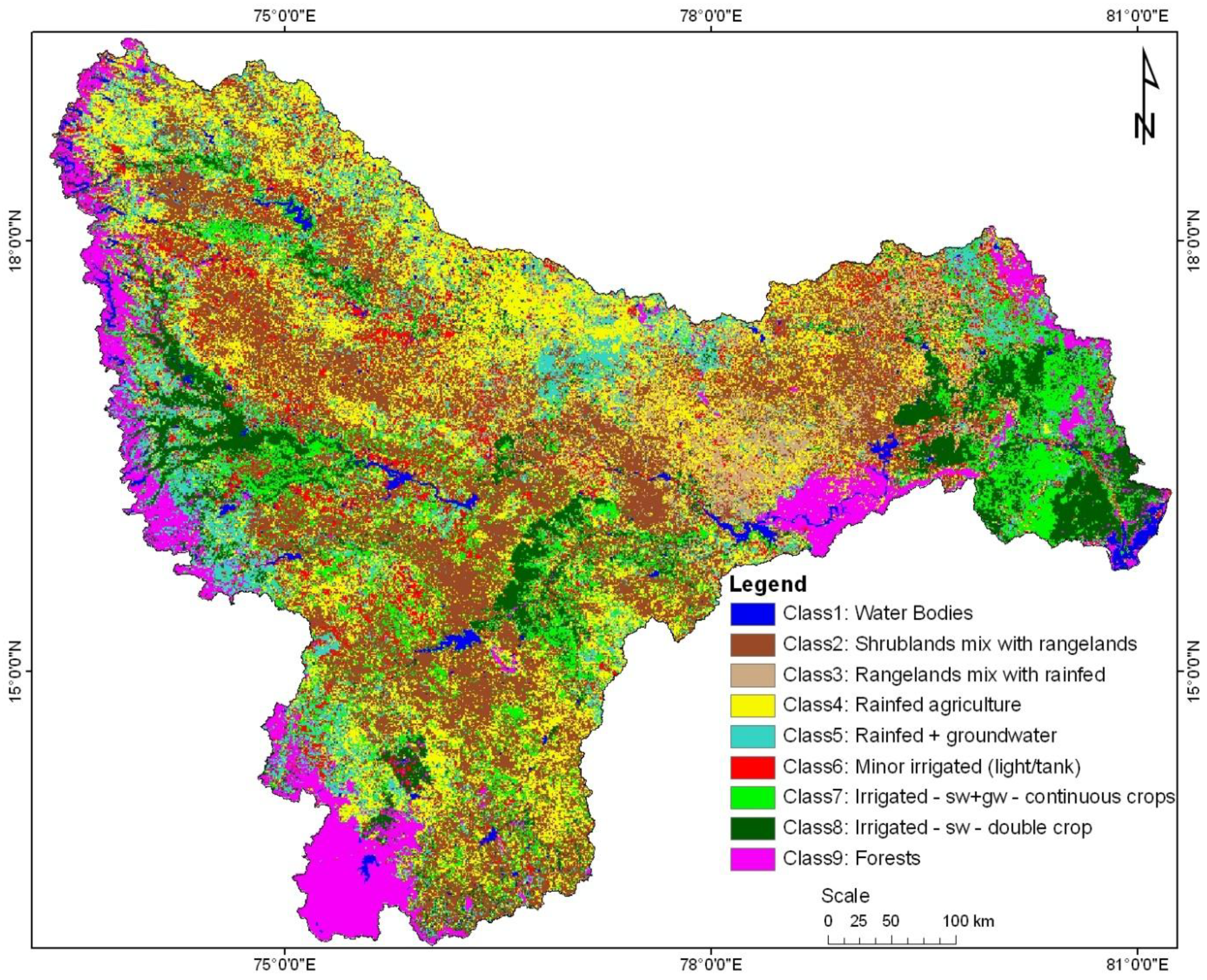
5.2. Land Use Land Cover Maps and Area Statistics
| LULC | % | Land use/ land cover area with in the classes (ha) | Basin totals | |||||
| water | Tree | Shrubs | Grass | Others | Crop | |||
| Class1: Water bodies | 1.9 | 517,782 | - | - | - | - | - | 517,782 |
| Class2: Shrublands mix with rangelands | 24.5 | - | 437,083 | 1,585,240 | 448,825 | 1,487,385 | 2,563,104 | 6,521,637 |
| Class3: Rangelands mix with rainfed | 3.9 | - | 6,962 | 10,443 | 229,753 | 357,162 | 440,467 | 1,044,788 |
| Class4: Rainfed agriculture | 22.2 | - | 282,660 | 293,304 | 583,059 | 801,460 | 3,950,137 | 5,910,620 |
| Class5: Rainfed + groundwater | 11.3 | - | 62,623 | 38,850 | 102,053 | 531,505 | 2,278,884 | 3,013,915 |
| Class6: Minor irrigated (light/tank) | 8.0 | - | 32,783 | 23,141 | 61,709 | 212,123 | 1,792,441 | 2,122,196 |
| Class7: Irrigated,conjunctive | 10.2 | - | 74,024 | 54,763 | 45,321 | 128,259 | 2,418,239 | 2,720,606 |
| Class8: Irrigated, surface water, double crop | 9.4 | - | 42,312 | 92,091 | 47,290 | 125,816 | 2,180,318 | 2,487,827 |
| Class9: Forests | 8.4 | - | 1,346,418 | 249,751 | 67,097 | 95,427 | 477,136 | 2,235,830 |
| Basin totals | 100.0 | 517,782 | 2,284,865 | 2,347,582 | 1,585,107 | 3,739,138 | 16,100,726 | 26,575,200 |
| Total Surface Irrigated area (ha) | 16.3 | 4,319,928 | ||||||
| Total Groundwater Irrigated area (ha) | 16.4 | 4,349,953 | ||||||
| Totaol Irrigated areas (ha) | 32.6 | 8,669,881 | ||||||
5.3. Accuracy Assessment
| Sample size | TOTAL | TOTAL | (absolutely | (mostly | (correct) | (incorrect) | (mostly | (absolutely | |
| Correct | Incorrect | correct) | correct) | incorrect) | incorrect) | ||||
| (100 % | (75% and above | (51% and above | (51% and above | (75% and above | (100% | ||||
| N | (%) | (%) | correct) | correct) | correct) | incorrect) | incorrect) | incorrect) | |
| Class1: Water bodies | 0 | 100 | 0 | 100 | 0 | 0 | 0 | 0 | 0 |
| Class2: Shrublands mix with rangelands | 15 | 81 | 19 | 47 | 10 | 23 | 19 | 0 | 0 |
| Class3: Rangelands mix with rainfed | 33 | 76 | 24 | 15 | 31 | 30 | 20 | 3 | 1 |
| Class4: Rainfed agriculture | 17 | 59 | 41 | 45 | 9 | 5 | 3 | 15 | 23 |
| Class5: Rainfed + groundwater | 25 | 63 | 37 | 41 | 5 | 17 | 18 | 1 | 18 |
| Class6: Minor irrigated (light/tank) | 6 | 80 | 20 | 0 | 62 | 18 | 17 | 0 | 4 |
| Class7: Irrigated-sw + gw-continuous crops | 10 | 68 | 32 | 46 | 8 | 14 | 14 | 0 | 18 |
| Class8: Irrigated-sw-double crop | 22 | 87 | 13 | 64 | 16 | 7 | 4 | 5 | 5 |
| Class9: Forests | 12 | 87 | 13 | 86 | 1 | 0 | 0 | 0 | 13 |
| Total | 140 | 78 | 22 | 49 | 14 | 12 | 12 | 3 | 9 |
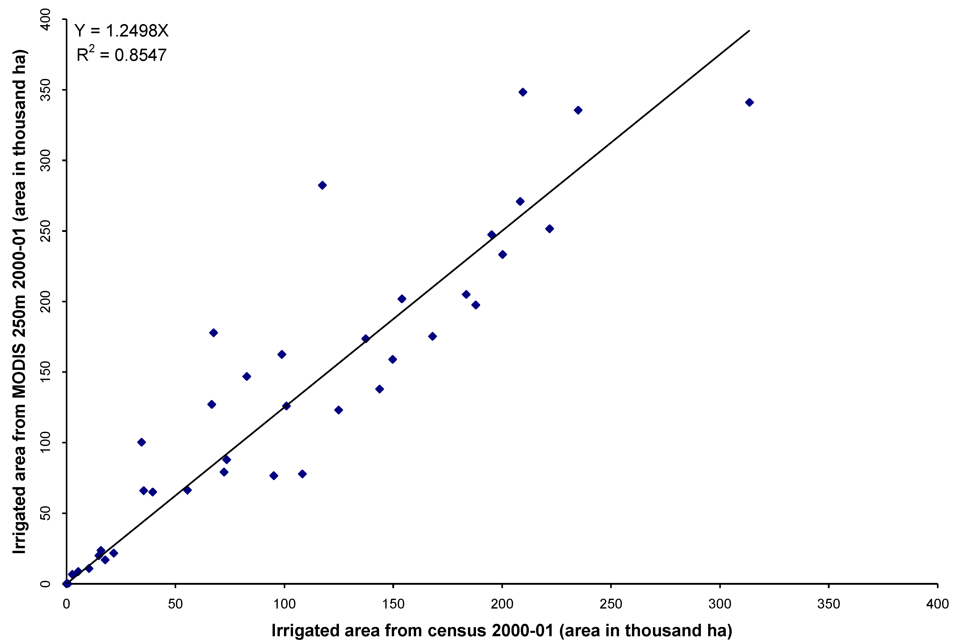
5.4. Comparisons with Census Data
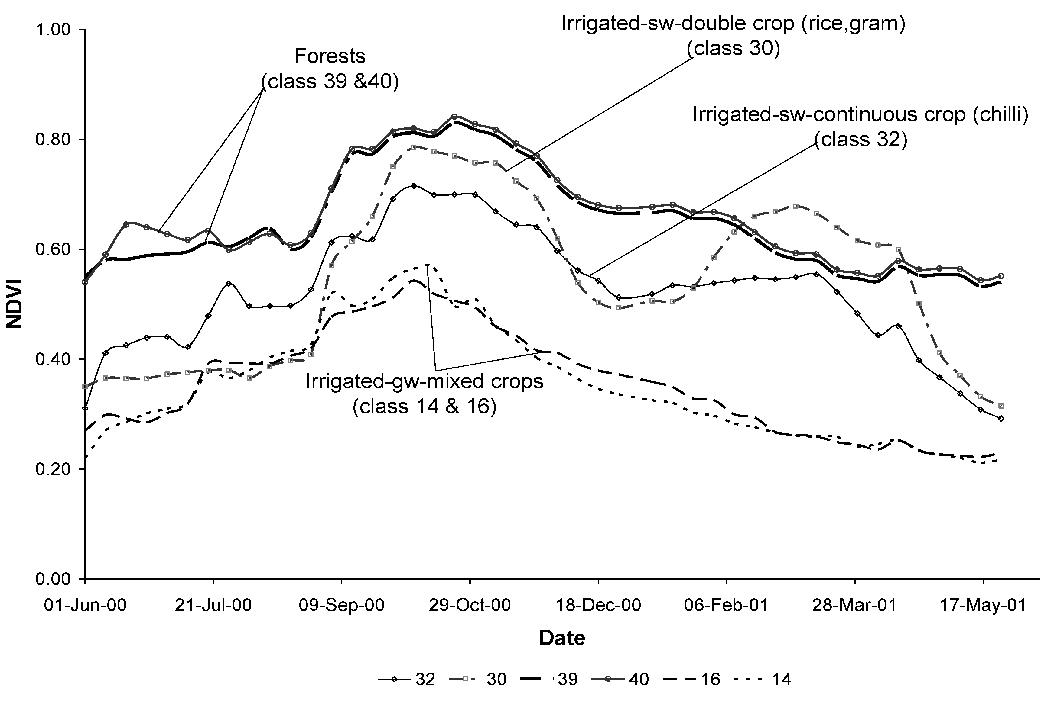
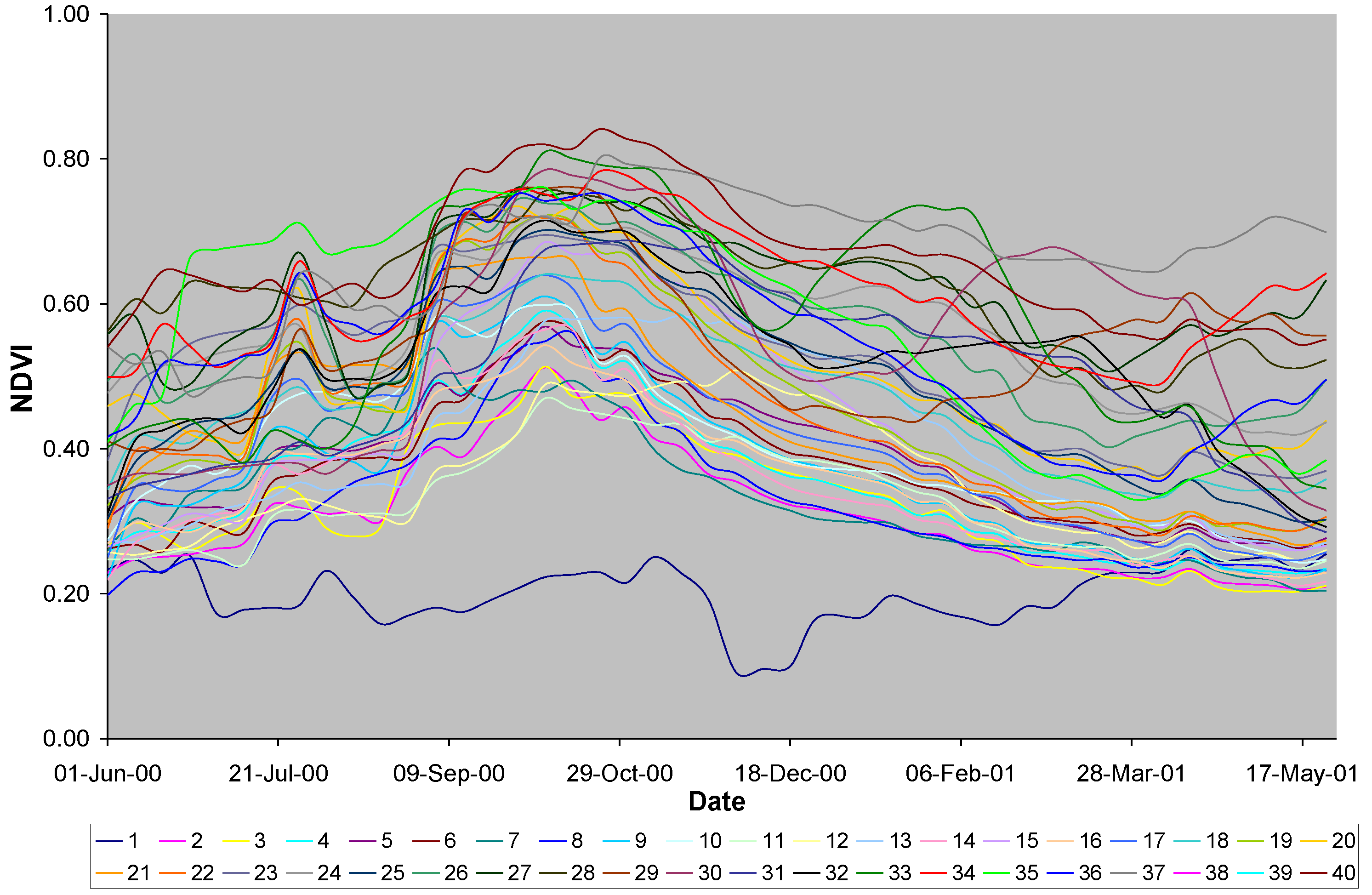
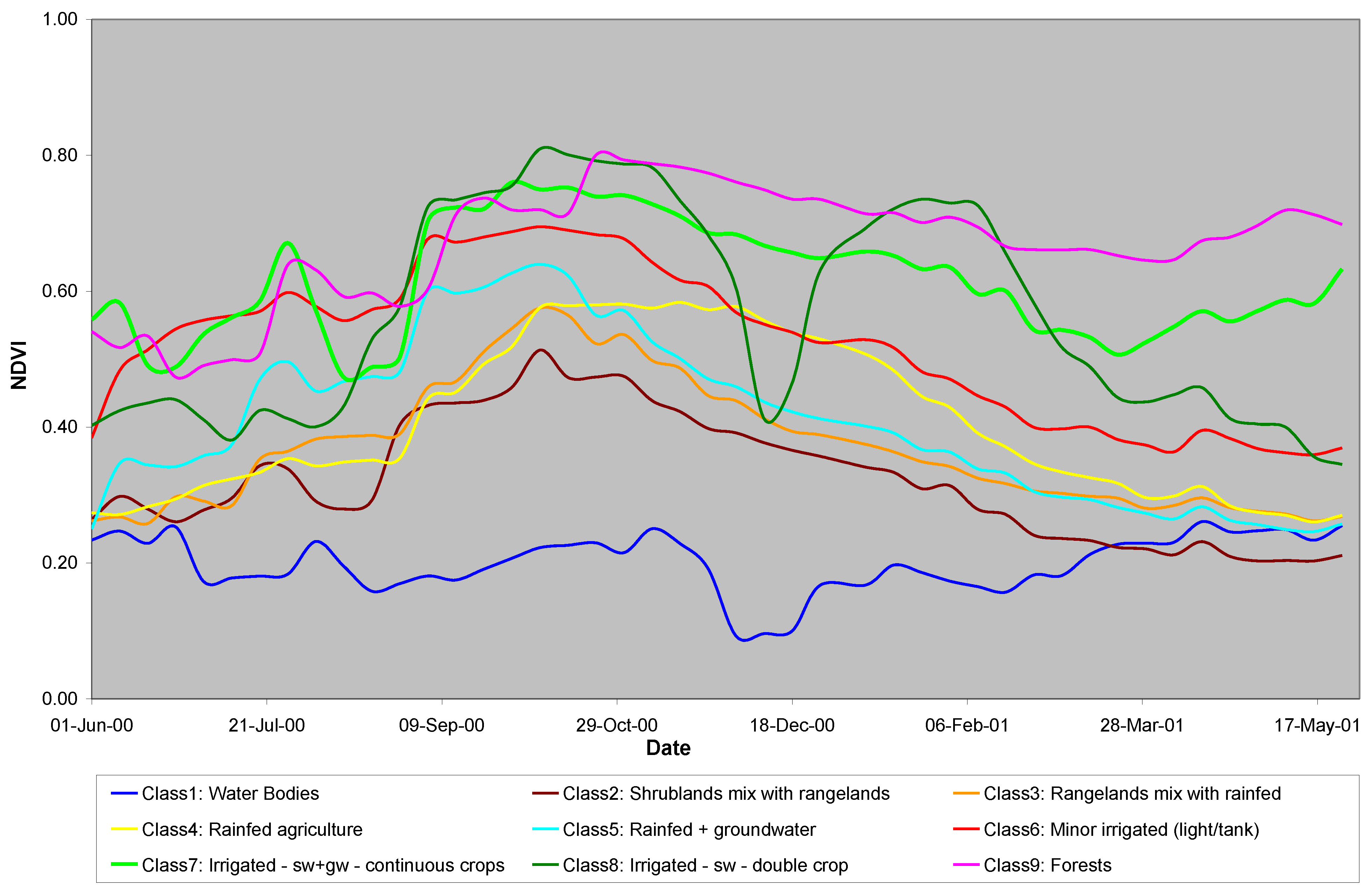
5.5. Vegetation Phenology of Ground Water and Surface Water Irrigated Areas
6. Conclusions
Acknowledgements
References
- Bhutta, M.N.; van der Velde, E.J. Equity of water distribution along secondary canals in Punjab, Pakistan. Irrig. Drain. Syst. 1992, 6, 161–177. [Google Scholar] [CrossRef]
- Gaur, A.; Biggs, T.W.; Gumma, M.K.; Parthasaradhi, G.; Turral, H. Water scarcity effects on equitable water distribution and land use in Major Irrigation Project—A Case study in India. J. Iirrig. Drain. Eng. 2008, 134, 26–35. [Google Scholar] [CrossRef]
- Shah, T.; Molden, D.; Sakthivadivel, R.; Seckler, D. The Global Ground Water Situation: Overview of Opportunities and Challenges; International Water Management Institute: Colombo, Sri Lanka, 2000. [Google Scholar]
- Velpuri, N.M.; Thenkabail, P.S.; Gumma, M.K.; Biradar, C.B.; Noojipady, P.; Dheeravath, V.; Yuanjie, L. Influence of resolution in irrigated area mapping and area estimations. Photogramm. Eng. Remote Sens. 2009, 75, 1383–1395. [Google Scholar] [CrossRef]
- Biggs, T.W.; Thenkabail, P.S.; Gumma, M.K.; GangadharaRao, T.P.; Turral, H. Vegetation phenology and irrigated area mapping using combined MODIS time-series, ground surveys, and agricultural census data in Krishna River Basin, India. Int. J. Remote Sens. 2006, 27, 21. [Google Scholar]
- Gumma, M.K.; Thenkabail, P.S.; Fujii, H.; Namara, R. Spatial models for selecting the most suitable areas of rice cultivation in the Inland Valley Wetlands of Ghana using remote sensing and geographic information systems. J. Appl.Remote Sens. 2009, 3, 033537. [Google Scholar] [CrossRef]
- Sellers, P.J.; Schimel, D. Remote sensing of the land biosphere and biogeochemistry in the EOS era: science priorities, methods and implementation. Global Planet. Change 1993, 7, 279–297. [Google Scholar] [CrossRef]
- King, M.D.; Closs, J.; Spangler, S.; Greenstone, R.E. EOS Data Products Handbook; Version 1; NASA Goddard Space Flight Center: Greenbelt, MD, USA, 2003.
- Thenkabail, P.S.; Schull, M.; Turral, H. Ganges and Indus river basin land use/land cover (LULC) and irrigated area mapping using continuous streams of MODIS data. Remote Sens. Environ. 2005, 95, 24. [Google Scholar]
- U.S. Geological Survey (USGS). Shuttle Radar Topography Mission (SRTM) “Finished” 3-arc second SRTM Format Documentation. Available online: http://gcmd.nasa.gov/records/GCMD_DMA_DTED.html (accessed on 6 November 2006).
- National Aeronautics and Space Administration (NASA). Moderate Resolution Imaging Spectrometer (MODIS). Available online: http://modis.gsfc.nasa.gov/data/dataprod/index.php (accessed on 21 August 2007).
- Gumma, M.K.; Thenkabail, P.S.; Iyyanki, M.V.; Velpuri, N.M.; GangadharaRao, T.P.; Dheeravath, V.; Biradar, C.M.; Nalan, A.S.; Gaur, A. Changes in agricultural cropland areas between a water-surplus year and water-deficit year impacting food security determined using MODIS 250 m time-series data and spectral matching techniques in the Krishna River Basin (India). Int. J. Remote Sens. 2011. [Google Scholar] [CrossRef]
- Huete, A.; Didan, K.; Miura, T.; Rodriguez, E. Overview of the radiometric and biophysical performance of the MODIS vegetation indices. Remote Sens. Environ. 2002, 83, 195–213. [Google Scholar] [CrossRef]
- Holben, B.N. Characteristics of maximum-value composite images from temporal AVHRR data. Int. J. Remote Sens. 1986, 7, 1417–1434. [Google Scholar] [CrossRef]
- Cihlar, J.; Xiao, Q.; Beaubien, J.; Fung, K.; Latifovic, R. Classification by progressive generalization: A new automated methodology for remote sensing multichannel data. Int. J. Remote Sens. 1998, 19, 2685–2704. [Google Scholar] [CrossRef]
- Achard, F.; Estreguil, C. Forest classification of Southeast Asia using NOAA AVHRR data. Remote Sens. Environ. 1995, 54, 198–208. [Google Scholar] [CrossRef]
- Cihlar, J. Land cover mapping of large areas from satellites: status and research priorities. Int. J. Remote Sens. 2000, 21, 1093–1114. [Google Scholar] [CrossRef]
- Thenkabail, P.S.; Biradar, C.M.; Noojipady, P.; Dheeravath, V.; Li, Y.; Velpuri, M.; Gumma, M.; Gangalakunta, O.R.P.; Turral, H.; Cai, X.; Vithanage, J.; Schull, M.A.; Dutta, R. Global irrigated area map (GIAM), derived from remote sensing, for the end of the last millennium. Int. J. Remote Sens. 2009, 30, 3679–3733. [Google Scholar] [CrossRef]
- Tucker, C.; Grant, D.; Dykstra, J. NASA’s global orthorectified Landsat data set. Photogramm. Eng. Remote Sens. 2005, 70, 313–322. [Google Scholar] [CrossRef]
- GoogleEarth. Available online: http://www.google.com/earth/index.html (accessed on 17 October 2007).
- Thenkabail, P.S.; GangadharaRao, P.; Biggs, T.; Krishna, M.; Turral, H. Spectral matching techniques to determine historical land use/land cover (LULC) and irrigated areas using time-series AVHRR pathfinder datasets in the Krishna River Basin, India. Photogramm. Eng. Remote Sens. 2007, 73, 12. [Google Scholar]
- Gopal, S.; Woodcock, C. Theory and methods for accuracy assessment of thematic maps using fuzzy sets. Photogramm. Eng. Remote Sens. 1994, 60, 8. [Google Scholar]
© 2011 by the authors; licensee MDPI, Basel, Switzerland. This article is an open access article distributed under the terms and conditions of the Creative Commons Attribution license (http://creativecommons.org/licenses/by/3.0/).
Share and Cite
Gumma, M.K.; Thenkabail, P.S.; Nelson, A. Mapping Irrigated Areas Using MODIS 250 Meter Time-Series Data: A Study on Krishna River Basin (India). Water 2011, 3, 113-131. https://doi.org/10.3390/w3010113
Gumma MK, Thenkabail PS, Nelson A. Mapping Irrigated Areas Using MODIS 250 Meter Time-Series Data: A Study on Krishna River Basin (India). Water. 2011; 3(1):113-131. https://doi.org/10.3390/w3010113
Chicago/Turabian StyleGumma, Murali Krishna, Prasad S. Thenkabail, and Andrew Nelson. 2011. "Mapping Irrigated Areas Using MODIS 250 Meter Time-Series Data: A Study on Krishna River Basin (India)" Water 3, no. 1: 113-131. https://doi.org/10.3390/w3010113