Modification of Aquifer Pore-Water by Static Diffusion Using Nano-Zero-Valent Metals

DCA Consultants Ltd., Haughend, Bridge of Earn Road Dunning, Perthshire, PH2 9BX, Scotland, UK
Water 2011, 3(1), 79-112; https://doi.org/10.3390/w3010079
Submission received: 5 December 2010
/
Revised: 24 December 2010
/
Accepted: 6 January 2011
/
Published: 11 January 2011
Abstract
:Sixteen static diffusion reactors containing n-ZVM (Fe0, Cu0, Al0) establish a common equilibrium redox (Eh-pH) trajectory which is directly linked to the aquifer pore volume, volume of injected n-ZVM, throughflow rate within the aquifer and time. The effect of NaCl and Ca-montmorillonite on the trajectory is considered. The trajectory can be directly linked to TDS (EC) and to the equilibrium removal of contaminants. In each example, the progressive oscillation between reduction and oxidation reactions (including Fenton reactions) creates the catalytic nuclei (and redox environment) required for the decomposition of organic pollutants and their reconstruction as simple alkanes and oxygenates.
Keywords:
zero valent iron; ZVI; zero valent metal; ZVM; TCE; DCE; desalination; decontamination; aquifer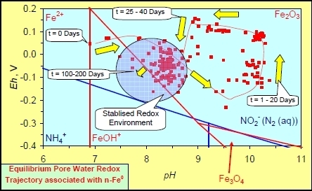
1. Introduction
Modification of the aquifer/reservoir redox (Eh, pH) environment and the formation of Fe ions (as active catalytic sites) are essential prerequisites [1] for in situ reservoir (i) decontamination/remediation, (ii) dechlorination of organic contaminants [1,2,3,4,5,6,7,8,9], (iii) desalination, and (iv) catalytic oil restructuring (e.g., as part of an enhanced oil recovery scheme).
A number of pilot projects have used (i) n-Fe0 injection (IZVM) [1,10,11,12,13,14,15,16] and (ii) the placement of permeable reactive barriers (PRB) containing n-Fe0 within flow paths located in an aquifer to modify the pore-water redox by static diffusion [1,17,18,19,20,21,22,23]. Remediation is a direct result of the change in redox environment. The equilibrium concentration of each contaminant varies with Eh/pH.
Flow through permeable, or semi-permeable, barriers is not homogenous (e.g., PRB). Flow is characterized by the development of mesopores, macropores and natural pipes [1,24,25,26,27] where only a small part of the throughflow has direct contact with the matrix/particles of the barrier [25,26,27]. The principal mechanism for redox modification of the throughflow is static diffusion within the macropores.
ZVM research has focused on determining n-ZVM kinetic reaction rates [28] over a period of minutes or hours [29,30] or months [28]. Reaction kinetics are important in a simple closed system reactor design, but are largely irrelevant in the design of IZVM (injected ZVM program) or a ZVM PRB in a more complex open or semi-open aquifer buffer environment.
ZVM aquifer geoengineering requires [1] an understanding of the inter-relationship between pH, Eh, and space velocity (SV) during the design of a n-ZVM permeable reactive barrier (PRB) or injected ZVM (IZVM) program. This is to allow quantitative modelling of the expected changes in aquifer redox environment as a function of time, injection/infiltration rates, and aquifer flow rates.
The impact of changing water salinity, or the presence of clays, on the inter-relationship between pH, Eh, and space velocity is poorly understood. Following n-ZVM injection, the aquifer Eh, pH varies with time and SV [12,14]. Static diffusion studies [1] using m-ZVM have established a redox trajectory which can be directly linked to time and SV. The linkage to SV allows continuous flow reactors to target a constant product water Eh, pH, with a consistent level of water treatment. The same strategy cannot be applied to fixed bed reactors containing n-ZVM (due to loss of permeability with time) but may be applicable to fluidised bed reactors or slurry reactors containing n-ZVM. These reactors can contain clays (e.g., montmorillonite). The large pore size and particle size associated with m-ZVM results in a relatively high degree of variance associated with the redox trajectory (with time and SV) [1]. n-ZVM has a smaller particle size and pore size. In a continuous flow fixed bed reactor, this results (when compared with m-ZVM) in a higher Eh and pH associated with a specific flow rate and SV. This, in turn, reduces both the level of water treatment control and the types of contaminant which may be removed using a continuous flow fixed bed water treatment reactor.
This study seeks to address these issues by investigating the change in pore-water redox (with n-ZVM, salinity and clay presence) associated with static diffusion using sixteen static diffusion micro-reactors, SDR, (MR1-MR16). The observed relationships between SV (Equations 1 and 2), and Eh, pH, EC and water salinity + clay presence can be used to design a geoengineered redox transformation of an aquifer. They can also be used to predict the expected behavior of pore-water modification programs associated with injected n-ZVM and n-ZVM permeable reactive barriers. Similar relationships for m-ZVM have been presented elsewhere [1] together with a detailed methodology for their application in designing ZVM aquifer treatment.
Vw = Water volume, m3; Vc = nano-metal volume, m3; Rt = Average time spent by each m3 of water in the reactor, h. For a static water body Rt = time; For a flowing water body within a aquifer, SV (m3 H2O h−1 m−3 n-ZVM) can be calculated as
where Vwf = Flowing water volume, m3 h−1.
SV (m3 H2O h−1 m−3 n-ZVM) = (Vw/Vc)/Rt
SV (m3 H2O h−1 m−3 n-ZVM) = (Vwf/Vc)
2. Materials and Methods
Measurements were made of EC, Eh, pH, and temperature using Hanna HI-98120 (ORP/Temperature, Hanna Calibration Number = 24230), Hanna HI-98129 (pH, EC, TDS, Temperature; Hanna Calibration Number = 33999). Hi-98120 is factory calibrated. HI-98129 was calibrated using Hanna test reagents (pH buffer solutions 4.01, 7.01, 10.01 (HI-7004, HI-7007, HI-7010) and conductivity solution 1.413 mS cm−1 (HI-7031)). Eh298.15K calculated from ORP as Eh = ORP (298.15/To). To = measured temperature, K. TDS (Total dissolved solids, ppm) = EC (mS cm−1) × F × 103. F = a factor (e.g., 0.5). The untreated test water (pH = 6.2–7.1, Eh = 0.034–0.185 V) was extracted from an unconfined infiltration reservoir in fractured Devonian (Old Red Sandstone Volcanic Series, Ochil Hills, UK) basalts.
2.1. Experimental Micro-SDR
Static diffusion was examined in four different environments:
- Fresh water containing n-ZVM + Ca-montmorillonite (MR9–MR11)—Figure A9, Figure A10 and Figure A11 in Appendix.
- Saline water containing n-ZVM + Ca-montmorillonite (MR12–MR16)—Figure A12, Figure A13, Figure A14, Figure A15 and Figure A16 in Appendix.
Each micro-SDR (0.07 m internal diameter) contained 0.0032 m3 H2O [(MR1-5); 0.002 m3 H2O (MR6-16)] with nano-zero valent metal (n-ZVM) placed at the base of the reactor. The n-ZVM occupied between 1.2% (MR1, MR2, MR6) and 4.4% (MR16) of the stored water volume. The standard ZVM quantities used in each SDR are Fe0 = 18 gms; Cu0 = 2.8 gms; Al0 = 4.6 gms; Ca-montmorillonite = 12.5 gms. The n-ZVM is constructed as ground high purity metal (<66,000 nm). The Ca-montmorillonite was added as anhydrous granules (1–5 mm). This clay swells and flocculates in the presence of water to create a clay containing n-ZMV. The static diffusion test results are placed in Appendix, Figures A1–A16. The water used in MR6 (Figure A6in Appendix ) contains dissolved organic matter (DOM) derived from chicken manure fertiliser.
2.2. Characterization of n-ZVM
The n-ZVM powders used are illustrated elsewhere [1] and have a particle size of 44,000–66,000 nm (mesh size: BSS = 240–350; Tyler = 250–325; US = 230–325). The surface area of the n-ZVM used in this study varies from 0.00289–0.01732 m2 g−1 (Table 1). This type of powder is produced by grinding metal. Most n-ZVM used in water treatment is produced by precipitating n-ZVM onto a skeleton in order to maximize n-ZVM surface area.
Consequently the surface areas of the n-ZVM used in this study are substantially lower than the typical BET surface area of 35 m2 g−1 precipitated n-Pd/Fe (median particle size = 60 nm) [31,32] and commercially available n-Fe powder (<10 nm), surface area of 0.9 m2 g−1 [32]. Most precipitated n-Fe0 powders and powders derived from the reduction of ferrous iron used in water treatment have a BET surface area of about 30 m2 g−1 [33]. Larger grain size powders (e.g., 800–2800 nm) may have surface areas of 6–15 m2 g−1 [34]. Surface areas of 50–600 m2 g−1 are associated with n-Fe0 produced by reduction of iron oxide nanoparticles (<30 nm)[35].

Table 1.
Relationship between Fe0 particle size and surface area (m2 g Fe0), where the n-Fe0 is produced by grinding Fe0. 1 nm = 10−9 m. The nano-particles examined in this study have a grain size of 0.044–0.066 mm.
| Spherical Form | Cube Form | ||||||
|---|---|---|---|---|---|---|---|
| m | mm | m2 | g | m2 g Fe0 | m2 | g | m2 g Fe0 |
| 2.00 10−03 | 2 | 1.26 10−05 | 3.30 10−02 | 0.00038 | 6.00 10−06 | 6.30 10−02 | 0.00010 |
| 1.00 10−03 | 1 | 3.14 10−06 | 4.12 10−03 | 0.00076 | 1.50 10−06 | 7.87 10−03 | 0.00019 |
| 5.00 10−04 | 0.5 | 7.85 10−07 | 5.15 10−04 | 0.00152 | 3.75 10−07 | 9.84 10−04 | 0.00038 |
| 1.00 10−04 | 0.1 | 3.14 10−08 | 4.12 10−06 | 0.00762 | 1.50 10−08 | 7.87 10−06 | 0.00191 |
| 6.60 10−05 | 0.066 | 1.37 10−08 | 1.19 10−06 | 0.01155 | 6.53 10−09 | 2.26 10−06 | 0.00289 |
| 4.40 10−05 | 0.044 | 6.08 10−09 | 3.51 10−07 | 0.01732 | 2.90 10−09 | 6.71 10−07 | 0.00433 |
| 1.00 10−06 | 0.001 | 3.14 10−12 | 4.12 10−12 | 0.76200 | 1.50 10−12 | 7.87 10−12 | 0.19050 |
| 1.00 10−07 | 0.0001 | 3.14 10−14 | 4.12 10−15 | 7.62002 | 1.50 10−14 | 7.87 10−15 | 1.90500 |
| 1.00 10−08 | 0.00001 | 3.14 10−16 | 4.12 10−18 | 76.20015 | 1.50 10−16 | 7.87 10−18 | 19.05004 |
2.2.1. Negative activation energies
Historically n-ZVM is treated as a catalyst whereby the effectiveness of the n-ZVM is assumed to be a function of the n-ZVM surface area (m2 g Fe0). The assumption made (in accordance with standard catalyst theory) is that increasing surface area will increase the availability of active sites and the ability for adsorption/desorption reactions to occur on/in the catalyst. These reactions are typically characterized by positive activation energies. It has been demonstrated [1] that n-ZVM associated reactions are essentially fluid phase electrochemical reactions (or contact surface reactions) where the principal controls on remediation are the H+:OH− ratio (pH) and the HO2−:OH− ratio (Eh) in the fluid. Eh and pH alteration of pore water chemistry is electrochemical [1] and not purely catalytic.
The low surface area of the n-ZVM used in this study (Table 1) will result in a domination of fluid, electrochemical (and surface) reactions. The principal control on remediation is switched from catalytic adsorption/desorption reactions over the n-ZVM surface area to the impact of the electrochemical environment in the fluid created by the presence of the n-ZVM. This forces reaction selectivity towards reactions which have negative activation energies (e.g., reaction rate increases with decreasing temperature) and fluid/surface reactions which involve OH, O, methylene and halogen species (i.e., reactions which are directly controlled by pH and Eh). Negative activation energies are also associated with the interaction of methylene (e.g., ZVM-CH3) and halogen species (e.g., HCl, HBr, etc.) to produce methane + halogen [36] and the breakdown of n-alkanes [37].
The addition of OH or O2 (as H2O2 or HO2-) to an organic double bond results [38] in the virtually instantaneous breakdown of alkenes [38,39]. Similar observations have been made [39] for the break down (by OH addition) of carbonyls (e.g., aldehydes), haloethanes, and aromatic hydrocarbons [39] and reconstruction of CO to CO2 (n-ZVM-OH + CO = n-ZVM + H + CO2) [40]. The latter reaction has a negative activation energy in the presence of water, but may have a positive activation energy when water is absent [40]. This remediation is accelerated by:
- Increasing the availability of OH− (i.e., increasing pH as the concentration of OH- (Mol L−1) = 10(14−pH)).
- Increasing the rate of degradation of HO2− to H2O + 0.5O2 (i.e., decreasing Eh, as Eh is a direct measure of the ratio [HO2−]:[OH− + HO2−]).
Studies using m-ZVM [1] have demonstrated that Fe0 can adjust the fluid pH from <7 to >11, and that bi or tri metal combinations of m-ZVM will maximize the rate of Eh reduction (and O2 evolution). Eh reductions may fall in the range 0.3 to 0.8 V. The fluid phase reaction routes which result may (for a specific pH) be dependent on Eh. For example where the water contains CO2 and H+ ions, then for pH = 7, the relationships provided in Equation 3 may apply [41]:
CO2 + 2H+ + 2e− = HCOOH Eh = −0.61 V
CO2 + 2H+ + 2e− = CO + H2O Eh = −0.53 V
CO2 + 6H+ + 6e− = CH3OH + H2O Eh = −0.38 V
CO2 + 2H+ + 2e− = CO + H2O Eh = −0.53 V
CO2 + 6H+ + 6e− = CH3OH + H2O Eh = −0.38 V
The reaction product is a function of Eh. CO2 in the water will be reduced to CO or hydrocarbons in the remediation zone (Equation 3). The CO product will maintain the ZVM in a reduced state [40].
2.3. Dissolved Organic Matter (DOM)
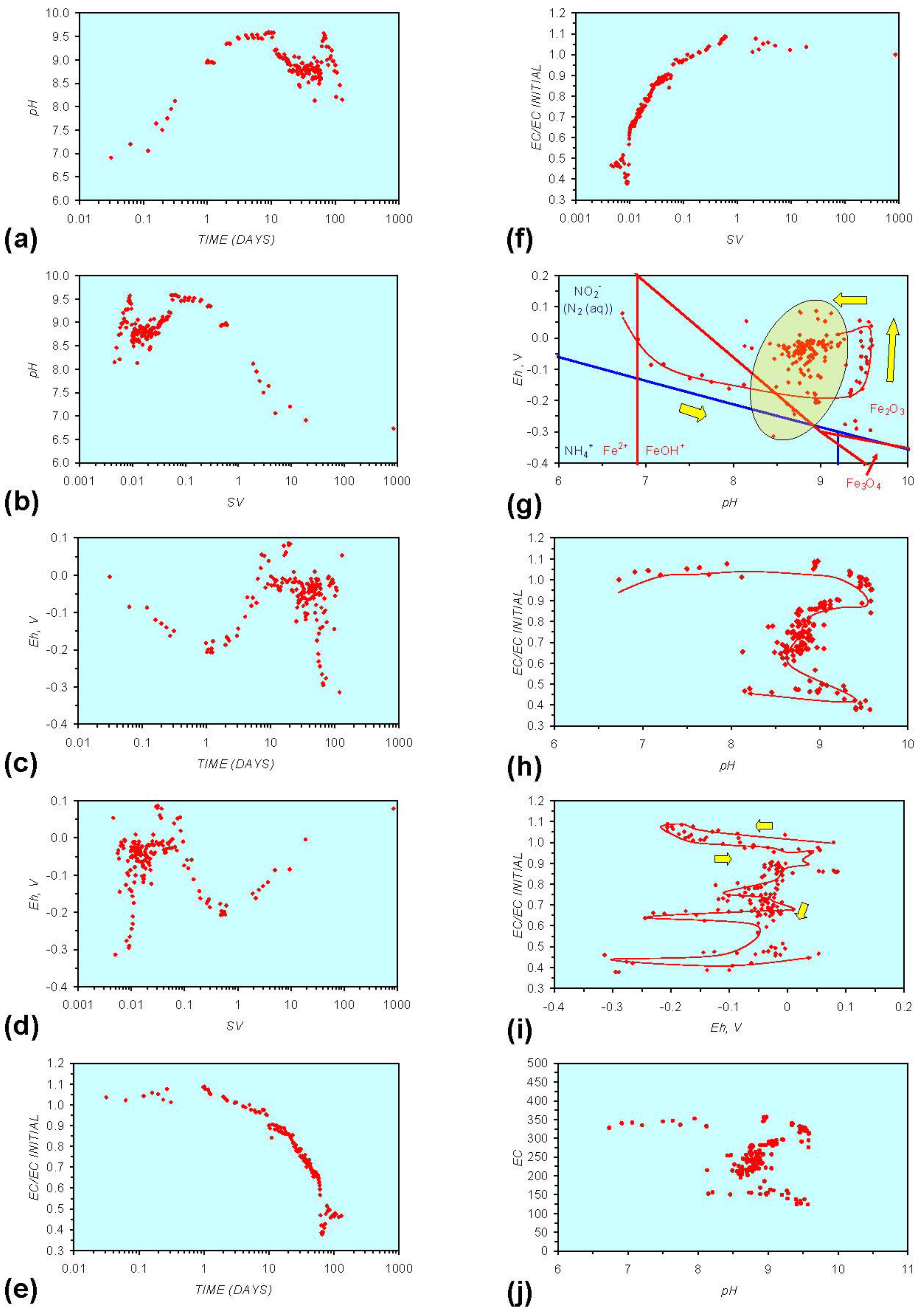
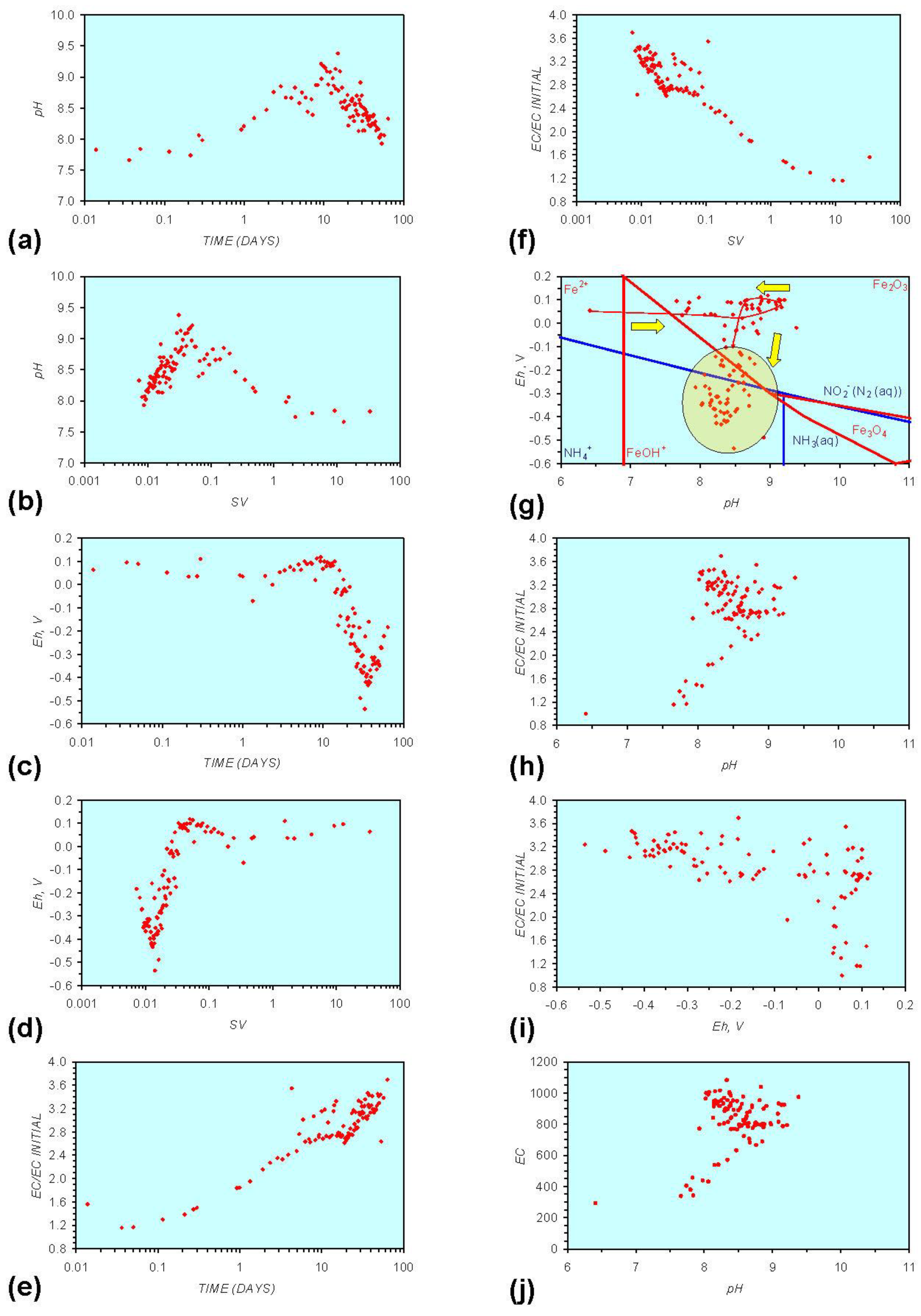
Pore-water redox modification by static diffusion using n-Fe0 was analyzed (MR1, Figure A1 in Appendix) using fresh water (Figure 1). The experiment was repeated (MR6, Figure A6 in Appendix) using water containing dissolved organic matter (DOM). The water for MR6 was prepared using a commercial dried (sterilized) granulated chicken manure fertilizer. The fertilizer was dissolved in the water and the solute was added to the ZVM. The solute was diluted to ensure an initial EC of <2000 μS cm−1 (Figure A6 in Appendix).
The fertilizer contained 4.5% N (as ammonium salts and nitrates), 3.5% P (as phosphates and phosphenes), 2.5% K, 1% Mg, 0.5% S (as SO4), 9% Ca + traces of Fe, Mn, Mo, Cu, Zn. The residue is organic matter. The mineral composition of this chicken manure is typical [42]. It is established that chicken manure increases pH [43,44] (by up to about 5 units [44]) and increases EC substantially [43].
Similar observations have been made with raw cow manure, where pH increases to 7–9 units and Eh decreases to between −0.07 and −0.37 V [45,46]. Anaerobic digestion within the manure can result in acidification (i.e., pH < 7) and a decrease in Eh (i.e., <−0.5 V) [47].
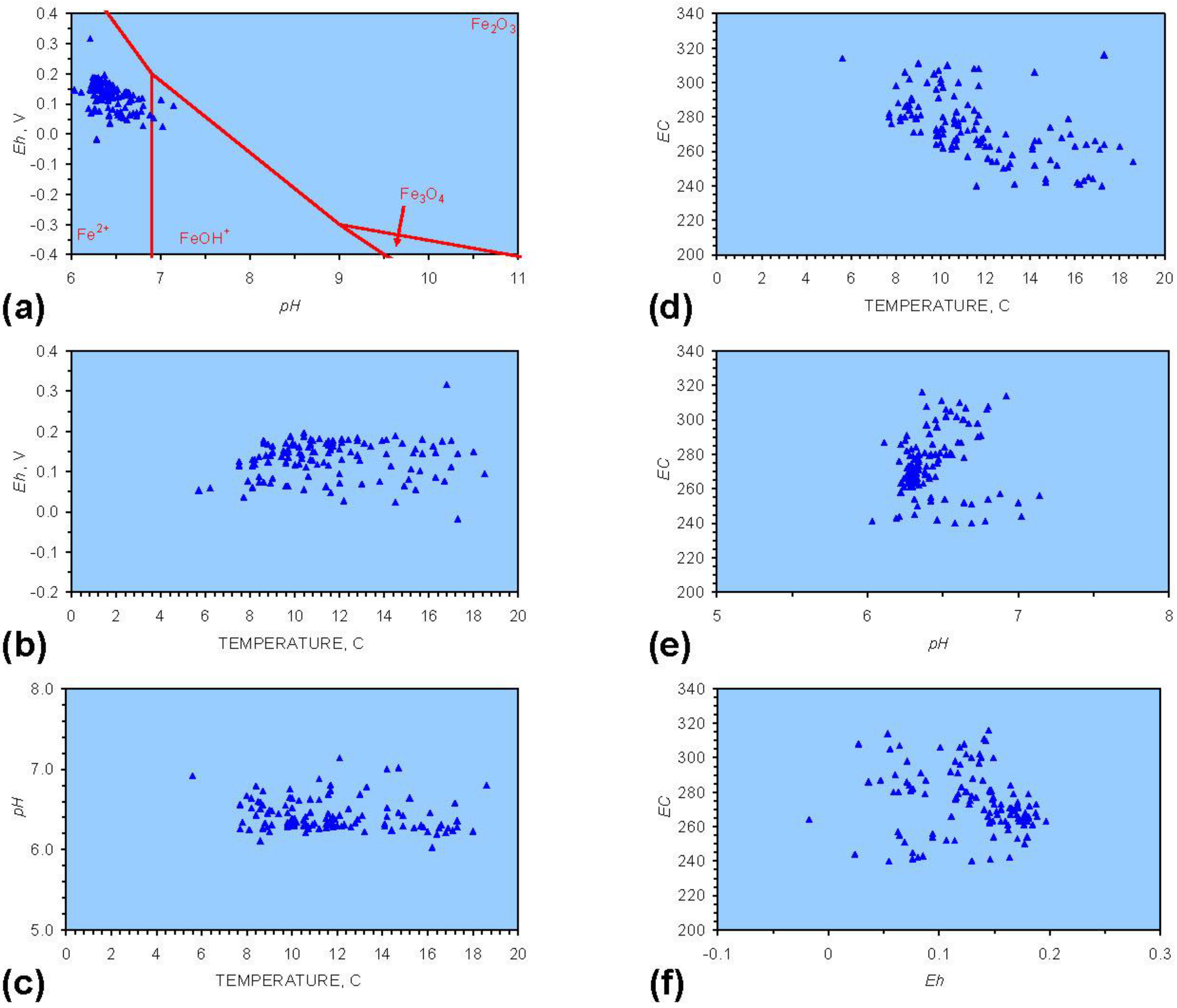
Figure 1.
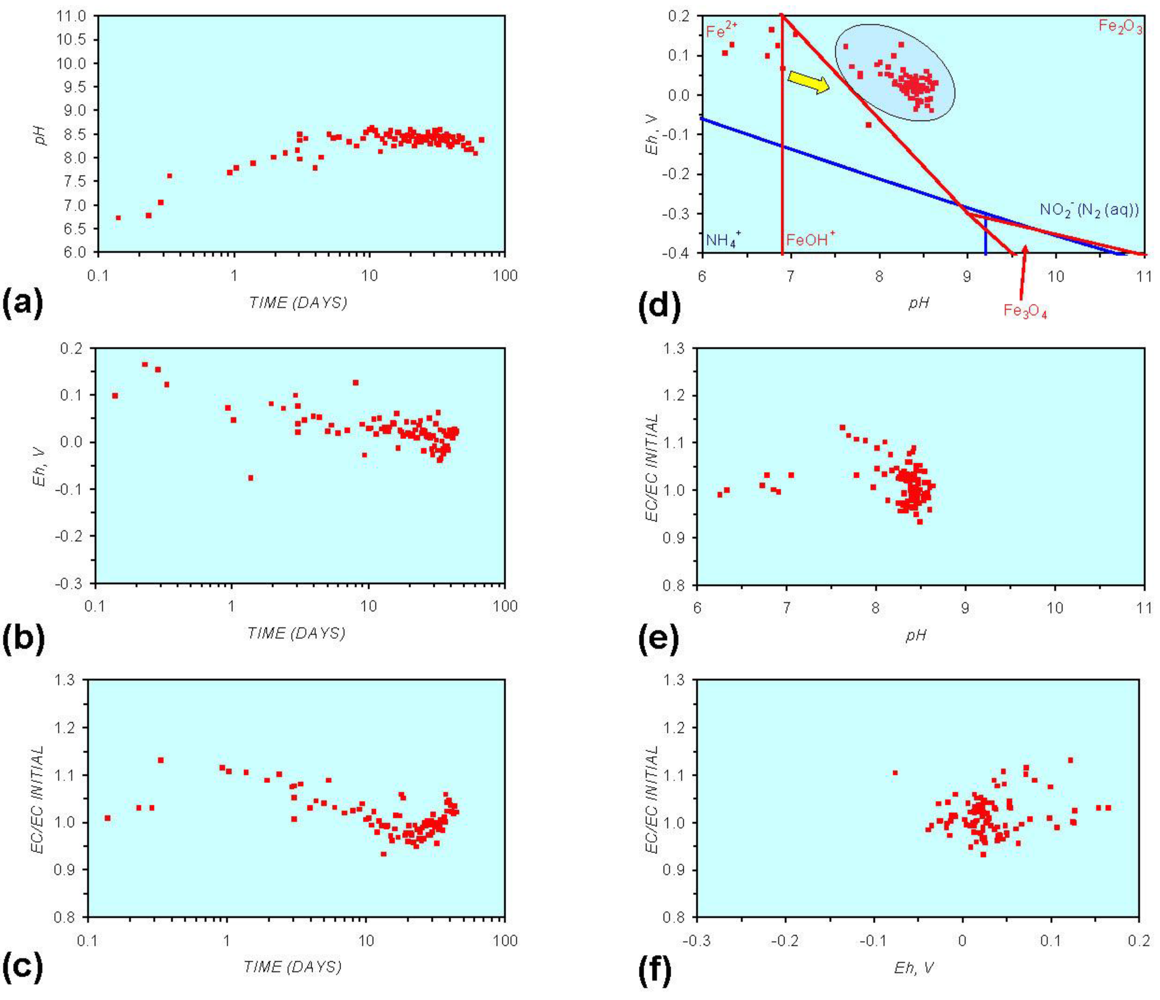
Eh-pH relationship for feed water. (a) natural variation in groundwater mound (March–July 2010). Redox fences for Fe from [1]; (b) Eh vs. Temperature; (c) pH vs. Temperature; (d) EC (μS cm−1) vs. temperature; (e). EC (μS cm−1) vs. pH; (f) EC (μS cm−1) vs. Eh. Temperatures are the sampled temperature of water abstracted from the groundwater mound.
Figure 1.
Eh-pH relationship for feed water. (a) natural variation in groundwater mound (March–July 2010). Redox fences for Fe from [1]; (b) Eh vs. Temperature; (c) pH vs. Temperature; (d) EC (μS cm−1) vs. temperature; (e). EC (μS cm−1) vs. pH; (f) EC (μS cm−1) vs. Eh. Temperatures are the sampled temperature of water abstracted from the groundwater mound.

3. Experimental Results: n-ZVM + Water
3.1. Source Water
The source infiltration groundwater mound has an Eh-pH relationship, which varies over the course of a year (Figure 1a, 1b, 1c). The EC (i.e., TDS) decreases with increasing temperature (Figure 1d). EC is not related to pH or Eh (Figure 1e, 1f).
The experiments were designed to determine if:
- Addition of n-ZVM resulted in a significant change in EC, pH or Eh.
- The change in Eh, EC, pH followed a specific (and predictable) pattern as a function of contact time with the ZVM (e.g., SV).
3.2. Experimental Results
The experimental results are presented in Figures A1–A16 (Appendix) as a series of relationships vs. time (or space velocity) and a series of crossplots. These establish that Eh, pH and EC change with time in the presence of ZVM or Ca-montmorillonite, and that the presence of NaCl impacts on the Eh, pH and EC. These changes can be related to a series of regression relationships vs. time (or space velocity). They can therefore provide an indication of the modified redox environment and its changes with time. The methodology required to translate the graphical data into modeled aquifer performance results (for an aquifer remediation program) for the design of permeable reactive barriers and aquifer remediation programs is provided elsewhere [1].
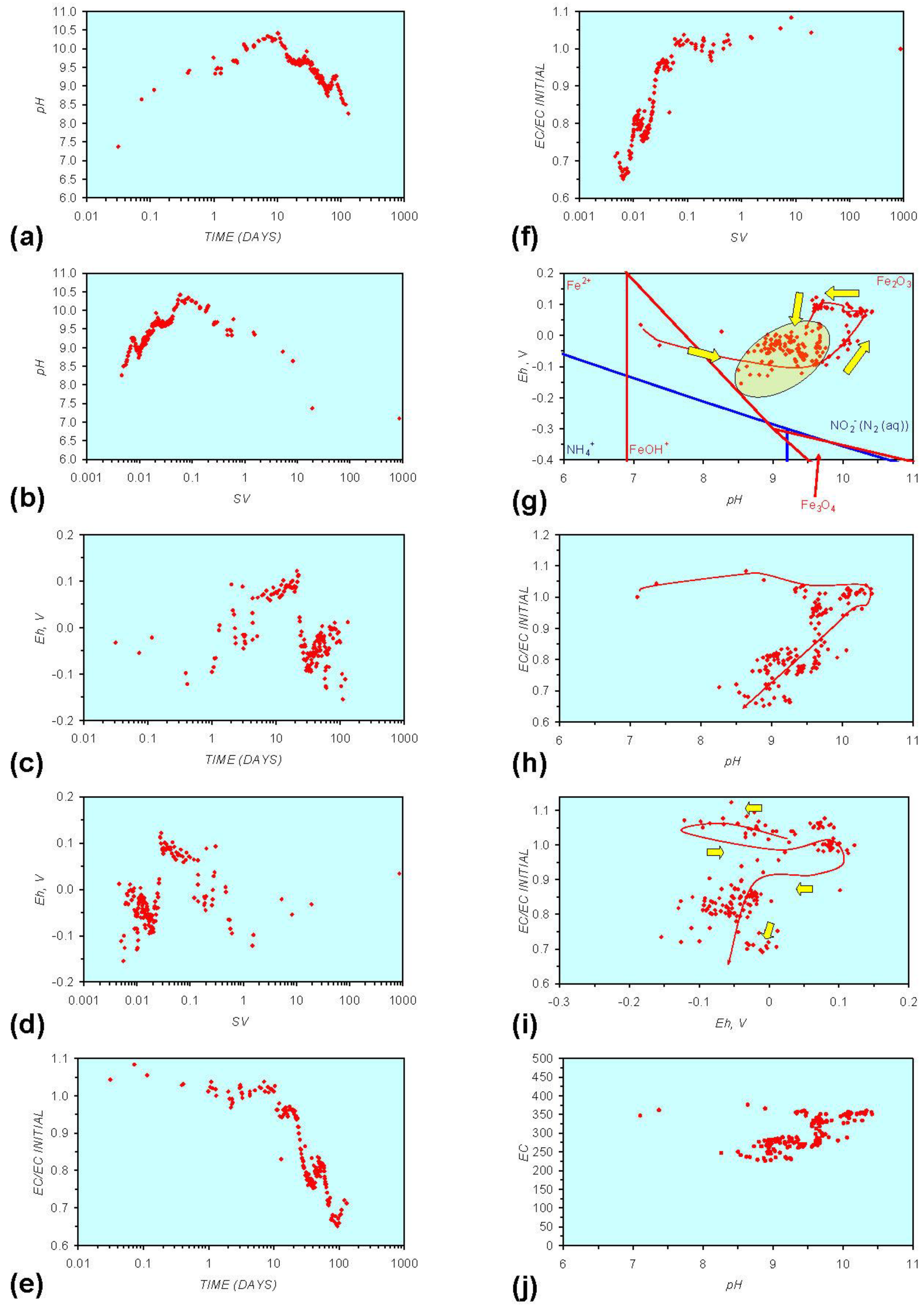
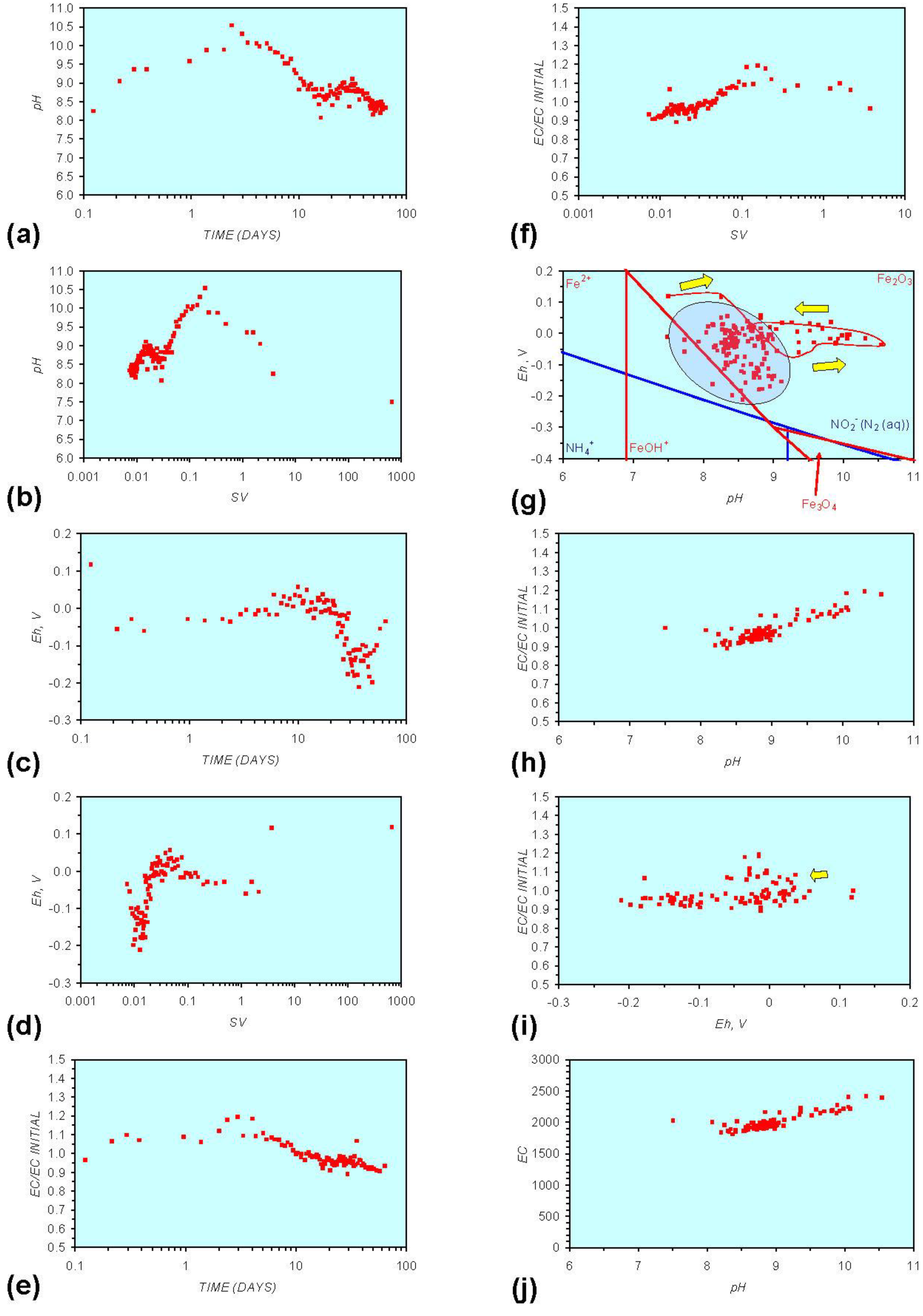
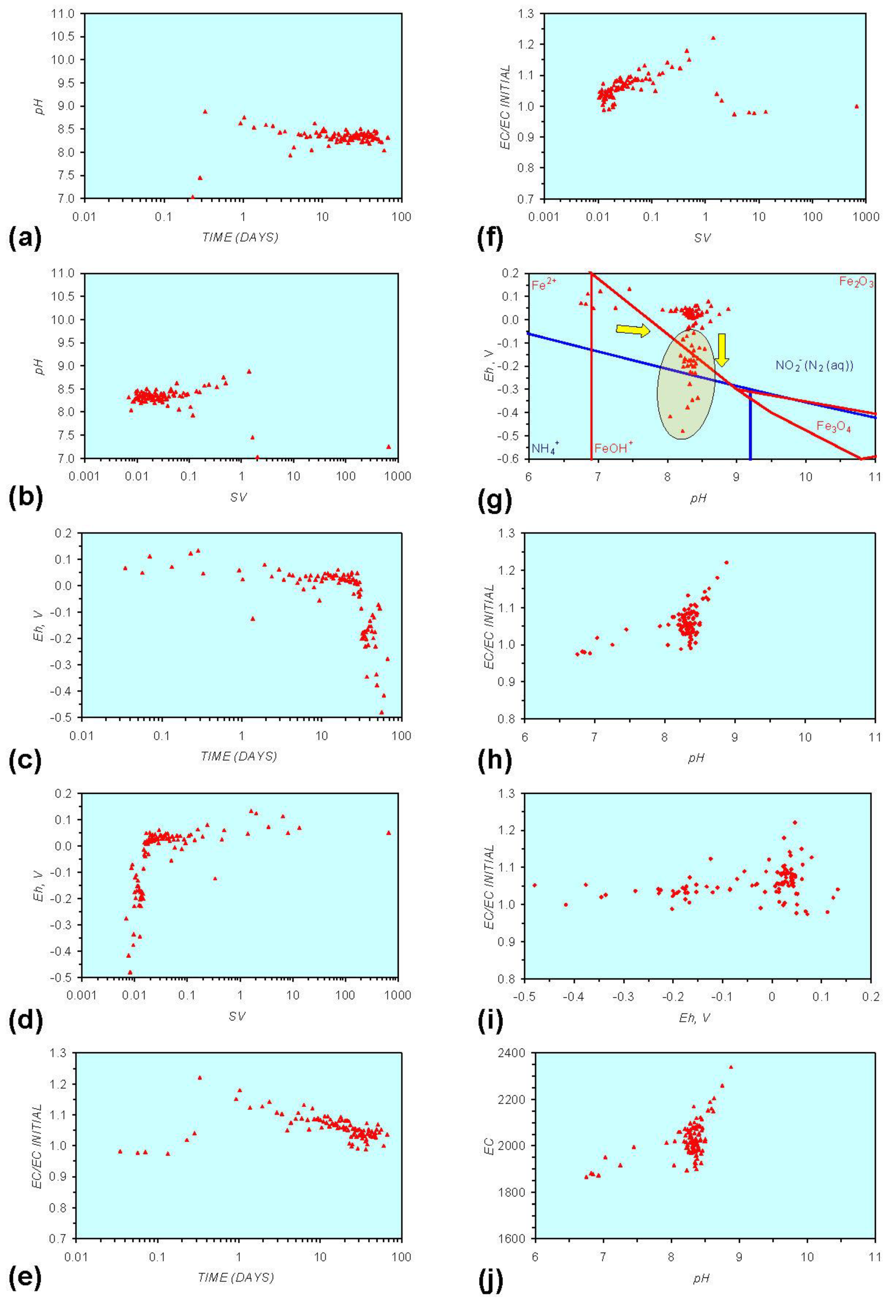
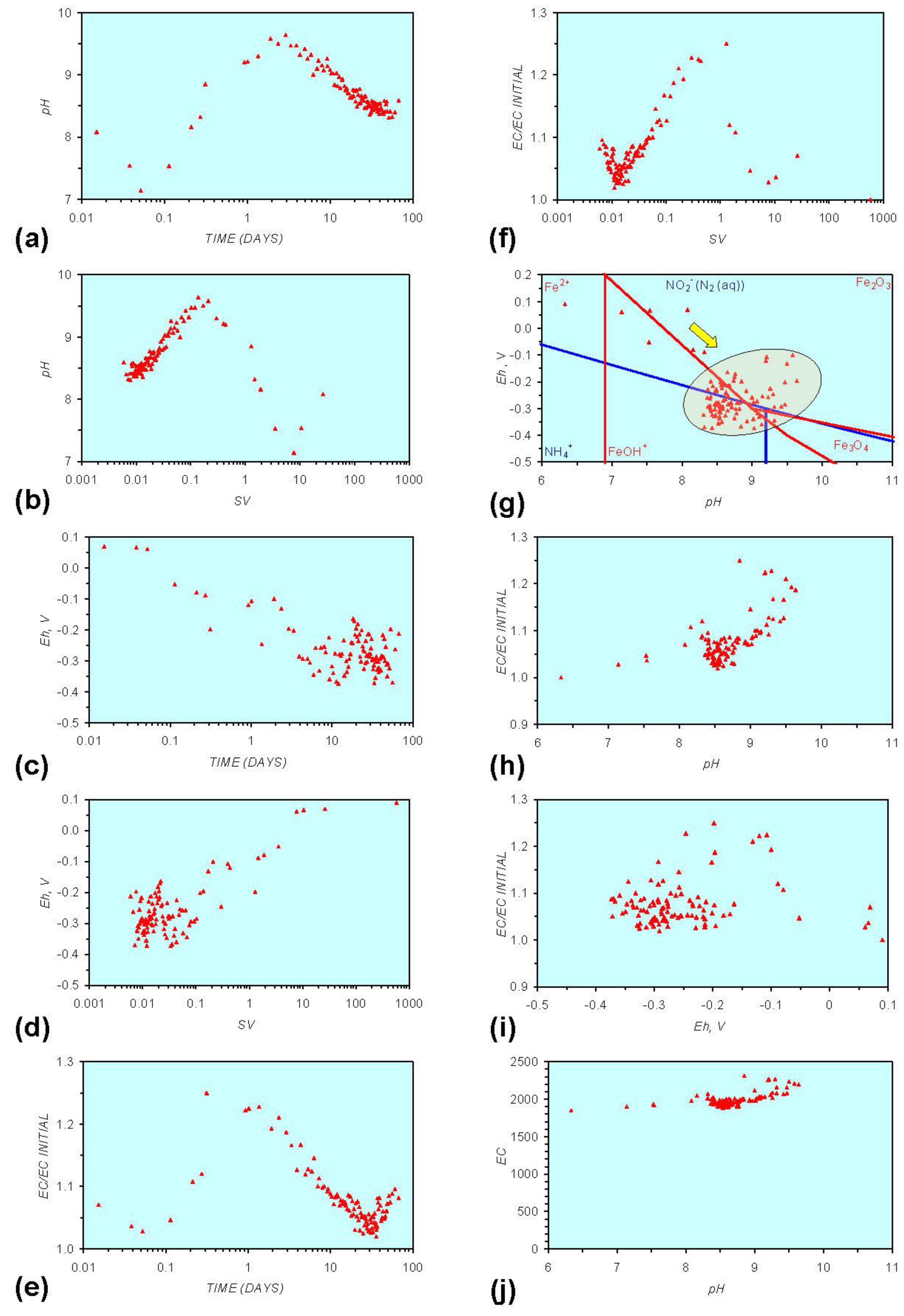
In each example containing n-Fe0 the same general pattern is replicated (e.g., Figure A1g in Appendix):
- (i)
- An initial rapid increase in pH (to around pH = 10) is accompanied by a decrease in Eh.
- (ii)
- This is followed by a stabilization in pH (at around pH = 10) and a rise in Eh.
- (iii)
- This is then followed by a stabilization of Eh (e.g., Eh = 0.05 V) and a decrease in pH to a base level (e.g., pH = 8–9).
The pH then remains constant at the base level (e.g., pH = 8–9) and the Eh then starts to decline to a base level, (e.g., Eh ≤ −0.1 V) to form a stabilized redox environment (SRE).
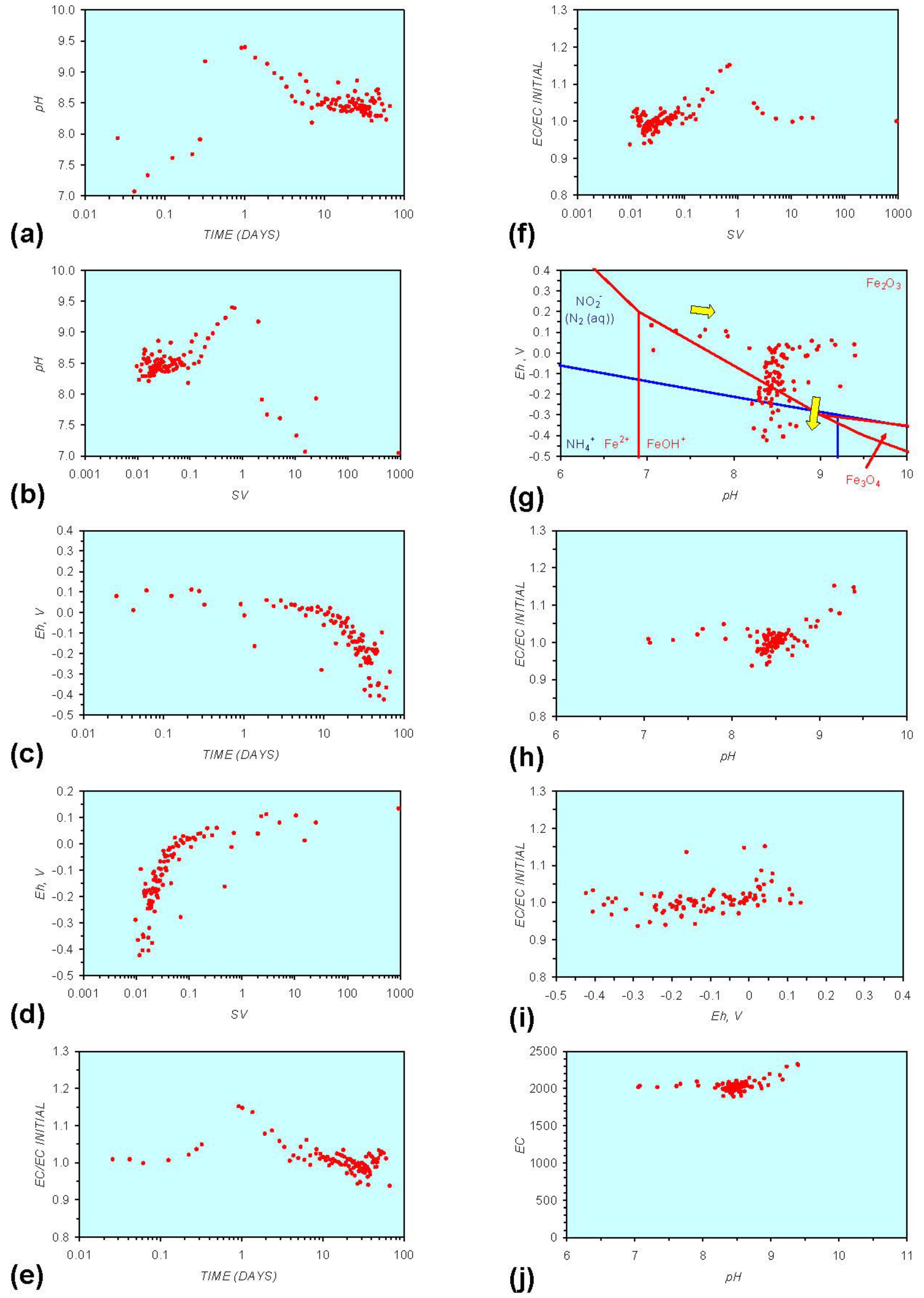
This general pattern is illustrated in Figure A1g, and is present in all the test samples containing n-Fe0. The test sample containing only n-Al0 (Figure A2g in Appendix) shows a similar pattern. However, the cycle continues with an increase in pH (from about 7.5 to about 8.5, Figure A2g in Appendix), followed by pH stabilization and a rise in Eh.
The general patterns associated with n-Al0 (Figure A2 in Appendix) can be compared directly with the Ca-montmorillonite patterns (Figure A9 and Figure A12 in Appendix). In freshwater these show an initial decrease in Eh (or stable Eh) accompanied by an increase in pH. This is then followed by an increase in Eh and decrease in pH. Ca-montmorillonite contains Al cations. In saline water, the pH increase is accompanied by a stable Eh (Figure A13 in Appendix).
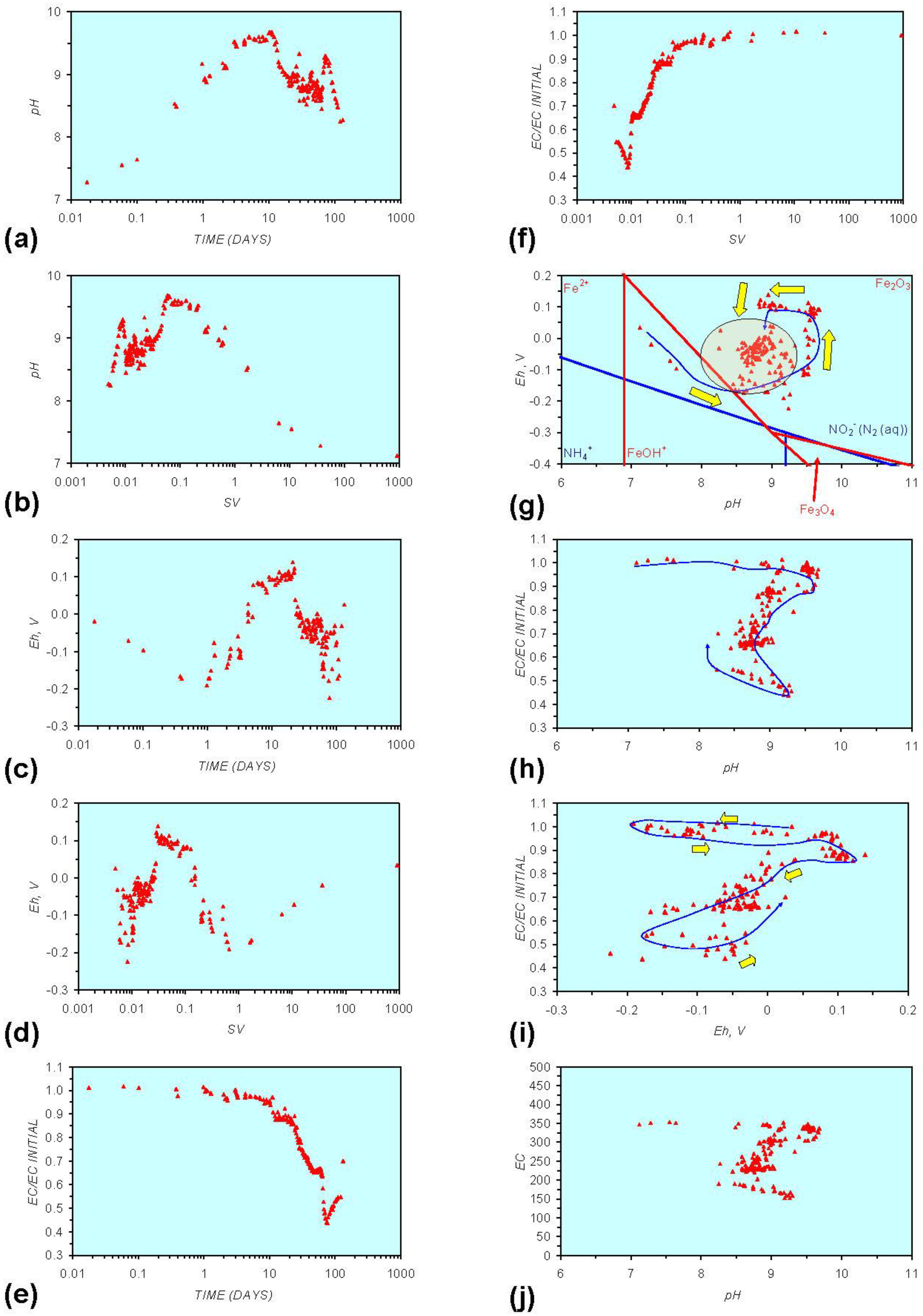
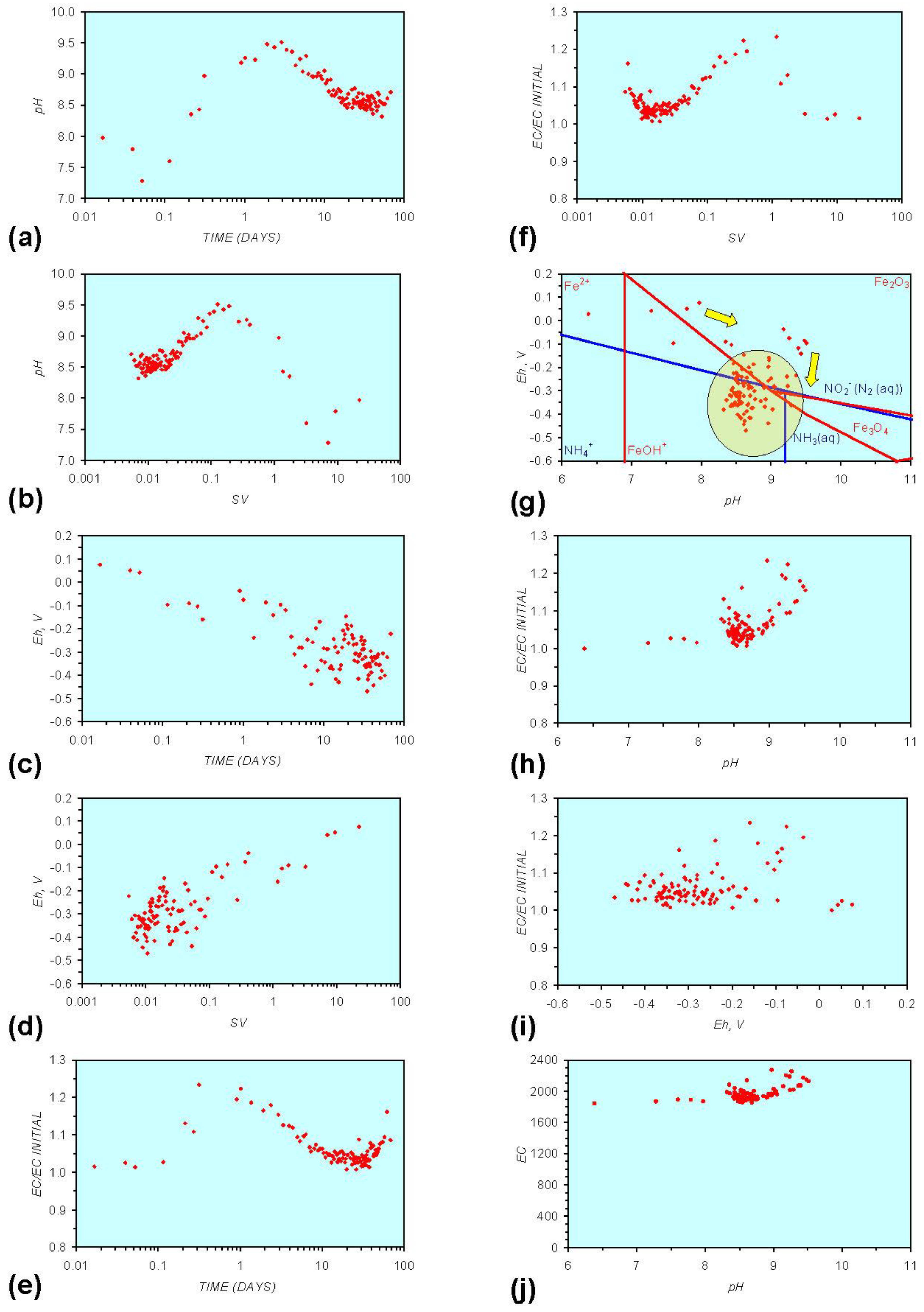
Figure A1 to Figure A5 demonstrate that the impact of adding different n-ZVM to n-Fe0 is to reduce the maximum pH achieved in the redox cycle and adjust the stabilized pH and Eh (SRE) over the longer term (compare Figure A1g, Figure A3g, Figure A4g and Figure A5g in Appendix). The presence of dissolved organic matter (DOM), while affecting the initial starting pH, Eh and EC, does not appear to affect the overall redox cycle (Figure A6g in Appendix). The SRE and redox trajectory (associated with n-Fe0) is unaffected by the presence of DOM in the initial feed water (compare Figure A1g and Figure A6g in Appendix).
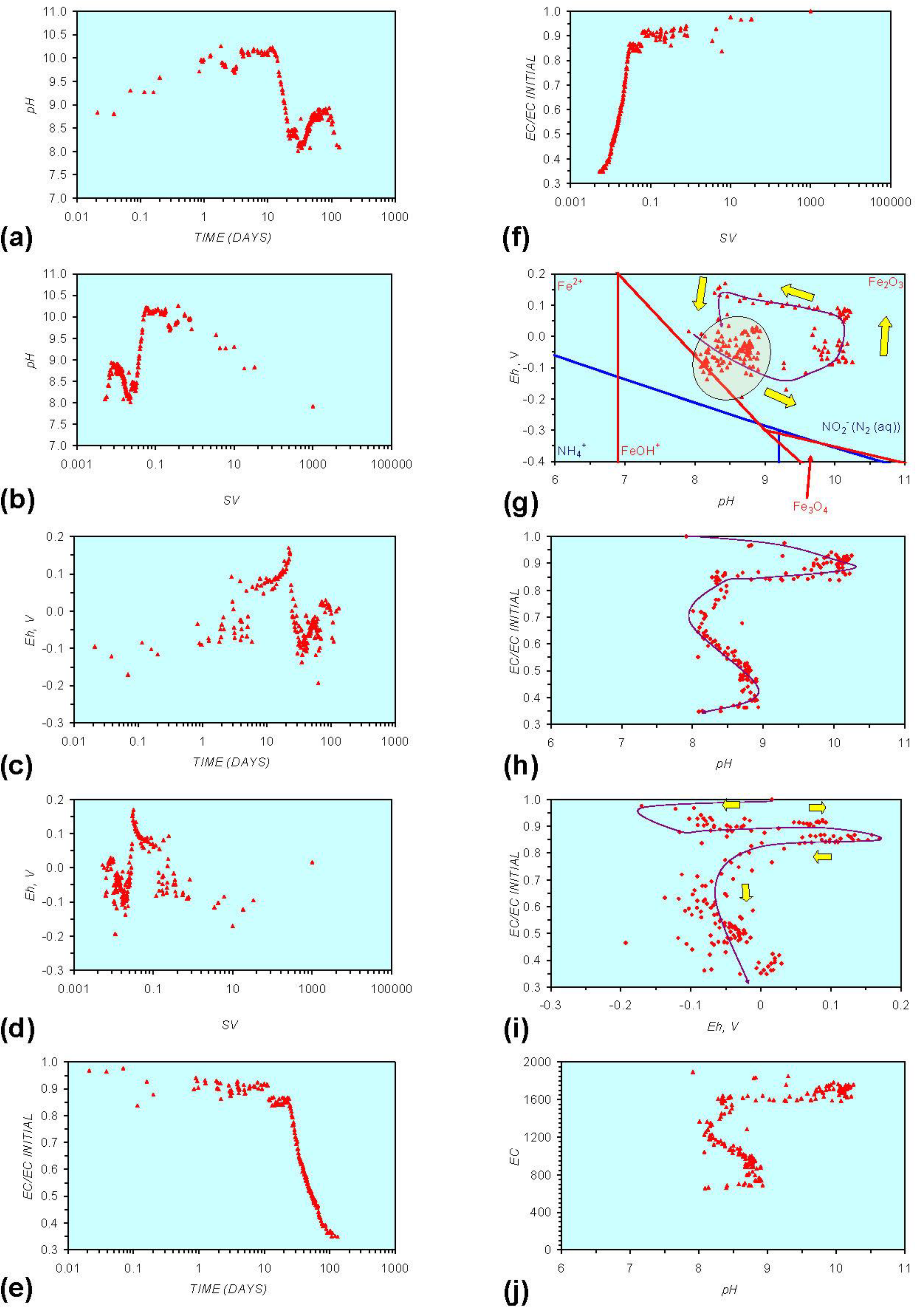
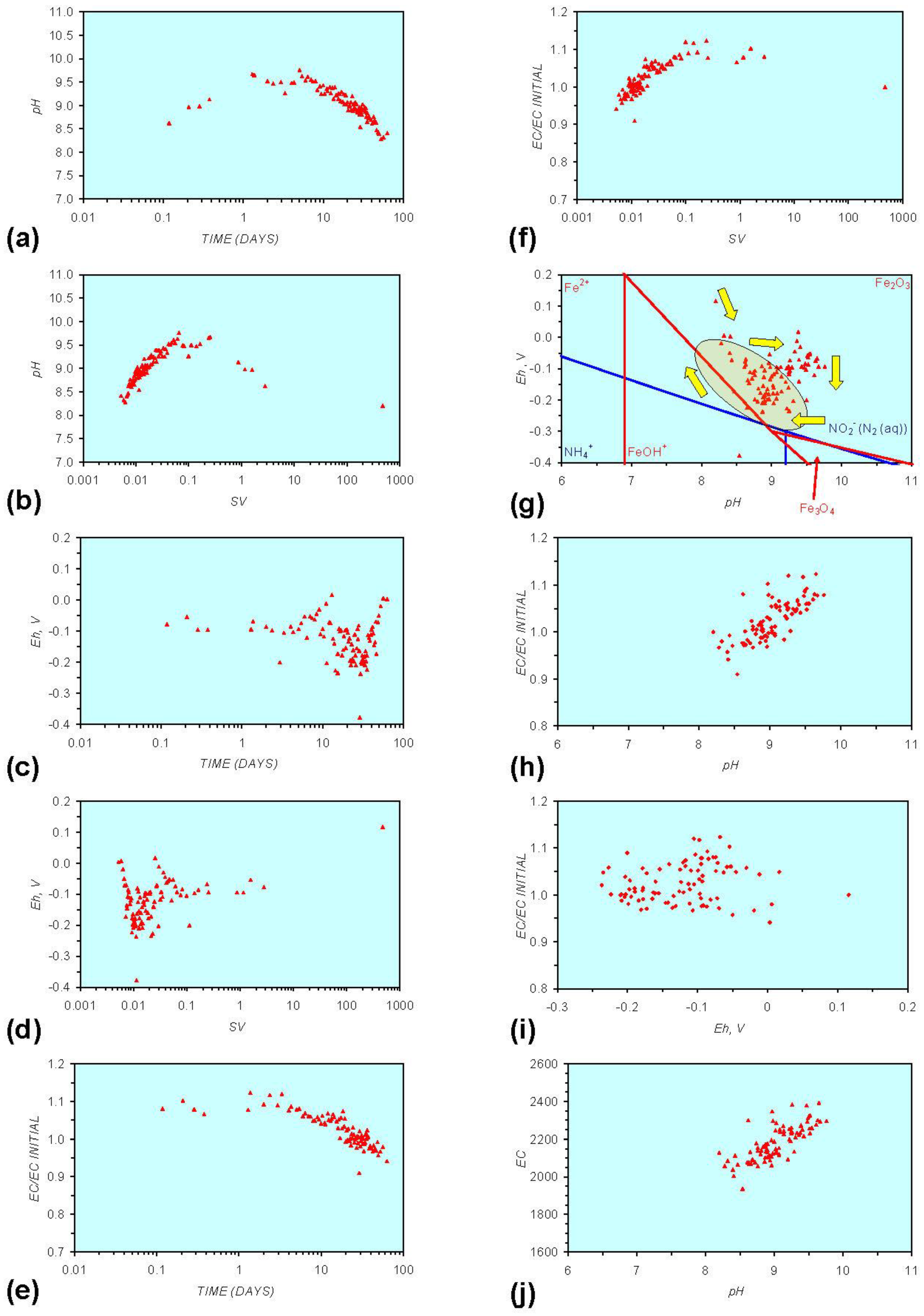
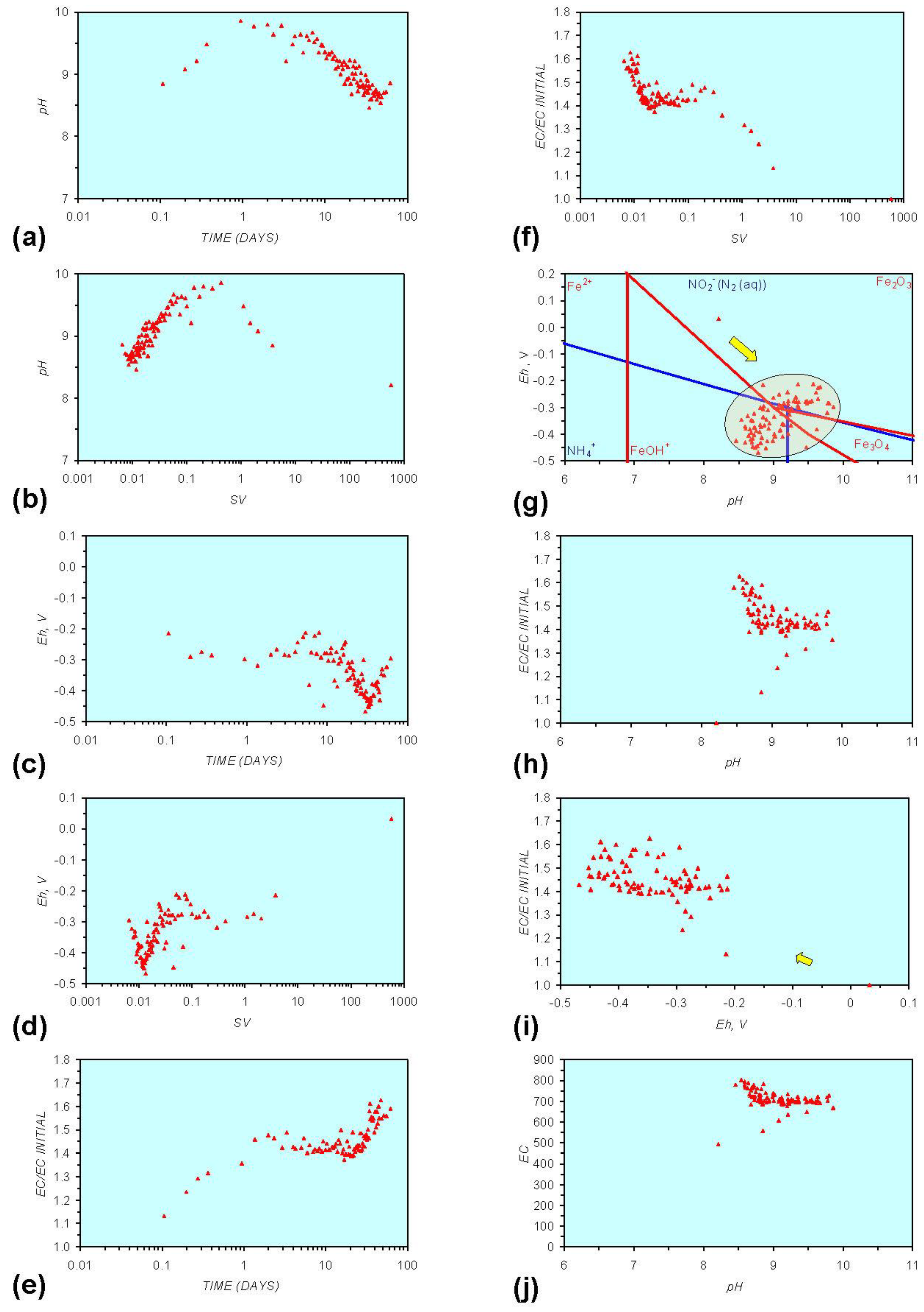
The addition of NaCl to the water appears to leave the Eh:pH location of the SRE unchanged (compare Figure A1g and Figure A7g in Appendix) When n-Fe0 + n-Cu0 + n-Al0 is present, the presence of NaCl initially results in the development of a common SRE at the end of the redox cycle (compare Figure A5g and Figure A8gin Appendix). However, in a saline environment, the Eh subsequently increases. This Eh increase is accompanied by a decrease in pH (Figure A8g in Appendix). This can result (Figure A8 in Appendix) in a similar starting and final Eh and pH.
When Ca-montmorillonite is present, the major decrease in Eh does not occur until the pH has reduced to its SRE level (Figure A10g, Figure A11g, Figure A13g, Figure A14g, Figure A15g and Figure A16g, in Appendix).
4. Interpretation
The test results (Figures A1–A16 in Appendix) have established that static diffusion associated with n-ZVM results in an Eh, pH, EC trajectory which can be related directly to time/space velocity. This trajectory is oscillatory, and its exact route varies with ZVM combinations and salinity.
4.1. Equilibrium Oscillation
Figures A1–A16 in Appendix demonstrate that Eh and pH is in a state of a perpetual equilibrium oscillation between reduction and oxidation reactions. For example, the reduction of Fe-OH (s) or Fe-OH (aq) (Equation 4)
oscillates with the oxidation of Fe0 or Fe-H+ (Equation 5)
zFeOH− + nH+ + mOqH− + kH2O + cFedOb = pFe0 + gFe-H+ + xH2O + yO2(g) + jOqH−
[O2 degassing, Eh reduction, and pH increase or decrease]
[O2 degassing, Eh reduction, and pH increase or decrease]
pFe0 + gFe-H+ + xH2O + rOqH− = cFedOb + zFeOH− + nH+ + mOqH− + hFe−H++ jH2(g)
[H+ ion or H2(g) formation, Eh and pH increase or decrease]
[H+ ion or H2(g) formation, Eh and pH increase or decrease]
yO2(g) can be present as H2O2 or as [H2O]m(O2)n. yH2(g) can be present as H3O+ or as [H2O]m(H2)n. Increases in Eh are associated with an increase in the HO2− (i.e., OH−[O]): OH− ratio [1]. Increases in pH result from a decrease in the H+:H2O ratio. The observed redox changes (Figures A1 to A16 in Appendix) can be linked directly to changes in these ion concentrations, and therefore to the redox reactions (Equations 3–8). Increases in EC are associated with aqueous ion formation (e.g., Fe2+, FeOH−) while the removal of aqueous ions is associated with a decrease in EC. Decreases in Eh, associated with increases in pH may be associated with the release of H2(g), but are commonly associated with the release of O2 resulting from the decomposition of H2O2.
The continual Eh:pH oscillation (Figures A1 to A16 in Appendix) interacts with ZVM to form nuclei of the generic form ZVM-(H+)n, ZVM-(O-H)n, ZVM-((CH)2)n, ZVM-CHn, ZVM-CHCl2, ZVM-CHCl3, ZVM-CHCl, and ZVM-CH2Cl [28,29,30,48]. These nuclei act as loci for organic matter remediation. Examples of ZVM nuclei formation are provided in Equation 6:
ZVM + H+ = ZVM-H+
ZVM-H+ + CO2 = ZVM-COOH+
ZVM-H+ + CO2 + xH+ = ZVM-CHn + 2H2O
ZVM-H+ + CH4 = ZVM-CH3 + 2H+
ZVM-H+ + CO2 + 6H+ = ZVM-CH3 + 2H2O
ZVM-H+ + CxH(2x+2) = ZVM-(CH2)(x-1)CH3 + 2H+
ZVM-H+ + CxHyCln = ZVM-CHCl or ZVM-CHCl2 or ZVM-CHCl3 or ZVM-CH2Cl
ZVM-H+ + CxHyOz + mH+ = ZVM-CpHq + nH2O
ZVM-H+ + CO2 = ZVM-COOH+
ZVM-H+ + CO2 + xH+ = ZVM-CHn + 2H2O
ZVM-H+ + CH4 = ZVM-CH3 + 2H+
ZVM-H+ + CO2 + 6H+ = ZVM-CH3 + 2H2O
ZVM-H+ + CxH(2x+2) = ZVM-(CH2)(x-1)CH3 + 2H+
ZVM-H+ + CxHyCln = ZVM-CHCl or ZVM-CHCl2 or ZVM-CHCl3 or ZVM-CH2Cl
ZVM-H+ + CxHyOz + mH+ = ZVM-CpHq + nH2O
4.2. Impact of CO2
Organic matter within an aquifer is degraded to form CO2 (aq) by biogenic activity [48]. Fe0 catalyses the formation of simple organic chains from the aqueous CO2 [1,49,50]. These form simple alkanes (methane, ethane, etc.) and simple oxygenates (e.g., acetone, butanone, methanal, ethanal, methanoic acid, ethanoic acid, etc.) [1,48]. These ZVM products replace the TCE’s, humic acids, dissolved organic matter, pesticides over a period of time [1,12,49,50]. The concentration of these products increases with time and may be directly linked to decreases in EC (e.g., Figure A6e in Appendix). These products may form a primary food source for the microbiota [48]. The general process of CO2 and halogen-alkane/alkene reutilisation to form, grow and release simple alkanes and alkenes is summarized in Equation 7 [1,48] as:
Fe0 + H2O = OH− + Fe-H+ − catalytic nuclei formation
Fe0 + H3O+ = Fe-H+ + H2O − catalytic nuclei formation
Fe-H+ + CO2 + 6H3O+ = Fe-CH3 + 8H2O − chain formation
Fe-CH3+ CO2 + 6H3O+ = Fe-CH2CH3 + 8H2O − chain growth
Fe-CH3+ CO2 + 6H3O+ = Fe-(CH2)2CH3 + 8H2O − chain growth
Fe-(CH2)2CH3 + 2H3O+ = Fe-H+ + 2H2O + CH3CH2CH3 − chain termination
ZVM + CxHyClz = ZVM-CaHbClc + … − catalytic nuclei formation
ZVM-CCl3 + CH4 = ZVM-CCl2CH3 + Cl− + H+ − chain growth
ZVM-CHCl2 + CH4 = ZVM-CH2CH3 + 2Cl− − chain growth
ZVM-CH2CH3 + CH4 = ZVM-CH2CH2CH3 + 2H+ − chain growth
ZVM-CHCl2 + 4H+ = ZVM-H+ + CH4 + 2Cl− − chain termination
ZVM-CH2CH2CH3 + 2H+ = ZVM-H+ + CH3CH2CH3 − chain termination
ZVM-CH2CH2CH3 + H+ = ZVM + CH3CH2CH3 − chain termination
ZVM-CH2CH3 + ZVM-CH2CH3 + 2H+ = 2ZVM-H+ + CH3 CH2CH2CH3 − chain termination
ZVM-CH2CH3 + ZVM-CH2CH3 = 2ZVM + CH3 CH2CH2CH3 − chain termination
CH4 can be replaced by CxHy or CxHyClz or CxHyOz [1]. The presence of CO2 in the water (from any source) results in a spontaneous interaction with Fe0 which can result (Equation 8) in the release of H2 [1,50,51].
CO2(g) = CO2 (aq) − ΔGo = +8.335 kJ mol−1
CO2(aq) + H2O (l) = HCO3−(aq) + H+ (aq) − ΔGo = +36.305 kJ mol−1
Fe0 + 2H+ (aq) = Fe2+ (aq) + H2(g) − ΔGo = −91.525 kJ mol−1
Fe0 + 2CO2(g) = 2HCO3− (aq) + Fe2+ (aq) + H2 (g) − ΔGo = −2.245 kJ mol−1
CO2(aq) + H2O (l) = HCO3−(aq) + H+ (aq) − ΔGo = +36.305 kJ mol−1
Fe0 + 2H+ (aq) = Fe2+ (aq) + H2(g) − ΔGo = −91.525 kJ mol−1
Fe0 + 2CO2(g) = 2HCO3− (aq) + Fe2+ (aq) + H2 (g) − ΔGo = −2.245 kJ mol−1
4.3. Fenton Reactions
Most aquifers are oxygenated to some extent, and most contain organic matter (OM). When Fe0 is added to water contaminated with organic matter (or containing Al cations or Al0) the first stage of the redox trajectory is a reduction in pH and Eh (Figures A1–A16 in Appendix) which is associated with O2 degassing (Figure A4, Figure A5 and Figure A6 in Appendix). This initial change is associated with Fenton reactions (Equation 9) [1,52,43]
O2 + Fe0 + 2H+ = H2O2 (aq) + Fe2+
OMoxidized 1 + Fe0 = OMreduced + Fe2+
OMreduced + O2 + 2H+ = H2O2 (aq) + OMoxidized 2
2H2O2 (aq) = 2H2O (l) + O2 (g)
2Fe0 + 2H2O = 2Fe-H+ + 2OH−
2Fe0 + O2 + 2H2O = 2Fe2+ + 4OH−
2Fe0 + 2H2O[O] = 2Fe2+ + 4OH−
2OH− = H2O2
Fe2++H2O2 = Fe3+ + 2OH−
OMoxidized 1 + Fe0 = OMreduced + Fe2+
OMreduced + O2 + 2H+ = H2O2 (aq) + OMoxidized 2
2H2O2 (aq) = 2H2O (l) + O2 (g)
2Fe0 + 2H2O = 2Fe-H+ + 2OH−
2Fe0 + O2 + 2H2O = 2Fe2+ + 4OH−
2Fe0 + 2H2O[O] = 2Fe2+ + 4OH−
2OH− = H2O2
Fe2++H2O2 = Fe3+ + 2OH−
O2 includes 2HO2− = 2OH− + O2. The ion concentrations (HCO3−, HO2−, OH−, Fen+, FeOH−) resulting from the interaction of Fe0 with CO2 (aq) and H2O vary as function of pore-water velocity and distance from the ZVM [53]. The primary reduction in DOM occurs after the pH has increased to a maximum value (Figure A6 in Appendix). This increase in pH is associated with a decrease in Eh (i.e., release of H+ (aq), removal of HO2− (aq).) and the formation of FeO(OH).nH2O at the ZVM—water interface, i.e., Fe0 + HO2− + nH2O = FeO(OH).nH2O.
4.4. Sulphur and Oxylate Removal
ZVM interacts with sulphur to form active sites [54] which can be used to remediate organic pollutants. These active sites take the form (Equation 10):
ZVM-H+ + aH2S (aq or g) = ZVM-Sa + (a+0.5)H2
ZVM-CH3+ H2S = CH3-ZVM-SH+ + 0.5H2
ZVM-CH3+ H2S = CH3-ZVM-SH+ + 0.5H2
Sulphur, like oxygen can be inserted into any C-C or C-H bond. Consequently, in sulphurous waters (or water containing sulphate fertilizer), ZVM treatment will result in the formation of ZVM-S, ZVM-OxS sites and associated CxHySn and CxHyNvSn compounds [54]. While the addition of H2S was not examined, it is a common biogenic product in many anoxic (low Eh) aquifers. The test results (Figures A1 to A16 in Appendix) establish that when Fe0 is present, the SRE, is anoxic (Eh < −0.1V) with an intermediate pH (8–10). In this environment biogenic activity will degrade sulphur compounds (e.g., SO42−) to H2S and will produce oxylates. The ZVM will reduce this H2S to form active sites with the associated formation of H+, H2(g), H3O+, H2O[H2]n, and ZVM-H+. The FeS-H2S/FeS2 redox couple can be linked to CO2 reduction [55], where 2FeS + 2CO2 [or + H2C2O4] + 2H2O = FeS2 + Fe-C2O4.2H2O [or Fe-C2O4.2H2O + H2] [56]. These observations indicate that ZVM treatment of sulphur rich waters (with a low throughflow) containing organic contaminants, will result in organic decontamination, CO2 removal, and removal of sulphur from the aquifer. Electrochemical ZVM-oxylate formation is induced by reducing Eh [57]. Reductions of >−0.03 V are required [57]. Figures A1–A16 in Appendix demonstrate Eh reductions of −0.2 to >−0.5. This indicates that ZVM-oxylate formation will occur in the SRE and along the redox trajectory when the porewater contains one or more of H2C2O4, HC2O4−, and C2O42−. The principal Fe sites formed by this process include FeC2O4+, Fe(C2O4)2− , Fe(C2O4)33− and FeHC2O42+ [58].
4.5. General Patterns
The interaction between reductive and oxidative reactions results in the development of a SRE (e.g., Figure A1g in Appendix). The interaction is complex and involves all organic and metal species contained within the water and associated matrix (e.g., clays). Consequently, within aquifers involving a large number of species there will be a high variance on Eh, pH with time or SV. This will be associated with sequential oscillations between progressive reductive and oxidative states. However, Figure A5, Figure A6, Figure A11 and Figure A16, in Appendix demonstrate that as the number of active ZVM site types increase, the Eh, pH and EC variance associated with a specific SV decreases. Figure A6 demonstrates that these active sites can be organic and can be in solution (e.g., DOM). Specific observations in a simple ZVM-water system are:
- (i)
- (ii)
- The formation of Al3+ (aq) ions, resulting in a substantial increase in EC (Figure A2 in Appendix) is linked directly to a decrease in Eh and an increase in pH, e.g., H+ + HO2− = 2OH− (or H2O2).
In both examples, the major formation of metal ions (aq) can be avoided by maintaining a high space velocity through the aquifer. The addition of a second zero valent metal (Figure A3, Figure A4 and Figure A5) or organic material (Figure A6 in Appendix) or NaCl (Figure A7, Figure A8, Figure A13, Figure A14, Figure A15, and Figure A16 in Appendix prevents the formation of substantial quantities of FeOH− (aq) (Figures A1 and A10 in Appendix) and accelerates the reduction in EC (i.e., removal of dissolved material). In this instance the major removal of pollutants occurs 10–200 days after the ZVM is placed in the aquifer (Figure A3, Figure A4 and Figure A5 in Appendix).
In aquifers containing Ca-montmorillonite the change in redox environment associated with the SRE is associated with a net desalination of the aquifer [1]. The degree of desalination increases with decreasing SV. The desalination is associated with substitution of Ca cations with Na cations in the montmorillonite. At low SV in Figure A13, Figure A14, Figure A15 and Figure A16 in Appendix, the SRE is associated with an Eh within the range −0.1 to −0.5 V. This indicates that cation exchange is also associated with the removal of HO2−, or an increase in OH−. The latter may result from the removal of Ca hydration shells within the clay, as part of the cation substitution process.
4.6. Removal of Dissolved Organic Matter
Humic acids (HA) are complex structures containing phenolic and carboxylic groups. They have the ability to form complexes (including chelates) with Fe, Ca, Mg, K and other aqueous metal ions. Dissolved organic matter (e.g., Humic acids) have been demonstrated to shorten the effective operating life of n-Fe0 for the removal of dissolved Zn and Ni species, but not Cr species [59]. The removal of Zn (aq) species (by oxide formation) increases with increasing pH [60], while the removal of Ni (aq) species decreases with increasing Eh [60]. Cr removal occurs when the pH increases above 3 when Eh is between 0.9 and −0.5 [60]. This study has demonstrated that DOM is removed by ZVM (Figure A6 in Appendix) and that initial increases in pH and decreases in Eh are followed by a cycle of increasing Eh, decreasing pH and decreasing Eh. It has also been demonstrated that as m-ZVM loses its ability (due to oxide formation) to remediate water its pH decreases and Eh increases [1].
While this study has demonstrated removal from low surface area n-ZVM (Table 1), most academic studies focus on high surface area (e.g., 24–32 m2 g−1) n-Fe0 [61]. These studies have demonstrated that
- a)
- the rate HA removal increases with increasing n-Fe0 concentration (though k remains constant) [61], indicating that the removal may be linked to surface area.
- b)
- HA removal is associated with a significant decrease in pH [61].
- c)
- HA removal is associated over time with a change in n-Fe0 elemental ratio (Fe:O:C) from 85:13.5:0 (at onset) to 31:52:17 (after 90 days) [61].
This study has demonstrated (Figure A6) that significant DOM removal only occurs when the Eh starts to decrease as the water redox environment moves into the SRE. The Fe0 was oxidized at the water ZVM interface (to form iron hydroxides), but remained as reduced n-Fe0 below the interface zone. Dechlorination studies of tetrachloroethylene using palladized n-Fe0 have demonstrated that the rate of dechlorination to ethane and ethylene is increased by increasing the concentration of HA [62]. This indicates that HA may act as electron shuttles [62]. However, different types of DOM/HA may interact differently with nanoparticles and electrolytes [63].
The experimental results (Figure A6 in Appendix) suggest that Fe0 may act as an electron shuttle (catalyst) whereby organic acids mediate electron transfer to O2 [HO2−, H2O2] resulting in the formation of OH radical–mediated oxidation of organic compounds through the Fenton Reaction [1,51]. The electron shuttle reaction can be simplified [1] (Equation 11) to:
Fe0 + 2H2O = 2OH− + Fe-H2 = Fe2+ + 4H+ + O2(g)
This electron shuttle process decreases Eh (by production of OH−) and subsequent decreases in pH (associated with the co-release of H+ and O2) are prevented by capture of H+ in organic chain formation/breaking reactions. O2 release is associated with the formation of negative Eh and Eh declines are associated with the release of Fe ions [1].
Organic matter (e.g., pyridinium) can act as an electron shuttle to catalyse the reduction of CO2 to carboxylic acids, aldehydes and alcohols [64]. DOM (HA) can enhance Fe(II) and Fe(III) oxide reduction by both electron shuttling and Fe(II) complexation [65,66]. Reduced HA will reductively transform chlorinated solvents and nitroaromatic [66].
The presence of organic matter (and microbial activity) in an aquifer can therefore be expected to complicate the overall remediation process, particularly when the n-ZVM has a high surface area [66]. In this environment, the DOM/HA may foul the n-ZVM [61]. This study has established (compare Figures A1 and Figures A6 in Appendix) that when the n-ZVM has a low surface area (Table 1), the primary control on remediation shifts from n-ZVM surface area dependent interactions (e.g., adsorption/desorption reactions) to electrochemical reactions associated with H+, OH− and HO2− ion concentrations in the aquifer. Many of these reactions have negative activation energies and high rate constants at the aquifer temperature [38,39]. This results in a direct relationship between the level of remediation (EC reduction), Eh, pH and n-ZVM concentration.
These observations suggest that switching n-ZVM remedial programs from the use of high cost, high surface area n-ZVM (derived from Fe ion precipitation) to the substantially lower cost, low surface area n-ZVM (derived from ground metals) may have significant benefits for a IZVM or PRB remediation program. These benefits include:
- a)
- Reduced cost. n-ZVM (n-ZVMA) derived from a ground metal is typically about 10% of the cost of n-ZVM (n-ZVMB) produced by precipitation from a nitrate, chloride or sulphate.
- b)
- Increased active life. n-ZVMA is less prone to fouling by DOM/HA than n-ZVMB [61].
- c)
- Increased activity. n-ZVMA produces larger shifts in both pH and Eh than n-ZVMB (Figures A1–A16) or m-ZVM [1].
- d)
- Increased control on product selectivity. Figures A1 to A16 in Appendix demonstrate that changing the concentrations of ZVM components can alter the redox trajectory, Eh, pH and consequently the degree and level of remediation. The use of ground metal particles, rather than bi-metal or tri-metal precipitated complexes, allows the relative ratios of Fe:Cu:Al to be rapidly adjusted during the course of the remediation program in order to compensate for redox changes/interactions associated with the aquifer microbiota, aquifer chemistry, interactions with the host rock minerals and changes in the aquifer flow rate.
5. Conclusions
This study has established that there is a common Eh-pH trajectory with time and space velocity for Fe0, when added to water. This trajectory is modified by the presence of Cu0, or Al0, or NaCl, or clay, but is unaffected by the presence of dissolved organic matter. The Eh-pH environment in the aquifer can be predicted from the regression relationships encapsulated by the graphs of Eh and pH vs. SV in the Appendix. In these relationships SV is directly related to a target aquifers pore volume, the amount of ZVM injected, the throughflow rate in the aquifer, changing aquifer permeability and time.
Aquifer remediation is a function of individual equilibrium redox reactions, the product of the constant oscillation between reduction and oxidation and the catalytic reformation CxHy, CxHyOz and COx to simple organic compounds which can be removed by the microbiota. The establishment of a redox trajectory which is linked directly to SV, allows ZVM aquifer remediation programs to be designed to target a specific redox environment with a specific timeframe. This remediation approach has already been shown to be effective for m-ZVM [1]. This study demonstrates that a similar approach could be applied to n-ZVM associated with IZVM and PRB programs.
Static diffusion affects water flowing through IZVM and PRB’s, and provides a halo of remediation around the n-ZVM zone. This study has demonstrated (i) that n-ZVM can be used to provide similar levels of treatment for both saline and freshwater, (ii) that the presence of clays can be used to reinforce treatment trajectories. In a previous study [1], it was observed that placement of m-ZVM in a PRB provided a less effective aquifer treatment than recirculation through a continuous flow reactor. The redox trajectories (Figures A1–A16) associated with n-ZVM have a lower variance than the similar trajectories associated with m-ZVM. This difference has significant implications for PRB design, particularly in impermeable or low permeability sediments. Static groundwater mounds are common in low permeability sediments [24,25,26,27]. When surface water runoff is directed to infiltration devices in impermeable/low permeability sediments, the infiltration devices will frequently contain static (standing) water between recharge events [24,25,26,27]. The air-water contact represents the upper surface of a perched (self-sealing) ground water mound which extends spatially into the surrounding sediment [24,25,26,27]. Consequently, placement of n-ZVM in the infiltration devices below the air-water contact will allow modification of the Eh and pH of the static ground water mound by static diffusion. This allows placement of PRB’s in infiltration devices to provide targeted pollutant removal from overland flow (associated with sustainable urban drainage schemes (SUDS)), and a targeted reconstruction of the redox environment of the associated perched groundwater mounds [25,26,27].
Acknowledgements
The two reviewers are thanked for their helpful and constructive comments on an earlier draft.
References
- Antia, D.D.J. Sustainable zero-valent metal (ZVM) water treatment associated with diffusion, infiltration, abstraction and recirculation. Sustainability 2010, 2, 2988–3073. [Google Scholar] [CrossRef]
- Chuang, F-W.; Larson, R.A.; Wessman, M.S. Zero-valent iron-promoted dechlorination of polychlorinated biphenyls. Environ. Sci. Technol. 1995, 29, 2460–2463. [Google Scholar]
- Orth, R.; Daudo, T.; McKenzie, D.E. Reductive dechlorination of DNAPL Trichloroethylene by zero-valent iron. Prac. Period. Hazard. Toxic. Radioact. Waste Manag. 1998, 2, 123–128. [Google Scholar] [CrossRef]
- Chen, J.L.; Al-Abed, S.R.; Ryan, J.A.; Li, Z. Effects of pH on dechlorination of trichloroethylene by zero-valent iron. J. Hazard Mater. 2001, 83, 243–254. [Google Scholar] [CrossRef] [PubMed]
- Lowry, G.V.; Johnson, K.M. Congener-specific dechlorination of dissolved PCBs by microscale and nanoscale zerovalent iron in water/methanol solution. Environ. Sci. Technol. 2004, 38, 5208–5216. [Google Scholar] [CrossRef] [PubMed]
- Shin, M-C.; Choi, H-D.; Kim, D-H.; Baek, K. Effect of surfactant on reductive dechlorination of trichloroethylene by zero-valent iron. Desalination 2008, 223, 299–307. [Google Scholar]
- Kim, G.; Jeong, W.; Choe, S. Dechlorination of atrazine using zero-valent iron (Fe0) under neutral pH conditions. J. Hazard. Mater. 2008, 155, 502–506. [Google Scholar] [CrossRef] [PubMed]
- Ghazali, M.; McBean, E.; Shen, H.; Dastous, P-A. Impact of iron concentration and ph on zero-valent iron dechlorination of DDT for brownfields. Remediat. J. 2010, 20, 97–107. [Google Scholar] [CrossRef]
- Thompson, J.M.; Chisholm, B.J.; Bezbaruah, A.N. Reductive dechlorination of Chloroactetanilide herbicide (Alachlor) using zero-valent iron nanoparticles. Environ. Engrg. Sci. 2010, 27, 227–232. [Google Scholar] [CrossRef]
- McElroy, B.; Keith, A.; Glasgow, J.; Dasappa, S. The use of zero-valent iron injection to remediate groundwater: Results of a pilot test at Marshall space flight center. Remediation 2003, 13, 145–153. [Google Scholar] [CrossRef]
- Demonstration of in situ Dehalogenation of DNAPL through Injection of Emulsified Zero-Valent Iron at Launch Complex 34 in Cape Canaveral Air Force Station, Florida; Innovative Technology Evaluation Report, EPA/540/R-07/006; U.S. Environmental Protection Agency: Cincinnati, OH, USA, September 2004.
- Gavaskar, A.; Tatar, L.; Condit, W. Cost and Performance Report: Nanoscale Zero-Valent Iron Technologies for Source Remediation; Contract Report CR-05-007-ENV; Naval Facilities Engineering Command/Engineering Service Center (NAVFAC ESC): Port Hueneme, CA, USA, 2005; p. 44. [Google Scholar]
- Pupeza, M.; Cernik, M.; Greco, M. Dechlorination of chlorinated hydrocarbons by zero-valent iron nano-particles. NATO Sci. Ser. 2007, 75, 111–118. [Google Scholar]
- Gavaskar, A.; Bhargava, M.; Condit, W. Cost and Performance Report for a Zero-Valent Iron (ZVI) Treatability Study at Naval Air Station North Island; Technical Report TR-2307-ENV; Naval Facilities Engineering Command/Engineering Service Center (NAVFAC ESC): Port Hueneme, CA, USA, 2008. [Google Scholar]
- Alvarado, J.S.; Rose, C.; LaFreniere, L. Degradation of carbon tetrachloride in the presence of zero-valent iron. J. Environ. Monit. 2010, 12, 1524–1530. [Google Scholar] [CrossRef] [PubMed]
- Sunkara, B.; Zhan, J.; He, J.; McPherson, G.L.; Piringer, G.; John, V.T. Nanoscale zerovalent iron supported on uniform carbon microspheres for the in situ remediation of chlorinated hydrocarbons. ACS Appl. Mater. Interfaces, 2010, 2, 285–2862. [Google Scholar] [CrossRef]
- Sorel, D.; Warner, S.D.; Longino, B.L.; Honniball, J.H.; Hamilton, L.A. Performance monitoring and dissolved hydrogen measurements at a permeable zero valent iron reactive barrier. ACS Symp. Ser. 2002, 837, 278–285. [Google Scholar]
- Choi, J-H.; Kim, Y-H.; Choi, S.J. Reductive dechlorination and bidegradation of 2,4,6-trichlorophenol using sequential permeable reactive barriers: laboratory studies. Chemosphere 2007, 67, 1551–1557. [Google Scholar] [CrossRef] [PubMed]
- Sass, B.M. Reduction of TNT and RDX by core material from an iron permeable reactive barrier. Paper M-009. In Proceedings of the 6th International Conference on Remediation of Chlorinated and Recalcitrant Compounds, Monterey, CA, USA, May 2008; Battelle: Columbus, OH, USA, 2008. [Google Scholar]
- Higgins, M.R.; Olson, T.M. Life-cycle case study comparison of permeable reactive barrier versus pump-and-treat remediation. Environ. Sci. Technol. 2009, 43, 9432–9438. [Google Scholar] [CrossRef] [PubMed]
- Phillips, D.H.; Van Nooten, T.; Bastiaens, L.; Russell, M.I.; Dickson, K.; Plant, S.; Ahad, J.M.; Newton, T.; Elliot, T.; Kalin, R.M. Ten year performance evaluation of a field-scale zero-valent iron permeable reactive barrier installed to remediate trichloroethene contaminated groundwater. Environ. Sci. Technol. 2010, 15, 3861–3869. [Google Scholar] [CrossRef]
- Gilbert, O.; de Pablo, J.; Cortina, J.-L.; Ayora, C. In situ removal of arsenic from groundwater by using permeable reactive barriers of organic matter/limestone/zero-valent iron mixtures. Environ. Geochem. Health 2010, 32, 373–378. [Google Scholar] [CrossRef] [PubMed] [Green Version]
- Luo, H.; Jin, S.; Fallgren, P.H.; Colberg, P.J.S.; Johnson, P.A. Prevention of iron passivation and enhancement of nitrate reduction by electron supplementation. Chem. Eng. J. 2010, 160, 185–189. [Google Scholar] [CrossRef]
- Antia, D.D.J. Prediction of overland flow and seepage zones associated with the interaction of multiple Infiltration Devices (Cascading Infiltration Devices). Hydrol. Proc. 2008, 22, 2595–2614. [Google Scholar] [CrossRef]
- Antia, D.D.J. Formation and control of self-sealing high permeability groundwater mounds implications for SUDS and sustainable pressure mound management. Sustainability 2009, 1, 855–923. [Google Scholar] [CrossRef]
- Antia, D.D.J. Interacting Infiltration Devices (Field Analysis, Experimental Observation and Numerical Modeling): Prediction of Seepage (Overland Flow) Locations, Mechanisms and Volumes–Implications for SUDS, Groundwater Raising Projects. In Hydraulic Engineering: Structural Applications, Numerical Modeling and Environmental Impacts, 1st ed.; Hirsch, G., Kappel, B., Eds.; Nova Science Publishers: Hauppauge, NY, USA, 2010; pp. 85–156. [Google Scholar]
- Antia, D.D.J. Interpretation of Overland Flow Associated with Infiltration Devices Placed in Boulder Clay and Construction Fill. In Overland Flow and Surface Runoff, 1st ed.; Wong, T.S.W., Ed.; Nova Science Publishers: Hauppauge, NY, USA, 2011. (In Press) [Google Scholar]
- Fiore, S.; Zanetti, M.C. Preliminary tests concerning zero-valent iron efficiency in organic pollutants removal. Am. J. Environ. Sci. 2009, 5, 555–560. [Google Scholar] [CrossRef]
- Hao, Z.W.; Xu, X.H.; Wang, D.H. Reductive denitrification of nitrate by scrap iron filings. J. Zhejang Univ. Sci. B. 2005, 6, 182–186. [Google Scholar] [CrossRef]
- Hao, Z.W.; Xu, X.H.; Jin, J.; He, P.; Liu, Y.; Wang, D.H. Simultaneous removal of nitrate and heavy metals by iron metal. J. Zhejang Univ. Sci. B. 2005, 6, 307–310. [Google Scholar] [CrossRef]
- Zhang, W-X. Nanoscale iron particles for environmental remediation: An overview. J. Nanoparticle Res. 2003, 5, 323–332. [Google Scholar]
- Wang, C-B.; Zhang, W-X. Synthesising nano-scale iron particles for rapid and complete dechlorination of TCE and PCBs. Environ. Sci. Technol. 1997, 31, 2154–2156. [Google Scholar]
- Liu, Y.; Majetich, S.A.; Tilton, R.D.; Sholl, D.S.; Lowry, G.V. TCE dechlorination rtaes, pathways and efficiency of nanoscale particles with different properties. Environ. Sci. Technol. 2005, 39, 1338–1345. [Google Scholar] [CrossRef] [PubMed]
- Tokoro, H.; Nakabayashi, T.; Fujii, S.; Zhao, H.; Hafeli, U.O. Magnetic iron particles with high magnetization useful for immunoassay. J. Magnetism Magnetic Mat. 2009, 321, 1676–1678. [Google Scholar] [CrossRef]
- Antony, J.; Nutting, J.; Baer, D.R.; Meyer, D.; Sharma, A.; Qiang, Y. Size-dependent specific surface area of nanoporous film assembled by core-shell iron nanoclusters. J. Nanomat. 2006, 1, 1–4. [Google Scholar] [CrossRef]
- Krasnoperov, L.N.; Peng, J.; Marshall, P. Modified transition state theory and negative apparent activation energies of simple metathesis reactions: Application to the reaction CH3 + HBr = CH4 + Br. J. Phys. Chem. A 2006, 110, 3110–3120. [Google Scholar] [CrossRef] [PubMed]
- Wei, J. Adsorption and cracking of n-alkanes over ZSM-5: negative activation energy of reaction. Chem. Engrg. Sci. 1996, 51, 2995–2999. [Google Scholar] [CrossRef]
- Alvarez-Idaboy, J.R.; Mora-Diez, N.; Vivier-Bunge, A. A quantum chemical and classical transition state theory explanation of negative activation energies in OH addition to substituted ethenes. J. Am. Chem. Soc. 2000, 122, 3715–3720. [Google Scholar] [CrossRef]
- Alvarez-Idaboy, J.R.; Mora-Diez, N.; Boyd, R.J.; Vivier-Bunge, A. On the importance of prereactive complexes in molecule-radical reactions: hydrogen abstraction from aldehydes by OH. J. Am. Chem. Soc. 2001, 123, 2018–2024. [Google Scholar] [CrossRef] [PubMed]
- Cunningham, D.A.H.; Vogel, W.; Haruta, M. Negative activation energies in CO oxidation over an icosahedral Au/Mg(OH)2 catalyst. Cat. Let. 1999, 63, 43–47. [Google Scholar] [CrossRef]
- Brookhaven National Laboratory Carbon Dioxide (Reduction); Report BNL-67077(Produced for the U.S. Department of Energy), Contract DE-AC02-98CH10886; Brookhaven National Laboratory: Long Island, NY, USA, 1998; p. 10.
- Perkins, H.F.; Parker, M.B.; Walker, M.L. Chicken Manure—Its Production, Composition and Use as a Fertilizer; Georgia Agricultural Experiment Stations, University of Georgia College of Agriculture: Athens, GA, USA, 1964. [Google Scholar]
- Dikinya, O.; Mufwanzala, N. Chicken manure—enhanced soil fertility and productivity: Effects of application rates. J. Soil Sci. Environ. Manag. 2010, 1, 46–54. [Google Scholar]
- Materechera, S.A.; Mkhabela, T.S. The effectiveness of lime, chicken manure and leaf litter ash in ameliorating acidity in a soil previously under black wattle (Acacia mearnsii) plantation. Biores. Technol. 2002, 85, 9–16. [Google Scholar] [CrossRef]
- Himathongkham, S.; Bahari, S.; Riemann, H.; Cliver, D. Survivial of Escherichia coli O157:H7 and Salmonella typhimurium in cow manure and cow slurry. FEMS Mircobiol. Let. 1999, 178, 251–257. [Google Scholar] [CrossRef]
- Kunz, A.; Steinmetz, R.L.R; Ramme, M.A.A.; Coldebella, A. Effect of storage time on swine manure solid separation by screening. Biores. Technol. 2009, 100, 1815–1818. [Google Scholar] [CrossRef]
- Xing, Y.; Li, Z.; Fan, Y.; Hou, H. Biohydrogen production from dairy manures with acidification pretreatment by anaerobic fermentation. Environ. Sci. Pollut. Res. Int. 2010, 17, 392–399. [Google Scholar] [CrossRef] [PubMed]
- Antia, D.D.J. Oil polymerisation and fluid expulsion from low temperature, low maturity, over pressured sediments. J. Petrol. Geol. 2008, 31, 263–282. [Google Scholar] [CrossRef]
- Elek, J. Homogenous Catalytic Reduction of CO2 in Aqueous Medium. PhD Thesis, University of Debrecen, Debrecen, Hajdu-Bihar, Hungary, 2003. [Google Scholar]
- Guan, G.; Kida, T.; Ma, T.; Kimura, K.; Abe, E.; Yoshida, A. Reduction of aqueous CO2 at ambient temperature using zero-valent iron-based composites. Green Chemistry 2003, 5, 630–634. [Google Scholar] [CrossRef]
- Kang, S.H.; Choi, W. Oxidative degradation of organic compounds using zero-valent iron in the presence of natural organic matter serving as an electron shuttle. Environ. Sci. Technol. 2009, 43, 878–883. [Google Scholar] [CrossRef] [PubMed]
- Rahmani, A.R.; Zarrabi, M.; Samarghandi, M.R.; Afkhami, A.; Ghaffari, H.R. Degradation of Azo Dye Reactive Black 5 and Acid Orange 7 by Fenton like mechanim. Iranian J. Chem. Eng. 2010, 7, 87–94. [Google Scholar]
- Wang, F. Modelling of Aqueous Carbon Dioxide Corrosion in Turbulent Pipe Flow. PhD Thesis, University of Saskatchewan, Saskatoon, Canada, 1999. [Google Scholar]
- Schmitt-Kopplin, P.; Gabelica, Z.; Gougeon, R.D.; Fekete, A.; Kanawati, B.; Harir, M.; Gebefugi, I.; Eckel, G.; Hertkorn, N. High molecular diversity of extraterrestrial organic matter in Murchison meteorite revealed 40 years after its fall. PNAS 2010, 107, 2763–2768. [Google Scholar] [CrossRef] [PubMed]
- Drobner, E.; Huber, H.; Wachterhauser, G.; Rose, D.; Stetter, K.O. Pyrite formation linked with hydrogen evolution under anaerobic conditions. Nature 1990, 346, 742–744. [Google Scholar] [CrossRef] [Green Version]
- Chai, L.; Navrotsky, A. Enthalpy of formation of siderite and its application in phase equilibria calculation. Am. Mineral. 1994, 79, 921–929. [Google Scholar]
- Angamuthi, R.; Byers, P.; Lutz, M.; Spek, A.L.; Bouwman, E. Electrocatalytic CO2 conversion to oxylate by a copper complex. Science 2010, 327, 313–315. [Google Scholar] [CrossRef] [PubMed]
- Baur, R.F.; Smith, W.M. The mono-oxalato complexes of iron (III). Can. J. Chem. 1965, 43, 2755–2762. [Google Scholar] [CrossRef]
- Dries, J.; Bastiaens, L.; Springael, D.; Kuypers, S.; Agathos, S.N.; Diels, L. Effect of humic acids on heavy metal removal by zero-valent iron in batch and continuous flow column systems. Water Res. 2005, 39, 3531–3540. [Google Scholar] [CrossRef] [PubMed]
- Geological Survey Japan. Atlas of Eh-pH Diagrams; Open File Report No. 419; National Institute of Advanced Industrial Science and Technology: Naoto, Japan, 2005.
- Giasuddin, A.B.M.; Kanel, S.R.; Choi, H. Adsorption of humic acid onto nanoscale zerovalent iron and its effect on arsenic removal. Environ. Sci. Technol. 2007, 41, 2022–2027. [Google Scholar] [CrossRef] [PubMed]
- Doong, R-A.; Lai, Y-J. Dechlorination of tetrachloroethylene by palladized iron in the presence of humic acid. Water Res. 2005, 39, 2309–2318. [Google Scholar]
- Liu, X.; Wazne, M.; Han, Y.; Christodoulatos, C.; Jasinkiewicz, K.L. Effects of natural organic matter on aggregation kinetics of boron nanoparticles in monovalent and divalent electrolytes. J. Colloid. Interface Sci. 2010, 348, 101–107. [Google Scholar] [CrossRef] [PubMed]
- Cole, E.B.; Lakkaraju, P.S.; Rampulla, D.M.; Morris, A.J.; Abelev, E.; Bocarsly, A.B. Using a one-electron shuttle for the multielectron reduction of CO2 to methanol: Kinetic, mechanistic and structural insights. J. Am. Chem. Soc. 2010, 132, 11539–11551. [Google Scholar] [CrossRef] [PubMed]
- Royer, R.A.; Burgos, W.D.; Fischer, A.S.; Unz, R.F.; Dempsey, B.A. Enhancement of biological reduction of hematite by electron shuttling and Fe(II) complexation. Environ. Sci. Technol. 2002, 36, 1939–1946. [Google Scholar] [CrossRef] [PubMed]
- Kappler, A.; Benz, M.; Schink, B.; Brune, A. Electron shuttling via humic acids in microbial iron (III) reduction in a freshwater sediment. FEMS Microbiol. Ecol. 2004, 47, 85–92. [Google Scholar] [CrossRef] [PubMed]
Appendix
The experimental results for n-ZVM are provided in Figures A1 to A16. EC = μS cm−1. Eh = V.
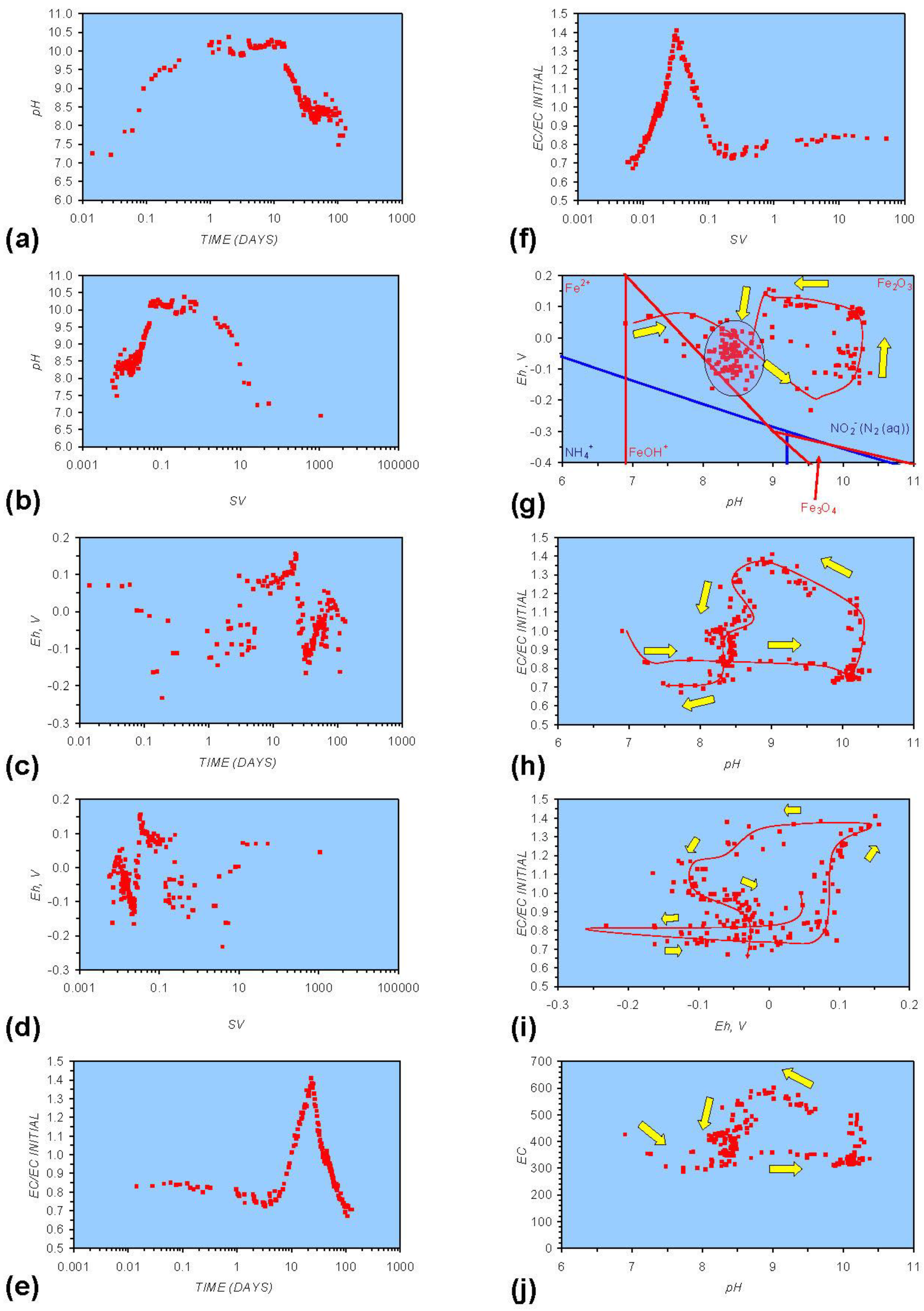
Figure A1.
MR1: n-Fe0, fresh water. (a) pH vs. Time; (b) pH vs. SV; (c) Eh vs. time; (d) Eh vs. SV; (e) EC/EC Initial vs. time; (f) EC/EC Initial vs. SV; (g) Eh vs. pH (SRE ringed); (h) pH vs. EC/EC Initial; (i) Eh vs. EC/EC Initial; (j) pH vs. E(C) Arrows indicate decreasing SV and increasing tim(e).

Figure A2.
MR2: n-Al0, fresh water. (a) pH vs. Time; (b) pH vs. SV; (c) Eh vs. time; (d) Eh vs. SV; (e) EC/EC Initial vs. time; (f) EC/EC Initial vs. SV; (g) Eh vs. pH (SRE ringed); (h) pH vs. EC/EC Initial; (i) Eh vs. EC/EC Initial; (j) pH vs. E(C) Arrows indicate decreasing SV and increasing tim(e).

Figure A3.
MR3: n-Fe0 + n-Cu0, fresh water. (a) pH vs. Time; (b) pH vs. SV; (c) Eh vs. time; (d) Eh vs. SV; (e) EC/EC Initial vs. time; (f) EC/EC Initial vs. SV; (g) Eh vs. pH (SRE ringed); (h) pH vs. EC/EC Initial; (i) Eh vs. EC/EC Initial; (j) pH vs. E(C) Arrows indicate decreasing SV and increasing tim(e).

Figure A4.
MR4: n-Fe0 + n-Al0, fresh water. (a) pH vs. Time; (b) pH vs. SV; (c) Eh vs. time; (d) Eh vs. SV; (e) EC/EC Initial vs. time; (f) EC/EC Initial vs. SV; (g) Eh vs. pH (SRE ringed); (h) pH vs. EC/EC Initial; (i) Eh vs. EC/EC Initial; (j) pH vs. E(C) Arrows indicate decreasing SV and increasing tim(e).

Figure A5.
MR5: n-Fe0 + n-Al0 + n-Cu0, fresh water. (a) pH vs. Time; (b) pH vs. SV; (c) Eh vs. time; (d) Eh vs. SV; (e) EC/EC Initial vs. time; (f) EC/EC Initial vs. SV; (g) Eh vs. pH (SRE ringed); (h) pH vs. EC/EC Initial; (i) Eh vs. EC/EC Initial; (j) pH vs. E(C) Arrows indicate decreasing SV and increasing tim(e).

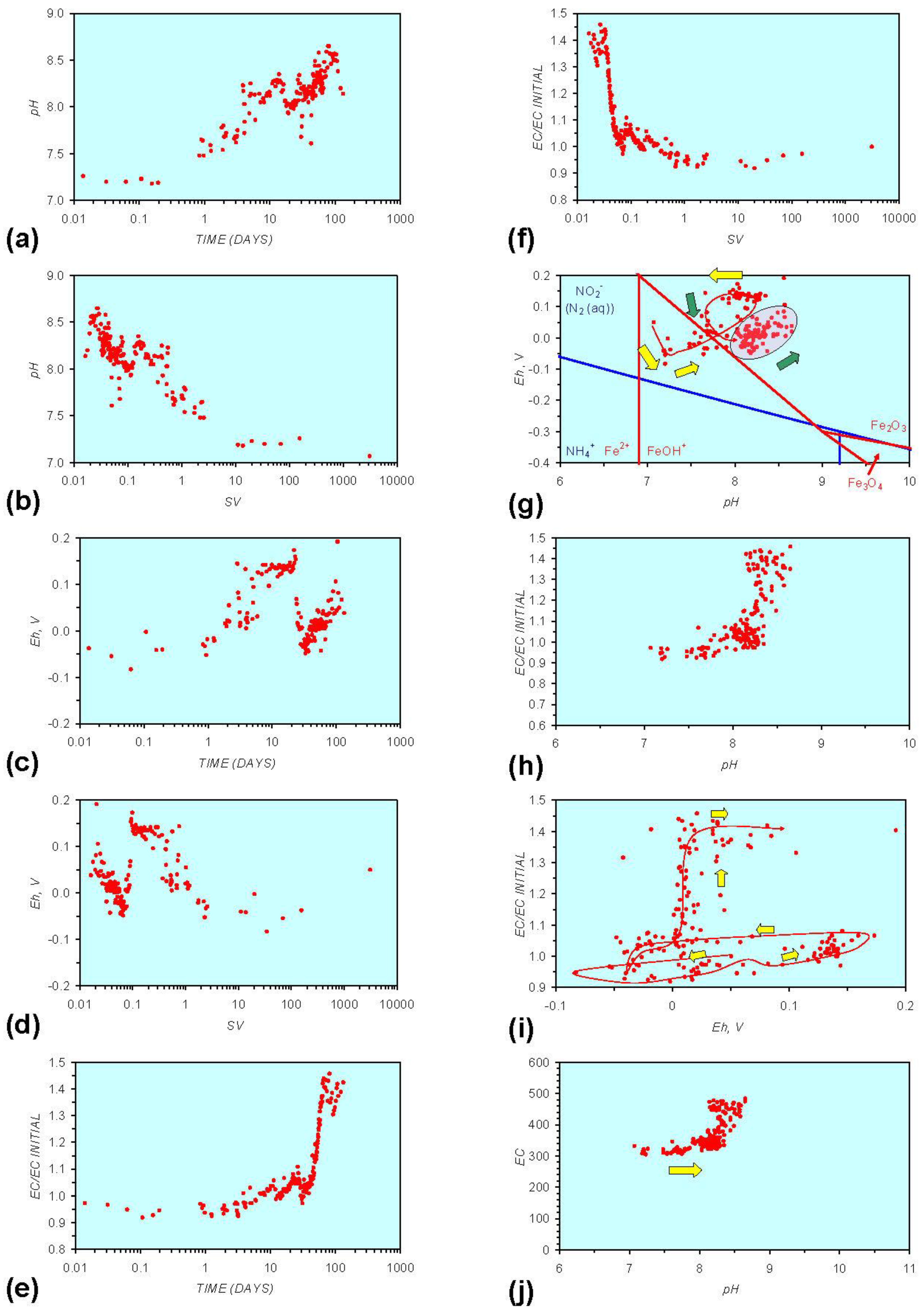
Figure A6.
MR6: n-Fe0, fresh water containing dissolved organic matter. (a) pH vs. Time; (b) pH vs. SV; (c) Eh vs. time; (d) Eh vs. SV; (e) EC/EC Initial vs. time; (f) EC/EC Initial vs. SV; (g) Eh vs. pH (SRE ringed); (h) pH vs. EC/EC Initial; (i) Eh vs. EC/EC Initial; (j) pH vs. E(C) Arrows indicate decreasing SV and increasing tim(e).

Figure A7.
MR7: n-Fe0, saline water. (a) pH vs. Time; (b) pH vs. SV; (c) Eh vs. time; (d) Eh vs. SV; (e) EC/EC Initial vs. time; (f) EC/EC Initial vs. SV; (g) Eh vs. pH (SRE ringed); (h) pH vs. EC/EC Initial; (i) Eh vs. EC/EC Initial; (j) pH vs. E(C) Arrows indicate decreasing SV and increasing tim(e).

Figure A8.
MR8: n-Fe0 + n-Cu0 + n-Al0, saline water. (a) pH vs. Time; (b) pH vs. SV; (c) Eh vs. time; (d) Eh vs. SV; (e) EC/EC Initial vs. time; (f) EC/EC Initial vs. SV; (g) Eh vs. pH (SRE ringed); (h) pH vs. EC/EC Initial; (i) Eh vs. EC/EC Initial; (j) pH vs. E(C) Arrows indicate decreasing SV and increasing tim(e).

Figure A9.
MR9: Ca-montmorillonite, fresh water. (a) pH vs. Time; (b) Eh vs. time; (c) EC/EC Initial vs. time; (d) Eh vs. pH (SRE ringed); (e) pH vs. EC/EC Initial; (f) Eh vs. EC/EC Initial; (g) pH vs. E(C) Arrows indicate decreasing SV and increasing tim(e).
Figure A9.
MR9: Ca-montmorillonite, fresh water. (a) pH vs. Time; (b) Eh vs. time; (c) EC/EC Initial vs. time; (d) Eh vs. pH (SRE ringed); (e) pH vs. EC/EC Initial; (f) Eh vs. EC/EC Initial; (g) pH vs. E(C) Arrows indicate decreasing SV and increasing tim(e).

Figure A10.
MR10: Ca-montmorillonite + n-Fe0, fresh water. (a) pH vs. Time; (b) pH vs. SV; (c) Eh vs. time; (d) Eh vs. SV; (e) EC/EC Initial vs. time; (f) EC/EC Initial vs. SV; (g) Eh vs. pH (SRE ringed); (h) pH vs. EC/EC Initial; (i) Eh vs. EC/EC Initial; (j) pH vs. E(C) Arrows indicate decreasing SV and increasing tim(e).

Figure A11.
MR11: Ca-montmorillonite + n-Fe0 + n-Cu0 + n-Al0, fresh water. (a) pH vs. Time; (b) pH vs. SV; (c) Eh vs. time; (d) Eh vs. SV; (e) EC/EC Initial vs. time; (f) EC/EC Initial vs. SV; (g) Eh vs. pH (SRE ringed); (h) pH vs. EC/EC Initial; (i) Eh vs. EC/EC Initial; (j) pH vs. E(C) Arrows indicate decreasing SV and increasing tim(e).

Figure A12.
MR12: Ca-montmorillonite, saline water. (a) pH vs. Time; (b) Eh vs. time; (c) EC/EC Initial vs. time; (d) Eh vs. pH (SRE ringed); (e) pH vs. EC/EC Initial; (f) Eh vs. EC/EC Initial; Arrows indicate decreasing SV and increasing tim(e).
Figure A12.
MR12: Ca-montmorillonite, saline water. (a) pH vs. Time; (b) Eh vs. time; (c) EC/EC Initial vs. time; (d) Eh vs. pH (SRE ringed); (e) pH vs. EC/EC Initial; (f) Eh vs. EC/EC Initial; Arrows indicate decreasing SV and increasing tim(e).

Figure A13.
MR13: Ca-montmorillonite + n-Fe0, saline water. (a) pH vs. Time; (b) pH vs. SV; (c) Eh vs. time; (d) Eh vs. SV; (e) EC/EC Initial vs. time; (f) EC/EC Initial vs. SV; (g) Eh vs. pH (SRE ringed); (h) pH vs. EC/EC Initial; (i) Eh vs. EC/EC Initial; (j) pH vs. E(C) Arrows indicate decreasing SV and increasing tim(e).

Figure A14.
MR14: Ca-montmorillonite + n-Fe0 + n-Cu0, saline water. (a) pH vs. Time; (b) pH vs. SV; (c) Eh vs. time; (d) Eh vs. SV; (e) EC/EC Initial vs. time; (f) EC/EC Initial vs. SV; (g) Eh vs. p(H) The redox trajectory ends in an SRE with a stable pH and decreasing Eh with time; (h) pH vs. EC/EC Initial; (i) Eh vs. EC/EC Initial; (j) pH vs. E(C) Arrows indicate decreasing SV and increasing tim(e).

Figure A15.
MR15: Ca-montmorillonite + n-Fe0 + n-Al0, saline water. (a) pH vs. Time; (b) pH vs. SV; (c) Eh vs. time; (d) Eh vs. SV; (e) EC/EC Initial vs. time; (f) EC/EC Initial vs. SV; (g) Eh vs. pH (SRE ringed); (h) pH vs. EC/EC Initial; (i) Eh vs. EC/EC Initial; (j) pH vs. E(C) Arrows indicate decreasing SV and increasing tim(e).

Figure A16.
MR11: Ca-montmorillonite + n-Fe0 + n-Cu0 + n-Al0, saline water. (a) pH vs. Time; (b) pH vs. SV; (c) Eh vs. time; (d) Eh vs. SV; (e) EC/EC Initial vs. time; (f) EC/EC Initial vs. SV; (g) Eh vs. pH (SRE ringed); (h) pH vs. EC/EC Initial; (i) Eh vs. EC/EC Initial; (j) pH vs. E(C) Arrows indicate decreasing SV and increasing tim(e).

© 2011 by the authors; licensee MDPI, Basel, Switzerland. This article is an open access article distributed under the terms and conditions of the Creative Commons Attribution license (http://creativecommons.org/licenses/by/3.0/).
Share and Cite
MDPI and ACS Style
Antia, D.D.J. Modification of Aquifer Pore-Water by Static Diffusion Using Nano-Zero-Valent Metals. Water 2011, 3, 79-112. https://doi.org/10.3390/w3010079
AMA Style
Antia DDJ. Modification of Aquifer Pore-Water by Static Diffusion Using Nano-Zero-Valent Metals. Water. 2011; 3(1):79-112. https://doi.org/10.3390/w3010079
Chicago/Turabian StyleAntia, David D. J. 2011. "Modification of Aquifer Pore-Water by Static Diffusion Using Nano-Zero-Valent Metals" Water 3, no. 1: 79-112. https://doi.org/10.3390/w3010079