Evaluating Hydrologic Response of an Agricultural Watershed for Watershed Analysis

Abstract

This paper describes the hydrological assessment of an agricultural watershed in the Midwestern United States through the use of a watershed scale hydrologic model. The Soil and Water Assessment Tool (SWAT) model was applied to the Maquoketa River watershed, located in northeast Iowa, draining an agriculture intensive area of about 5,000 km². The inputs to the model were obtained from the Environmental Protection Agency’s geographic information/database system called Better Assessment Science Integrating Point and Nonpoint Sources (BASINS). Meteorological input, including precipitation and temperature from six weather stations located in and around the watershed, and measured streamflow data at the watershed outlet, were used in the simulation. A sensitivity analysis was performed using an influence coefficient method to evaluate surface runoff and baseflow variations in response to changes in model input hydrologic parameters. The curve number, evaporation compensation factor, and soil available water capacity were found to be the most sensitive parameters among eight selected parameters. Model calibration, facilitated by the sensitivity analysis, was performed for the period 1988 through 1993, and validation was performed for 1982 through 1987. The model was found to explain at least 86% and 69% of the variability in the measured streamflow data for calibration and validation periods, respectively. This initial hydrologic assessment will facilitate future modeling applications using SWAT to the Maquoketa River watershed for various watershed analyses, including watershed assessment for water quality management, such as total maximum daily loads, impacts of land use and climate change, and impacts of alternate management practices.

1. Introduction

Hydrology is the main governing backbone of all kinds of water movement and hence of water-related pollutants. Understanding the hydrology of a watershed and modeling different hydrological processes within a watershed are therefore very important for assessing the environmental and economical well-being of the watershed. Simulation models of watershed hydrology and water quality are extensively used for water resources planning and management. These models can offer a sound scientific framework for watershed analyses of water movement and provide reliable information on the behavior of the system. New developments in modeling systems have increasingly relied on geographic information systems (GIS) that have made large area simulations feasible, and on database management systems such as Microsoft Access to support modeling and analysis. Furthermore, models can save time and money because of their ability to perform long-term simulations of the effects of watershed processes and management activities on water quantity, quality, and on soil quality [1].

Several watershed-scale hydrologic and water quality models such as HSPF (Hydrological Simulation Program—FORTRAN) [2], HEC-HMS (Hydrologic Modeling System) [3], CREAMS (Chemical, Runoff, and Erosion from Agricultural Management Systems) [4], EPIC (Erosion-Productivity Impact Calculator) [5], and AGNPS (Agricultural Non-Point Source) [6] have been developed for watershed analyses. While these models are very useful, they are generally limited in several aspects of watershed modeling, such as inappropriate scale, inability to perform continuous-time simulations, inadequate maximum number of subwatersheds, and the inability to characterize the watershed in enough spatial detail [7]. A relatively recent model developed by the U.S. Department of Agriculture (USDA) called SWAT (Soil and Water Assessment Tool) [8] has proven very successful in the watershed assessment of hydrology and water quality. According to [9], the wide range of SWAT applications underscores that usefulness of model as a robust tool to deal with variety of watershed problems. SWAT is a physically based model and offers continuous-time simulation, a high level of spatial detail, unlimited number of watershed subdivisions, efficient computation, and the capability of simulating changes in land management. An early application of the model by [10] compared the results of SWAT to historical streamflow and groundwater flow in three Illinois watersheds. The model was validated against measured streamflow and sediment loads across the entire U.S. [11]. The effect of spatial aggregation on SWAT was examined by [12,13]. The SWAT model was successfully applied to assess the impact of climate change in hydrology of the Upper Mississippi River Basin [14] and the Missouri River Basin [15]. SWAT has been chosen by the Environmental Protection Agency to be one of the models of their Better Assessment Science Integrating Point and Nonpoint Sources (BASINS) modeling package [16]. Gassman et al. [9] has provided a comprehensive list of SWAT model application and categorized them under major study areas. A search tool is placed at the Iowa State University’s website [17] where all up-to-date SWAT articles could be searched and retrieved.

Besides successful application of physically based models, there are several issues that question the model output such as uncertainty in input parameters, nonlinear relationships between hydrologic input features and hydrologic response, and the required calibration of numerous model parameters. These issues can be examined with sensitivity analyses of the model parameters to identify sensitive parameters with respect to their impact on model outputs. Proper attention to the sensitive parameters may lead to a better understanding and to better estimated values and thus to reduced uncertainty [18]. Knowledge of sensitive input parameters is beneficial for model development and leads to a model’s successful application. Arnold et al. [19] performed a sensitivity analysis of three hydrologic input parameters of the SWAT model against surface runoff, baseflow, recharge, and soil evapotranspiration on three different basins within the Upper Mississippi River Basin. Spruill et al. [20] selected fifteen hydrologic input variables of the SWAT model and varied them individually within acceptable ranges to determine model sensitivity in daily streamflow simulation. They found that the determination of accurate parameter values is vital for producing simulated streamflow data in close agreement with measured streamflow data. Two simple approaches of sensitivity analysis were compared using the SWAT model on an artificial catchment [18]. In both approaches, one parameter was varied at a time while holding the others fixed except that the way of defining the range of variation was different: the first approach varied the parameters by a fixed percentage of the initial value and the second approach varied the parameters by a fixed percentage of the valid parameter range. They found similar results for both approaches and suggested that the parameter sensitivity may be determined without the results being influenced by the chosen method. The paper identified several most sensitive hydrologic and plant-specific parameters but emphasized that sensitivities can be different for a natural catchment because of oversimplification of the processes in the chosen artificial catchment. Sexton et al. [21] used the mean value first-order reliability method to determine the contribution of parameter uncertainty to total model uncertainty in streamflow, sediment and nutrients outputs in a small Maryland watershed. Shen et al. [22] used the First-Order Error Analysis method to analyze the effect of parameter uncertainty on model outputs. Zhang et al. [23] used genetic algorithms and Bayesian Model Averaging to simultaneously conduct calibration and uncertainty analysis. Tolson and Shoemaker [24] compared two approaches of uncertainty analysis and fond dynamically dimensional search (DDS) more efficient than traditional generalized likelihood uncertainty estimation (GLUE) technique. Similarly, various tools and techniques have been used to assess model parameter sensitivity and for uncertainty analysis.

In this study, SWAT was applied to the Maquoketa River watershed, located in northeast Iowa (Figure 1). The goal of this study is to understand the complex interrelationships between topography, land use, soil characteristics and climate with respect to the hydrological response of the watershed. The specific objectives were to identify the SWAT’s hydrologic sensitive parameters relative to the estimation of surface runoff and baseflow, and to calibrate and validate the model for streamflow. The influence coefficient method was used to examine surface runoff and baseflow responses to changes in model input parameters. The parameters were ranked according to the magnitudes of response variable sensitivity to each of the model parameters, which divide high and low sensitivities. The SWAT model was calibrated by varying the values of sensitive parameters (as identified in the sensitivity analysis) within their permissible values and then compared simulated streamflow with the measured streamflow at the watershed outlet. This modeling application study facilitates future applications of the SWAT model for watershed-based hydrological assessment and solving agricultural water quality problems in the agricultural region.

Figure 1. Location of the Maquoketa River watershed (Northeast Iowa), and weather stations.

Figure 1. Location of the Maquoketa River watershed (Northeast Iowa), and weather stations.

2. Materials and Methods

2.1. SWAT Model Description

The SWAT model is a long-term, continuous simulation watershed model. It operates on a daily time step and is designed to predict the impact of management on water, sediment, and agricultural chemical yields. The model is physically based, computationally efficient, and capable of simulating a high level of spatial detail by allowing the division of watersheds into smaller subwatersheds. SWAT models water flow, sediment transport, crop/vegetation growth, and nutrient cycling. The model allows users to model watersheds with less monitoring data and to assess predictive scenarios using alternative input data such as climate, land-use practices, and land cover on water movement, nutrient cycling, water quality, and other outputs. Major model components include weather, hydrology, soil temperature, plant growth, nutrients, pesticides, and land management. Several model components have been previously validated for a variety of watersheds.

In SWAT, a watershed is divided into multiple subwatersheds, which are then further subdivided into Hydrologic Response Units (HRUs) that consist of homogeneous land use, management, and soil characteristics. The HRUs represent percentages of the subwatershed area and are not identified spatially within a SWAT simulation. The water balance of each HRU in the watershed is represented by four storage volumes: snow, soil profile (0–2 meters), shallow aquifer (typically 2–20 meters), and deep aquifer (more than 20 meters). The soil profile can be subdivided into multiple layers. Soil water processes include infiltration, evaporation, plant uptake, lateral flow, and percolation to lower layers. Flow, sediment, nutrient, and pesticide loadings from each HRU in a subwatershed are summed, and the resulting loads are routed through channels, ponds, and/or reservoirs to the watershed outlet. Detailed descriptions of the model and model components can be found in [8,25].

2.2. Maquoketa River Watershed and SWAT Input Data

The Maquoketa River watershed (MRW) covers 4,867 km² of predominantly agricultural land in northeast Iowa (Figure 1). The MRW is one of 13 tributaries of the Mississippi River that have been identified as contributing some of the highest levels of suspended sediments, nitrogen, and phosphorus to the Mississippi stream system [26]. These pollution loads are attributed mainly to agricultural nonpoint sources and result in degraded water quality within each watershed, in the Mississippi River, and ultimately in the Gulf of Mexico.

Land use, soil, and topography data required for simulating the watershed were obtained from the BASINS package [27]. Topographic information is provided in BASINS in the form of Digital Elevation Model (DEM) data. The DEM data were used to generate variations in subwatershed configurations such as subwatershed delineation, stream network delineation, and slope and slope lengths using the ArcView interface for the SWAT model (AVSWAT) [28]. Land-use categories provided in BASINS are relatively simplistic, including only one category for agricultural land (defined as “Agricultural Land-Generic” or AGRL). Agricultural lands cover almost 90% of the MRW; the remaining area is mostly forest. The soil data available in BASINS comes from the State Soil Geographic (STATSGO) database [29], which contains soil maps at a 1:250,000 scale. Each STATSGO map unit is linked to the Soil Interpretations Record attribute database that provides the proportionate extent of the component soils and soil layer properties. The STATSGO soil map units and associated layer data were used to characterize the simulated soils for the SWAT analyses.

The daily climate inputs consist of precipitation, maximum and minimum temperatures, solar radiation, wind speed, and relative humidity. In case of missing observed data or the absence of complete data, the weather generator within SWAT uses its statistical database to generate representative daily values for the missing variables for each subwatershed. Historical daily precipitation and daily maximum and minimum temperatures were obtained from the Iowa weather database [30] for the six climate stations located in or near the watershed (see Figure 1). The management operations required for the HRUs were defaulted by AVSWAT and consisted simply of planting, harvesting, and automatic fertilizer applications for the agricultural HRUs.

2.3. Influence Coefficient Method

The influence coefficient method is one of the most common methods for computing sensitivity coefficients in surface and ground water problems [31]. The method evaluates the sensitivity by changing each of the independent variables, one at a time. A sensitivity coefficient represents the change of a response variable that is caused by a unit change of an explanatory variable, while holding the rest of the parameters constant:

$$\frac{\Delta F}{\Delta P}=\frac{F\left(P_1,P_2,\mathrm{...},P_i+\Delta P_i,\mathrm{....}PN\right)-F\left(P_1,P_2,\mathrm{...},P_i,\mathrm{....}PN\right)}{\Delta P_i}$$

(1)

where F is the response variable, P is the independent parameter, and N is the number of parameters considered. The sensitivity coefficients can be positive or negative. A negative coefficient indicates an inversely proportional relation between a response variable and an explanatory parameter.

To meaningfully compare different sensitivities, the sensitivity coefficient was normalized by reference values, which represent the ranges of each pair of dependent variable and independent parameter. The normalized sensitivity coefficient is called the sensitivity index and is given as [32]:

$$s_i=\frac{P_m}{F_m}\frac{\Delta F}{\Delta P}$$

(2)

where s_i is the sensitivity index, and F_m and P_m are the mean of lowest and highest values of the selected range for the explanatory parameter and the response variable, respectively. A higher absolute value of sensitivity index indicates higher sensitivity and a negative sign shows inverse proportionality.

2.4. Simulation Approach

The AVSWAT model (ArcView interface of the SWAT model) was used in the watershed delineation process, which includes processing of DEM data for stream network delineation followed by subwatershed delineation. A total of 25 subwatersheds were delineated for the entire MRW (see Figure 1). The subwatersheds were then further subdivided into HRUs that were created for each unique combination of land use and soil. Recommended thresholds of 10% for land cover and 5% for the soil area were applied to limit the number of HRUs in each subwatershed.

After the model setup, SWAT was executed with the following simulations options: (1) the Runoff Curve Number method for estimating surface runoff from precipitation, (2) the Hargreaves method for estimating potential evapotranspiration generation, and (3) the variable-storage method to simulate channel water routing. A simulation period of 1988 through 1993 was selected for the sensitivity analysis. Several model runs were executed for each input parameter with a range of values, keeping simulation options and other parameters’ values constant. The sensitivity index was calculated for each parameter from the average annual values for surface runoff and baseflow separately. The analysis provided information on the most to least sensitive parameters for flow response of the watershed.

Facilitated by the sensitivity analysis, the model was calibrated for the same period against the measured streamflow data at the U.S. Geological Survey (USGS) stream gage (Station # 05418500). The model was then validated for the period 1982 through 1987. Two statistical approaches were used to evaluate the model performance: coefficient of determination (R²) and Nash-Sutcliffe simulation efficiency (E). The R² value is an indicator of the strength of relationship between the observed and simulated values; and, E indicates how well the plot of observed versus simulated value fits the 1:1 line. If the R² value is close to zero and the E value is less than or close to zero, the model prediction is considered unacceptable. If the values approach one, the model predictions become perfect.

3. Results and Discussion

3.1. Sensitivity Analysis

A total of eight model input parameters were selected for sensitivity analysis based on extensive literature review on potential sensitive parameters of the SWAT model. These were curve number (CN), soil evaporation compensation factor (ESCO), plant uptake compensation factor (EPCO), soil available water capacity (SOL_AWC), baseflow alpha factor (ALPHA_BF), groundwater revap coefficient (GW_RAVAP), and deep aquifer percolation coefficient (RECHRG_DP). Table 1 lists the model parameters along with their initial estimates and acceptable ranges. Details on the model parameters and their functions can be found in [20]. The initial estimate value of a model parameter is the average and most applicable value for that particular parameter and is defaulted by the model interface. Most of the model inputs in the SWAT model are process-based except for a few important variables such as runoff curve number, evaporation coefficients, and others that are not well defined physically. These parameters, therefore, must be constrained by their applicability limits.

In the sensitivity analysis, surface runoff and baseflow were treated as the response or dependent variables, while model parameters were the explanatory or independent variables. The sensitivity coefficients and indices were examined to characterize surface runoff and baseflow under different parameter ranges. Table 2 summarizes the sensitivity coefficients and sensitivity indices of all parameters corresponding to the changes in surface runoff and baseflow volumes in response to changes in the model parameter. In general, the higher the absolute values of the sensitivity index, the higher the sensitivity of the corresponding parameter. A negative sign indicates an inverse relationship between the parameter and response variable. Results in Table 2 indicate that the surface runoff was sensitive, from most to least, to CN, ESCO, SOL_AWC, and EPCO for the selected variation range, while baseflow was sensitive, from most to least, to CN, ESCO, SOL_AWC, RECHRG_DP, GW_REVAP, ALPHA_BF, and GW_DELAY. Surface runoff was not found directly sensitive to ALPHA_BF, GW_REVAP, GW_DELAY, and RECHARG_DP, while baseflow was sensitive to all parameters considered in this study.

Table 1. Parameter ranges and initial values used in the sensitivity analysis.

Model parameter	Variable name	Range	Model initial estimates
Curve Number (for AGRL)	CN	69–85	77
Soil evaporation compensation factor	ESCO	0.75–0.95	0.95
Plant uptake compensation factor	EPCO	0.01–1	1.0
Soil available water capacity (mm)	SOL_AWC	±0.04	-
Baseflow alpha factor	ALPHA_BF	0.05–0.8	0.048
Groundwater revap coefficient	GW_REVAP	0.02–0.2	0.02
Groundwater delay time (day)	GW_DELAY	0–100	31
Deep aquifer percolation fraction	RECHRG_DP	0–1	0.05

Table 1. Parameter ranges and initial values used in the sensitivity analysis.

Model parameter	Variable name	Range	Model initial estimates
Curve Number (for AGRL)	CN	69–85	77
Soil evaporation compensation factor	ESCO	0.75–0.95	0.95
Plant uptake compensation factor	EPCO	0.01–1	1.0
Soil available water capacity (mm)	SOL_AWC	±0.04	-
Baseflow alpha factor	ALPHA_BF	0.05–0.8	0.048
Groundwater revap coefficient	GW_REVAP	0.02–0.2	0.02
Groundwater delay time (day)	GW_DELAY	0–100	31
Deep aquifer percolation fraction	RECHRG_DP	0–1	0.05

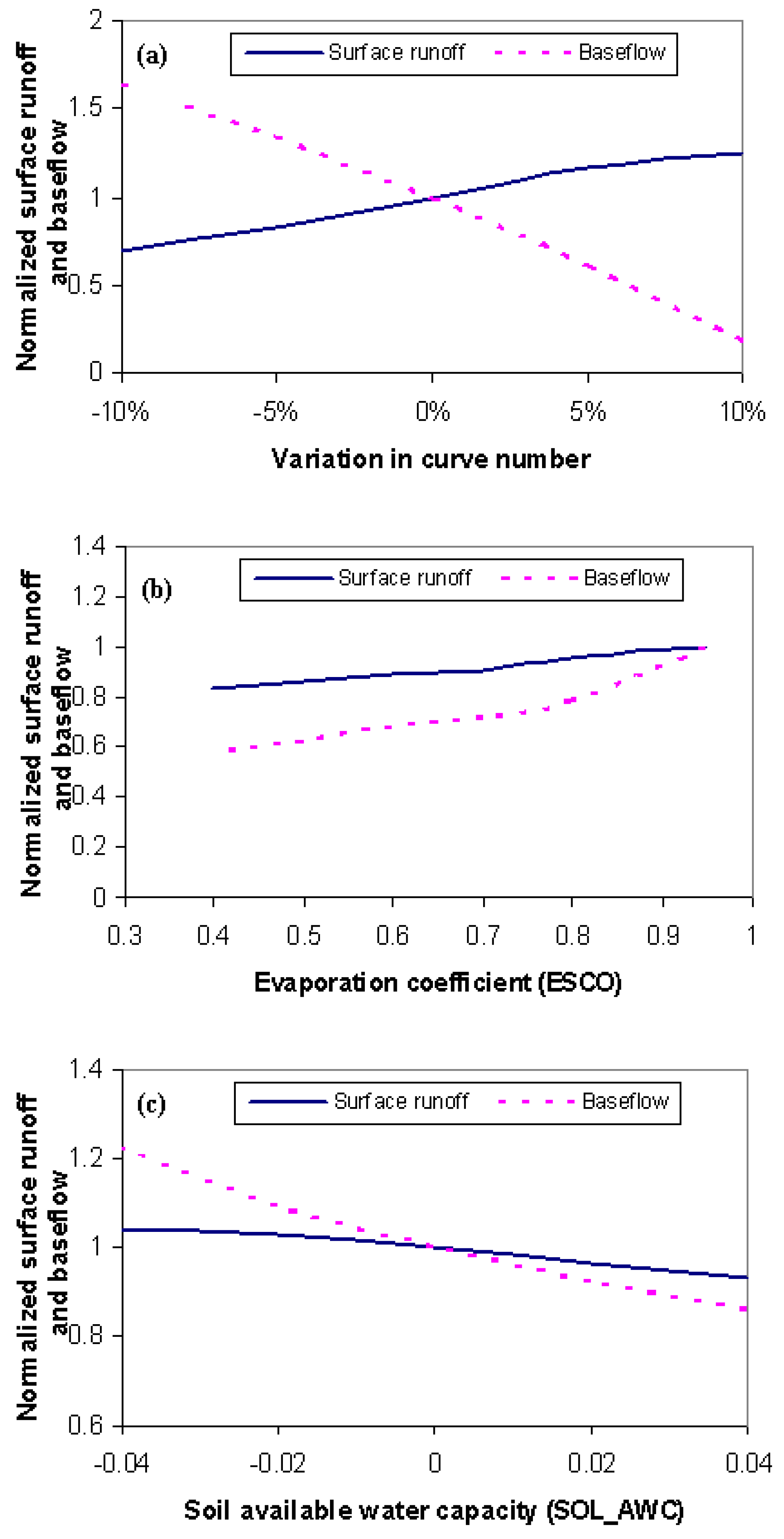
Further analysis was conducted for the top three most influencing parameters: CN, ESCO, and SOL_AWC. CN, an empirically established dimensionless number, is related to land use, soil type, and antecedent moisture condition, and is well-accepted for rainfall-runoff modeling. Figure 2(a) shows the response of surface runoff and baseflow when CN was changed from −10% to +10% with an increment of 5%. As expected, higher CN values resulted in increased surface runoff and decreased baseflow, and vice versa; but the rate of change of surface runoff was not consistent with that of baseflow. Baseflow was found to be affected more than surface runoff for different CN values.

Figure 2(b) shows the impact of ESCO on surface runoff and baseflow as its value decreased from defaulted 0.95 to lower values. ESCO adjusts the depth distribution for evaporation from the soil to account for the effect of capillary action, crusting, and cracking. Decreasing ESCO allows lower soil layers to compensate for a water deficit in upper layers and causes higher soil evapotranspiration, which in turn reduces both surface runoff and baseflow. ESCO was found to have a higher impact on baseflow than surface runoff as evident by the rate of decrease in flow values (Figure 2(b)).

Figure 2. Sensitivity of surface runoff and baseflow to (a) CN, (b) ESCO, and (c) SOL_AWC.

Figure 2. Sensitivity of surface runoff and baseflow to (a) CN, (b) ESCO, and (c) SOL_AWC.

Table 2. Sensitivity indices of model parameters.

Parameter	Initial value	Parameter				Response variable (Surface Runoff)						Response variable (Baseflow)
		P1	P2	ΔP	MeanPm	F1	F2	ΔF	MeanFm	$\frac{\Delta F}{\Delta P}$	$\frac{P_m}{F_m}\frac{\Delta F}{\Delta P}$	F1	F2	ΔF	MeanFm	$\frac{\Delta F}{\Delta P}$	$\frac{P_m}{F_m}\frac{\Delta F}{\Delta P}$
CN	77	85	69	16	77	310	173	137	241	8.57	2.73	21	181	−160	101	−10.0	−7.63
ESCO	0.95	0.5	1	0.5	0.75	214	249	−34	231	−68.9	−0.22	69	110	−41	90	−82.2	−0.69
EPCO	1	0.01	1	0.99	0.505	264	249	15	256	15.09	0.03	124	110	14	117	14.1	0.06
SOL_AWC		0.04	−0.04	0.08	0.04	232	259	−27	246	−336	−0.05	95	135	−40	115	−503	−0.17
ALPHA_BF	0.048	0.048	0.8	0.75	0.424	249	249	0	249	0	0	110	114	−4	112	−4.7	−0.02
GW_REVAP	0.02	0.02	0.2	0.18	0.11	249	249	0	249	0	0	110	95	15	102	85.6	0.09
GW_DELAY	31	0	100	100	50	249	249	0	249	0	0	108	106	1	108	0.0	0.01
RECHARG_DP	0.05	0	1	1	0.5	249	249	0	249	0	0	113	91	22	102	22.3	0.11

Table 2. Sensitivity indices of model parameters.

Parameter	Initial value	Parameter				Response variable (Surface Runoff)						Response variable (Baseflow)
		P1	P2	ΔP	MeanPm	F1	F2	ΔF	MeanFm	$\frac{\Delta F}{\Delta P}$	$\frac{P_m}{F_m}\frac{\Delta F}{\Delta P}$	F1	F2	ΔF	MeanFm	$\frac{\Delta F}{\Delta P}$	$\frac{P_m}{F_m}\frac{\Delta F}{\Delta P}$
CN	77	85	69	16	77	310	173	137	241	8.57	2.73	21	181	−160	101	−10.0	−7.63
ESCO	0.95	0.5	1	0.5	0.75	214	249	−34	231	−68.9	−0.22	69	110	−41	90	−82.2	−0.69
EPCO	1	0.01	1	0.99	0.505	264	249	15	256	15.09	0.03	124	110	14	117	14.1	0.06
SOL_AWC		0.04	−0.04	0.08	0.04	232	259	−27	246	−336	−0.05	95	135	−40	115	−503	−0.17
ALPHA_BF	0.048	0.048	0.8	0.75	0.424	249	249	0	249	0	0	110	114	−4	112	−4.7	−0.02
GW_REVAP	0.02	0.02	0.2	0.18	0.11	249	249	0	249	0	0	110	95	15	102	85.6	0.09
GW_DELAY	31	0	100	100	50	249	249	0	249	0	0	108	106	1	108	0.0	0.01
RECHARG_DP	0.05	0	1	1	0.5	249	249	0	249	0	0	113	91	22	102	22.3	0.11

Similarly, sensitivity of the model to SOL_AWC values from the default is shown in Figure 2(c). Higher values of SOL_AWC means higher capacity of soil to hold water and thereby causing less water available for surface runoff and percolation, and vice versa. As can be seen in Figure 2(c), increase in values of SOL_AWC leads to decrease in both surface runoff and baseflow. Opposite trend can be seen for decrease in SOL_AWC values, but the rate of change was found to be different. While surface runoff was found to be affected same way for both increase and decrease of SOL_AWC, baseflow was found to be affected more for decreasing SOL_AWC. In any case, baseflow was again found to be affected more than surface runoff.

While sensitivity analysis is a routine process, it is imperative for successful calibration and application of the model. Sensitivity of a parameter in one watershed may not reflect the same level of sensitivity on another watershed. It can vary from watershed to watersheds and therefore needs to be examined thoroughly before the calibration starts.

3.2. Calibration and Validation

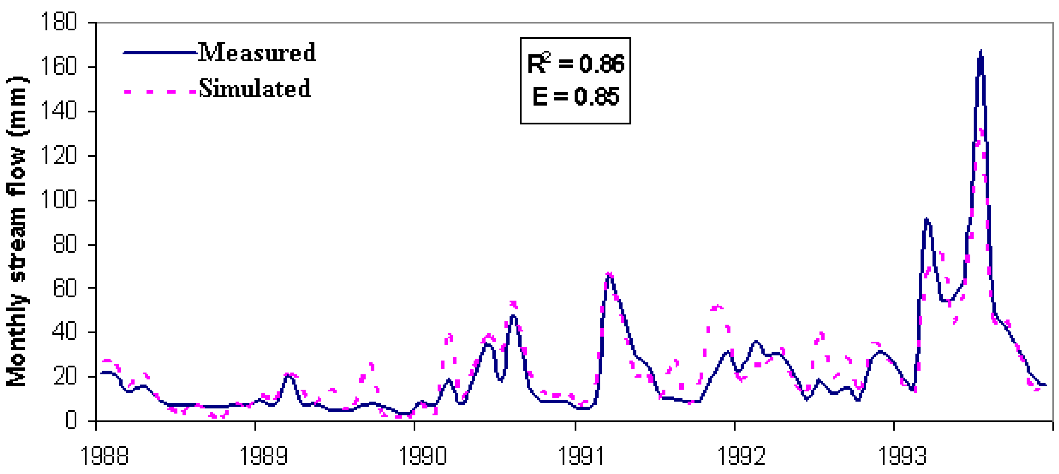
Calibration of the model was performed by comparing the simulated streamflow with the monitoring data from the field. Measured data at the watershed outlet (USGS gaging station # 05418500, Maquoketa River near Maquoketa, Iowa) was divided into two groups including variations of wet, dry and normal years. Years 1988 to 1993 were selected for calibration while years 1982 to 1987 for validation. During the calibration process, the model’s input parameters were adjusted, as guided by the sensitivity analysis, to match the observed and simulated streamflows. Table 3 lists the final calibrated values of the model variables. A time-series plot of the measured and simulated monthly streamflows (Figure 3) shows that the magnitude and trend in the simulated monthly flows closely followed the measured data most of the time. The measured and simulated average monthly flow volumes were 22.28 and 24.08 mm, respectively. The statistical evaluation yielded an R² value of 0.86 and an E value of 0.85, indicating a strong correlation between the measured and predicted flows.

Table 3. Final calibrated values of SWAT parameters for Maquoketa River watershed.

Parameter	Value
CN (for AGRL only)	72
ESCO	0.85
SOL_AWC	−0.04
GW_REVAP	0.15
GW_DELAY	50
RECHRG_DP	0.5

Table 3. Final calibrated values of SWAT parameters for Maquoketa River watershed.

Parameter	Value
CN (for AGRL only)	72
ESCO	0.85
SOL_AWC	−0.04
GW_REVAP	0.15
GW_DELAY	50
RECHRG_DP	0.5

Figure 3. Monthly time series of predicted and measured streamflow at USGS gauge 05418500 (watershed outlet) for the 1988-93 calibration period.

Figure 3. Monthly time series of predicted and measured streamflow at USGS gauge 05418500 (watershed outlet) for the 1988-93 calibration period.

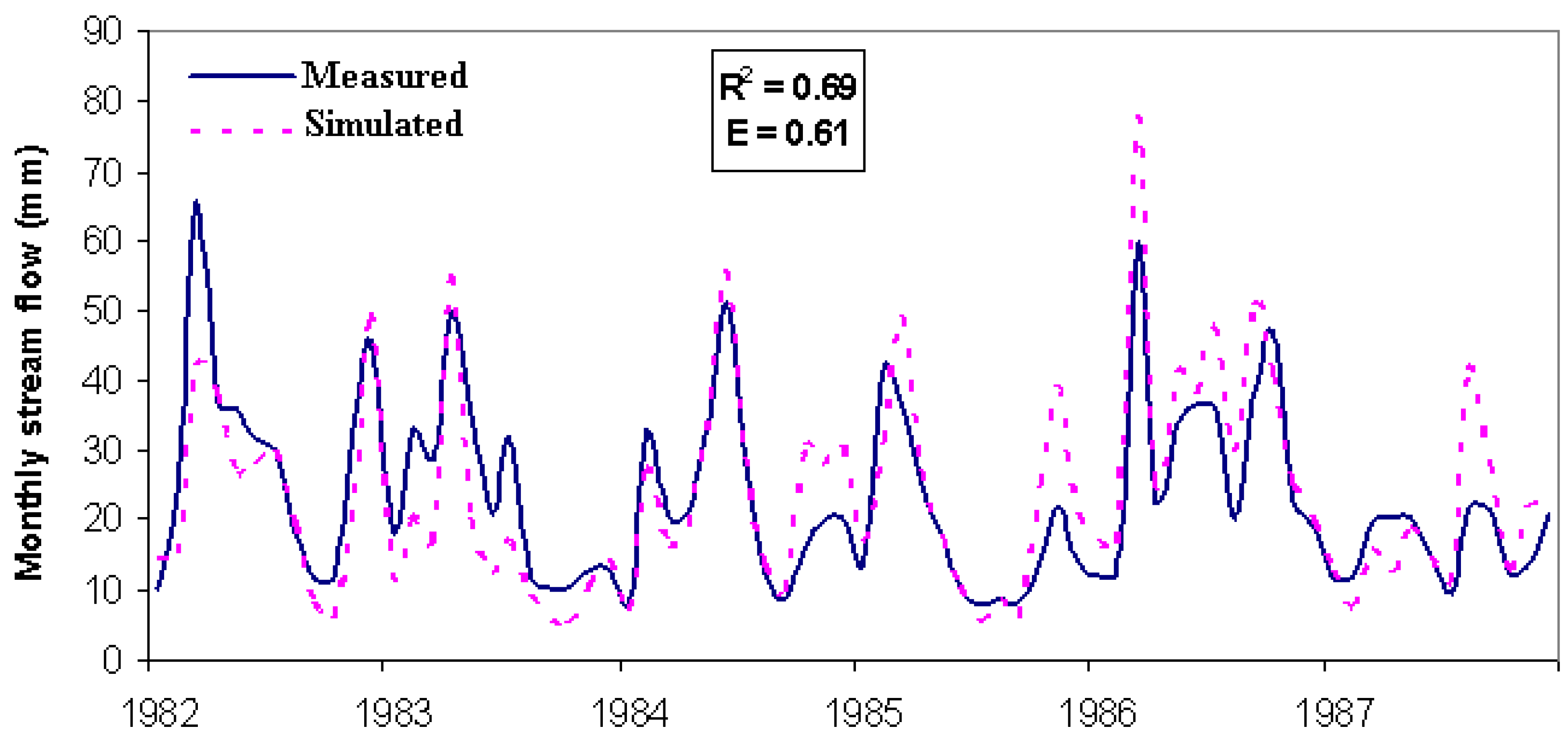
Figure 4. Monthly time series of predicted and measured streamflow at USGS gauge 05418500 (watershed outlet) for the 1982-87 validation period.

Figure 4. Monthly time series of predicted and measured streamflow at USGS gauge 05418500 (watershed outlet) for the 1982-87 validation period.

During the validation process, the model was run with input parameters set during the calibration process without any change. All input data including land use and soil was considered stationary except the meteorological inputs. Figure 4 shows the time-series plot of simulated versus measured monthly streamflow. The measured and simulated average monthly flow volumes for the validation period were 23.40 and 23.44 mm, respectively. The R² and E values between the measured and simulated streamflows were 0.69 and 0.61, respectively. Statistical evaluation of the model output for both calibration and validation was found to satisfy the criteria suggested by Moriasi et al. [1].

It is emphasized that the hydrological calibration is the first step in understanding the complex hydro-geological process of the watershed. Sensitivity analysis of model parameters helps understand response behavior of the watershed due to complex hydro-geologic interactions. Once the hydrologic condition represented by the model is satisfied, the model can be taken to a next level for water quality analyses.

4. Conclusions

Information about a model’s sensitivity to input parameters benefits model development and leads to its successful application to solve water resources problems. This study assessed and identified sensitive hydrologic parameters of the SWAT model to using the influence coefficient method, as determined in an application to the agriculture dominated watershed (Maquoketa River watershed) in the Midwest United States. Surface runoff was found to be sensitive, from most to least, to CN, ESCO, SOL_AWC, and EPCO for the selected variation range, while baseflow was found to be sensitive, from most to least, to CN, ESCO, SOL_AWC, RECHRG_DP, GW_REVAP, ALPHA_BF, and GW_DELAY. Model sensitivities to the three most influencing parameters for both surface runoff and baseflow—CN, ESCO, and SOL_AWC—were further evaluated. Sensitivity analysis provides good insight into the model input parameters and demonstrates that the model is able to simulate hydrological processes very well. The output of this study is consistent with other studies which tested sensitivity of SWAT parameters. Among several studies, Arnold et al. [18] and Spruill et al. [19] also found the same top three parameters, CN, ESCO and SOL_AWC, to be the most sensitive parameters to consider for hydrological response of the watershed.

Based on the assessment of model parameters to which the model is most to least sensitive, SWAT was calibrated and validated for streamflow at the watershed outlet. The calibration process used measured data for the period 1988–1993 and yielded a strong correlation (R² = 0.86 and E = 0.85) between measured and simulated flow volumes. Model validation was performed for the period 1982–1987 and generated an R² value of 0.69 and E value of 0.61. This study indicates that the SWAT model can be an effective tool for accurately simulating the hydrology of the Maquoketa River watershed. Accurate flow simulations are required to accurately predict sediment loads and chemical concentrations, and to simulate various scenarios related to cropping and alternative management to mitigate water quality problems in the region.

References

- Moriasi, D.N.; Arnold, J.G.; Van Liew, M.W.; Bingner, R.L.; Harmel, R.D.; Veith, T.L. Model evaluation guidelines for systematic quantification of accuracy in watershed simulations. Trans. ASABE 2007, 50, 885–900. [Google Scholar] [CrossRef]
- Johansen, N.B.; Imhoff, J.C.; Kittle, J.L.; Donigian, A.S. Hydrologic Simulation Program—FORTRAN (HSPF): User’s Manual for Release 8; EPA-600/3-84-066; U.S.; Environmental Protection Agency: Athens, GA, USA, 1984. [Google Scholar]
- U.S. Army Corps of Engineers Hydrologic Engineering Center (USACE-HEC). In HEC-HMS Hydrologic Modeling System User’S Manual; USACE-HEC: Davis, CA, USA, 2000.
- CREAMS: A Field-Scale Model for Chemicals, Runoff, and Erosion from Agricultural Management Systems; Conservation Research Report No. 26; Knisel, W.G. (Ed.) USA-SEA: Washington, DC, USA, 1980.
- Williams, J.R.; Jones, C.A.; Dyke, P.T. A modeling approach to determining the relationship between erosion and soil productivity. Trans. ASAE 1984, 27, 129–144. [Google Scholar] [CrossRef]
- Young, R.A.; Onstad, C.A.; Bosch, D.D.; Anderson, W.P. AGNPS: A non-point source pollution model for evaluating agricultural watersheds. J. Soil Water Conserv. 1989, 44, 168–173. [Google Scholar]
- Saleh, A.; Arnold, J.G.; Gassman, P.W.; Hauck, L.M.; Rosenthal, W.D.; Williams, J.R.; McFarland, A.M.S. Application of SWAT for the Upper North Bosque River watershed. Trans. ASAE 2000, 43, 1077–1087. [Google Scholar] [CrossRef]
- Arnold, J.G.; Srinivasan, R.; Muttiah, R.S.; Williams, J.R. Large area hydrologic modeling and assessment Part I: Model development. J. Am. Water Resour. Assoc. 1998, 34, 73–89. [Google Scholar] [CrossRef]
- Gassman, P.W.; Reyes, M.; Green, C.H.; Arnold, J.G. The Soil and Water Assessment Tool: Historical development, applications, and future directions. Trans. ASABE 2007, 50, 1211–1250. [Google Scholar] [CrossRef]
- Arnold, J.G.; Allen, P.M. Simulating hydrologic budgets for three Illinois watersheds. J. Hydrol. 1996, 176, 57–77. [Google Scholar] [CrossRef]
- Arnold, J.G.; Muttiah, R.S.; Srinivasan, R.; Allen, P.M. Regional estimation of base flow and groundwater recharge in the Upper Mississippi River Basin. J. Hydrol. 1999, 227, 21–40. [Google Scholar] [CrossRef]
- FitzHugh, T.W.; Mackay, D.S. Impacts of input parameter spatial aggregation on an agricultural nonpoint source pollution model. J. Hydrol. 2000, 236, 35–53. [Google Scholar] [CrossRef]
- Jha, M.K.; Gassman, P.W.; Secchi, S.; Gu, R.; Arnold, J.G. Effect of watershed subdivision on SWAT flow, sediment, and nutrient predictions. J. Am. Water Resour. Assoc. 2004, 40, 811–825. [Google Scholar] [CrossRef]
- Jha, M.K.; Pan, Z.; Takle, E.S.; Gu, R. Impacts of climate change on streamflow in the Upper Mississippi River Basin: A regional climate model perspective. J. Geophys. Res. 2004, 109, D09105. [Google Scholar]
- Stone, M.C.; Hotchkiss, R.H.; Hubbard, C.M.; Fontaine, T.A.; Mearns, L.O.; Arnold, J.G. Impacts of climate change on Missouri River basin water yield. J. Am. Water Resour. Assoc. 2001, 37, 1119–1130. [Google Scholar] [CrossRef]
- Whittemore, R.C. The BASINS Model. Water Environ. Technol. 1998, 10, 57–61. [Google Scholar]
- SWAT Literature Database for Peer-reviewed Articles. Available online: https://www.card.iastate.edu/swat_articles (accessed on 20 January 2011).
- Lenhart, T.; Eckhardt, K.; Fohrer, N.; Frede, H.-G. Comparison of two different approaches of sensitivity analysis. Phys. Chem. Earth 2002, 27, 645–654. [Google Scholar] [CrossRef]
- Arnold, J.G.; Srinivasan, R.; Muttiah, R.S.; Allen, P.M.; Walker, C. Continental scale simulation of the hydrologic balance. J. Am. Water Resour. Assoc. 1999, 35, 1037–1052. [Google Scholar] [CrossRef]
- Spruill, C.A.; Workman, S.R.; Taraba, J.L. Simulation of daily and monthly stream discharge from small watershed using the SWAT Model. Trans. ASAE 2000, 43, 1431–1439. [Google Scholar] [CrossRef]
- Sexton, A.M.; Shismohammadi, A.; Sedghi, A.M.; Montas, H.J. Impact of parameter uncertainty on critical SWAT output simulations. Trans. ASABE 2011, 54, 461–471. [Google Scholar] [CrossRef]
- Shen, Z.; Hong, Q.; Yu, H.; Niu, J. Parameter uncertainty analysis of non-point source pollution from different land use types. Sci. Total Environ. 2010, 408, 1971–1978. [Google Scholar] [CrossRef] [PubMed]
- Zhang, X.R.; Srinivasan, R.; Bosch, D. Calibration and uncertainty analysis of the SWAT model using Genetic Algorithms and Bayesian Model Averaging. J. Hydrol. 2009, 374, 307–317. [Google Scholar] [CrossRef]
- Tolson, B.A.; Shoemaker, C.A. Efficient prediction uncertainty approximation in the calibration of environmental simulation models. Water Resour. Res. 2008, 44, 1–19. [Google Scholar]
- Neitsch, S.L.; Arnold, J.G.; Kiniry, J.R.; Williams, J.R. Soil and Water Assessment Tool Theoretical Documentation, Version 2000; Blackland Research Center, Texas Agricultural Experiment Station: Temple, TX, USA, 2000. [Google Scholar]
- Upper Mississippi River Basin Loading Database (Nutrients and Sediments). Available online: http://www.umesc.usgs.gov/data_library/sediment_nutrients/sediment_nutrient_page.html (accessed on 20 January 2011).
- U.S. Environmental Protection Agency (USEPA). BASINS 3.0: Better Assessment Science Integrating Point and Nonpoint Sources; U.S. Environmental Protection Agency, Office of Water, Office of Science and Technology: Washington, DC, USA, 2001. [Google Scholar]
- Di Luzio, M.; Srinivasan, R.; Arnold, J.G.; Neitsch, S.L. Soil and Water Assessment Tool: ArcView GIS Interface Manual: Version 2000, GSWRL Report 02-03, BRC Report 02-07; Texas Water Resources Institute TR-193: College Station, TX, USA; 346.
- U.S. Department of Agriculture (USDA). State Soil Geographic (STATSGO) Data Base: Data Use Information; Miscellaneous Publication Number 1492; U.S. Department of Agriculture: Fort Worth, TX, USA, 1994. [Google Scholar]
- Iowa Environmental Mesonet—A weather database for the state of Iowa. Available online: http://www.mesonet.agron.iastate.edu (accessed on 20 January 2011).
- Helsel, D.R.; Hirsch, R.M. Statistical Methods in Water Resources; Elsevier: New York, NY, USA, 1992. [Google Scholar]
- Gu, R.; Li, Y. River temperature sensitivity to hydraulic and meteorological parameters. J. Environ. Manage. 2002, 66, 43–56. [Google Scholar] [CrossRef] [PubMed]
© 2011 by the authors; licensee MDPI, Basel, Switzerland. This article is an open access article distributed under the terms and conditions of the Creative Commons Attribution license (http://creativecommons.org/licenses/by/3.0/).
Share and Cite
MDPI and ACS Style
Jha, M.K. Evaluating Hydrologic Response of an Agricultural Watershed for Watershed Analysis. Water 2011, 3, 604-617. https://doi.org/10.3390/w3020604
AMA Style
Jha MK. Evaluating Hydrologic Response of an Agricultural Watershed for Watershed Analysis. Water. 2011; 3(2):604-617. https://doi.org/10.3390/w3020604
Chicago/Turabian StyleJha, Manoj Kumar. 2011. "Evaluating Hydrologic Response of an Agricultural Watershed for Watershed Analysis" Water 3, no. 2: 604-617. https://doi.org/10.3390/w3020604