Article

Mean Sea Level Variability and Influence of the North Atlantic Oscillation on Long-Term Trends in the German Bight

1
Research Institute for Water and Environment, University of Siegen, Paul-Bonatz-Str. 9-11, Siegen 57076, Germany
2
Federal Institute of Hydrology, Am Mainzer Tor 1, Koblenz 56068, Germany
*
Author to whom correspondence should be addressed.
Water 2012, 4(1), 170-195; https://doi.org/10.3390/w4010170
Submission received: 9 January 2012 / Revised: 30 January 2012 / Accepted: 13 February 2012 / Published: 24 February 2012
(This article belongs to the Special Issue Flood Risk Management)

Abstract

:
Changes in the seasonal cycle of mean sea level (MSL) may affect the heights of storm surges and thereby flood risk in coastal areas. This study investigates the intra- and inter-annual variability of monthly MSL and its link to the North Atlantic Oscillation using records from 13 tide gauges located in the German Bight. The amplitudes of the seasonal MSL cycle are not regionally uniform and vary between 20 and 29 cm. Generally, the amplitudes are smaller at the southwestern stations, increasing as one travels to the northeastern part. The amplitudes, as well as the phase of the seasonal cycle, are characterized by a large inter-annual and inter-decadal variability, but no long-term trend could be detected. Nevertheless, in the last two decades annual maximum peaks more frequently occurred in January and February, whereas beforehand an accumulation was detected for the November and December period. These changes in phase in the various sea level time series are consistent with a shift in the annual cycle, which is, however, not significant. The changes are associated with strongly increasing trends in monthly MSL of the winter season (J–M), which are considerably higher compared to the remaining seasons. For the same season, the MSL and North Atlantic Oscillation (NAO) indices show strong similarities, resulting in statistically significant correlations (r ~ 0.7). Hence, these changes are linked with changing pressure conditions over the North Atlantic, which lead to a strong phase of positive values in the NAO index between the 1960’s and 1990’s.

Graphical Abstract

1. Introduction

During the last century, coastal regions have been strongly governed by a rapid growth in populations and economic assets with increasing urbanization affecting the vulnerability. At the same time, global sea levels have risen as a result of a warming climate. Over the 20th century a significant rise in global mean sea level (MSL) has been detected by different authors using various techniques [1]. The results of these studies show a strong variability in the rates of rise that is far from linear with inter-annual fluctuations linked to regional climate patterns [2]. Furthermore, the rates of observed MSL vary across the globe with regions of increase and regions of decrease [3]. An extensive study addressing regional sea level development in the German Bight was conducted by Führböter and Jensen [4]. They analyzed mean tidal high water levels (MHW) and mean tidal low water levels (MLW) over a time span of about 140 years and found significant increasing trends for the MHW of about 2.5 mm/yr on average but no significant change in the MLW. Jensen and Mudersbach [5] updated and extended the study (in terms of the considered time period) and affirmed the key findings. They reported an increase in the mean tidal range (MTR) of about 10% since 1955 along the German North Sea coastline. Mean sea level changes in the German Bight have recently been investigated by Wahl et al. [6,7], based on MSL time series from 13 tide gauges covering the entire German Bight. The focus was on analyzing long-term changes, making use of different statistical techniques. They found two periods of accelerated sea level rise, one at the end of the 19th century and another covering recent decades with some differences along the coastline.
For coastal planning it is not only important to understand long-term changes in MSL but also short-term variability, e.g., on annual time scales. First studies on the intra-annual (seasonal) behavior of MLW and MHW in the German Bight were conducted by Jensen et al. [8]. The key findings can be summarized as follows: The minima for MHW usually occur between February and April, while the maxima occur between July and August. From the corresponding seasonal cycle for the MLW minima were detected in April or May and maxima in October or November. Anyway, until now no studies have been undertaken aimed at analyzing the seasonal cycle of the MSL in the German Bight in detail.
For a better understanding of sea level changes, high quality sea level observations are needed. Different external factors, such as atmospheric pressure variations or meteorological forces, may affect observed water levels. These factors have to be analyzed in detail to quantify their influence on different time scales. One common method of addressing external effects is the observation of major atmospheric modes of variability that can have significant effects on the variability of sea level on inter-annual and inter-decadal time scales [9]. The North Atlantic Oscillation (NAO), the El Nino-Southern Oscillation (ENSO) and the Northern Pacific Oscillation (NPO) are part of the global oscillation system. This global oscillation system has significant influences on weather and climate, including sea levels. For the investigation area considered for the present study (i.e., the German Bight), the NAO is the main oscillation of interest. Commonly, the different oscillations are addressed by a normalized index.
Many authors studied the influence of the NAO using different atmospheric factors, such as rainfall and temperature [10,11], wind and other meteorological parameters [12,13,14]. Further investigations on the link between NAO and Arctic ice export have been performed by Hilmer and Jung [15], while Petrow et al. [16] analyzed the relationship between changes in circulation patterns and flood hazard in Germany. Other publications indicate the influence of circulation patterns such as the NAO on sea level. Wakelin et al. [17] examined sea level dependence over the NW European Shelf and found varying correlations, which are positive in the northern region and strongly negative in the south. They measured sensitivity by looking at the seasonal (December to March) sea level changes (in mm) per unit NAO over the whole region by considering results from a tide and surge model. Highest sensitivities with values up to 96 mm per unit NAO have been detected for the German Bight. Woodworth et al. [18] investigated the dependence of sea level percentiles on the NAO in the North Sea and found a homogeneous distribution throughout the tidal range for the UK, but a larger dependence for extreme high waters compared to the median sea levels (MeSL) for the eastern parts of the North Sea (e.g., the German Bight). Yan et al. [19] and Jevrejeva et al. [20] noted that the relationship between NAO and sea level in the northern European parts is unsteady over time, with highest correlation values between the two parameters at the end of the 20th century. Tsimplis et al. [21] summarized findings of a large number of earlier studies (which were published in the framework of a Tyndall Centre research project) on the NAO influence on sea level data and wave heights across northern Europe (using Cuxhaven as a proxy for the entire German Bight) and especially along the UK coastline. They identified the NAO as a major forcing for sea level variability using different statistical methods, such as correlation and regression analysis, wavelet analysis and trend estimations. Tsimplis and Shaw [22] reconstructed regional MSL indices using Empirical Orthogonal Function Analysis (EOF) of tide gauge records and investigated the correlation between sea level reconstructions and different climate indices. They found a dominant NAO influence on sea level, especially throughout the winter, which causes regional MSL anticorrelation between sea level observed by tide gauges located along northwestern European coasts and tide gauges located in the Mediterranean.
The present paper has three main objectives. The first is to analyze the observed changes in the seasonal cycle of the MSL along the German North Sea coastline. Changes in the seasonal cycle may affect the heights of storm surges, which often occur during the winter months. In the end, this has significant implications in terms of flood risk for the affected coastal areas. Furthermore, it is important to know how changes in MSL are distributed over the whole year. Therefore, the second objective is to investigate inter-annual changes based on seasonal MSL time series. The third objective consists of estimating the connection between inter-annual MSL variability in the German Bight and the NAO index. The influence of the NAO on observed long-term MSL changes is also analyzed. This allows for a better understanding of observed MSL changes, which is a crucial step, by means of deriving reliable regional MSL scenarios to be considered for regional and local coastal management strategies.
The paper is structured as follows: In Section 2 the considered data sets are described, while the applied methods are described in detail in Section 3. The results are summarized in Section 4 and discussed in Section 5. Section 6 contains the final conclusions.

2. Data

In the present paper two different types of data are used:
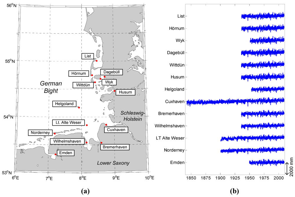
  • Monthly MSL data from tide gauges located in the southwestern North Sea (German Bight)
  • Monthly data of the station based NAO index.

2.1. Sea Level Data

This study makes use of the monthly MSL data sets of 13 tide gauges in the German Bight. The tide gauges are operated by the German Federal Waterways and Shipping Administration [23]. From the raw data (high frequency data and high and low waters), time series of MSL were reconstructed within the AMSeL project (“Mean Sea Level and Tidal Analysis at the German North Sea coastline”) [6,7]. While Wahl et al. [6,7] focused on analyzing the observed long-term changes based on annual MSL time series, in this study extended monthly MSL series are used for the first time. Figure 1 shows the investigation area of the German Bight with the location of the considered tide gauges (Figure 1a) and the monthly MSL time series of individual stations (Figure 1b). Each tide gauge provides at least 50 years of data. Although three gauges provide much longer records (Cuxhaven, Norderney and LT Alte Weser), only data from 1937 onwards are considered here to assure comparability of the results, especially from linear trend analyses.
Figure 1. Investigation area with the location of analyzed gauges (a) and the monthly MSL time series of the single records (b).
Water 04 00170 g001
The MSL data sets described above are considered in different ways with respect to the main objectives outlined in Section 1. Some of the investigations are undertaken, based on the monthly MSL time series of individual stations as presented in Figure 1; e.g., partial investigations in the seasonal cycle, the inter-annual changes of monthly MSL and sensitivities of MSL per unit NAO. At different stages of the study, so-called index time series (or ‘virtual stations’) covering larger areas in the German Bight are also considered. Virtual stations are computed from a specified number of single gauges by following the approach described by Wahl et al. [7]. In this approach, the first differences of monthly MSL time series are averaged. The resulting time series are integrated backwards by adding the previously calculated averaged first differences. Three virtual stations are used in the present study. The virtual station for Schleswig-Holstein represents the northeastern part of the German Bight. It comprises the available data from the tide gauges of List, Hörnum, Wyk, Dagebüll, Wittdün and Husum. Virtual station for Lower Saxony is constructed from the time series of the tide gauges of Cuxhaven, Bremerhaven, Wilhelmshaven, LT Alte Weser, Norderney and Emden, which are all located in the southwestern part of the German Bight. A third virtual station is constructed for the entire German Bight, including all tide gauges mentioned above (the tide gauge of Helgoland is additionally used to cover the offshore region).

2.2. NAO Data

The NAO can be described as a varying strength of two atmospheric pressure fields over the subpolar and subtropical regions of the North Atlantic. The variability of the NAO is commonly described through the NAO index. This index is derived by computing the differences between anomalies of both pressure fields. The index becomes positive if both pressure systems over the Azores and Iceland are well formed, which means the combination of a low pressure field over Iceland and a high pressure field over the Azores. Periods of positive NAO generally induce low-pressure fields over Iceland resulting in high precipitation, mild temperatures and increasing westerly winds over northern Europe [15]. A negative index means a low gradient, i.e., the deviation from the mean pressure is rather small. There are two different types of NAO indices. One well established index is the so-called station based index, computed on the data basis of two different stations between north and south. Jones et al. [24] computed an index using the difference between sea level pressure anomalies at Gibraltar and Reykjavik. One typical uncertainty of this index is that the stations are fixed in space, while the NAO centers (centers of the pressure fields—centers of action; COA) underlie movements resulting from annual cycles [25] or other processes. Therefore, the use of principle component analysis of atmospheric pressure constitutes is the more sophisticated approach. However, detailed comparison of the two different indices (not shown here) pointed out that the differences between the two indices are small and do not have influences on the results of this study (i.e., regression and trend analyses). Hence, the NAO index, established by Jones et al. [24], is used. The data set was downloaded from the website of the Climatic Research Unit, University of East Anglia [26] for the time period from 1937 to 2008.

3. Methods

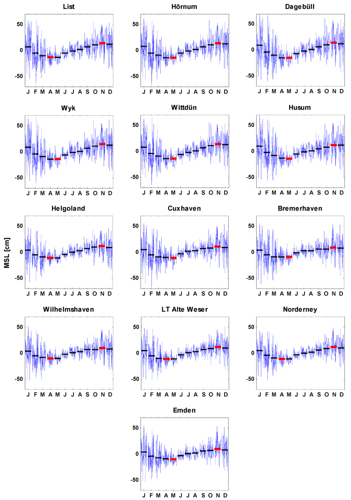
3.1. Calculating the Seasonal Cycle

At this stage, the seasonal cycle of the time span from 1951 to 2008 (all tide gauges provide data for this period) is analyzed. As a long-period tide, the seasonal cycle is formed by the solar annual (Sa) and solar semiannual (Ssa) tidal constituents with periods of 12 months and 6 months driven by solar heating [27]. There are different ways of how to compute the seasonal MSL cycle from tidal observations. An empirical method is described by Pezzulli et al. [28], in which the seasonal cycle is represented by averaging each calendar month over a defined time span. Another option is to use harmonic analysis, in which the annual cycle can be described by its amplitude and phase [29]. For the present study, the empirical description of the seasonal cycle is considered.
In a first step, the monthly MSL records are de-trended by using linear regression analysis. The removal of the linear trend enables the consideration of the annual cycle separately from its annual long-term development. In a second step the de-trended monthly MSL series are transferred into twelve time series for each calendar month (i.e., one time series for January, one for February, and so on). The annual series of each month are averaged over the time span from 1951 to 2008. These averages represent the mean seasonal cycle. The seasonal cycle is then plotted in a similar manner as presented in [30].
Furthermore, the year-to-year variability of the maximum and minimum values of the seasonal cycle is analyzed. It is calculated how often each month the maximum or minimum monthly intra-annual sea level (absolute frequency) occurs within a decade. Seven different decades, starting with 1939 to 1948 and ending with the decade 1999 to 2008, are evaluated.

3.2. Amplitudes of the Seasonal Cycle

When using the empirical description of the seasonal cycle, we define the amplitude as the difference between the maximum and minimum monthly values for the analyzed period. In this study, the inter-annual development of the amplitude of the seasonal cycle is of special interest. It is analyzed whether changes in the amplitudes of the seasonal cycle are evident from the available observations, as such changes may enhance flood risk for the investigation area. The amplitude is computed for each single year of the analyzed de-trended time series, introduced in Section 3.1. These investigations are solely done for the two virtual stations of Schleswig-Holstein and Lower Saxony.

3.3. Inter-Annual Changes in Monthly MSL

As described above, Wahl et al. [7] analyzed the long-term development of MSL, based on annual data sets. Here, the inter-annual changes in monthly MSL series of each of the 13 tide gauges along the German North Sea coastline are analyzed. One major interest for flood risk management is whether or not the MSL changes are homogeneous over the whole year or different seasons, respectively. Inhomogeneous changes in different seasons (e.g., winter and summer) may affect the phase of the seasonal cycle. Hence, the inter-annual development of winter and summer season is analyzed for each site and for different time spans. We define the winter season as the first half of the so-called “hydrological year”, which includes 6 months between November and April (hereafter: wMSL). Consequently, the summer season comprises the months from May to October of each year (hereafter: sMSL). The time spans under consideration are the same as used by Wahl et al. [7] to ensure comparability of the results of both studies. Because of the length of the different data sets three different time spans are used. The first one and the longest one considered for the present study starts in 1937 and ends in 2008. In this period three gauges (Emden, Helgoland, Wyk) cannot be taken into account because of missing data. The second time span covers the years between 1951 and 2008. For this time span all gauges can be analyzed, even if the Helgoland tide gauge starts in 1953 (more than 93% of the data of all records are available). The third time period consists of 38 years of data from 1971 to 2008. The inter-annual changes are solely analyzed with respect to their long-term linear development.

3.4. The Influence of NAO on MSL

To evaluate the relationship between inter-annual MSL variability and regional climate patterns, the monthly MSL time series of the virtual stations of Schleswig-Holstein, Lower Saxony and the entire German Bight are compared to the NAO index. In a first step, the MSL time series for each month are correlated with the analogical NAO time series. The significance of the correlation coefficients rxy is tested with a t-test as described by von Storch and Zwiers [31].
The total sea level, which is recorded by tide gauges, is composed of three main components: the astronomical tides, the MSL and the surge component [27]). The surge component is generally larger in the storm surge season during the winter. Hence, the NAO index as a proxy for westerly winds over the North Atlantic is mostly useful in the colder season of the winter months. From correlation and trend analyses (see Section 4.4) it was found that the NAO influence on MSL is largest between January and March. Hence, these months are considered for most of the analyses where the connection between NAO and MSL is investigated. The MSL values of the three months are averaged for each year to yield a time series, which is denoted here as short winter MSL (hereafter referred to swMSL and swNAO for short winter NAO). The interaction of swMSL and swNAO is analyzed with linear regression models between swMSL time series and corresponding swNAO time series following the approach proposed by Wakelin et al. [17]. In a first step, both short winter time series (i.e., swMSL and swNAO) are de-trended. Afterwards, the de-trended swMSL values are regressed with the de-trended swNAO values. Thus, the sensitivity of the swMSL to the swNAO index can be estimated, suggesting that the swMSL is a linear function of the swNAO index. Furthermore, the NAO effects are subtracted from the swMSL to estimate the influence of the swNAO on long-term changes of swMSL in the German Bight. For comparison, linear trends are computed for the original swMSL time series and the swNAO corrected swMSL time series (i.e., difference between swMSL and regression residuals).
For the detection of non-linear changes in both parameters (swMSL and swNAO), the time series are smoothed. Smoothing techniques (or low pass filters) are often applied when analyzing climatic time series, as such time series cannot be exactly described mathematically [32]. The different techniques available from literature are controversially discussed by the scientific community, because of their mathematical background and especially with respect to different techniques of computing values for the smoothed time series near the sample boundaries (see e.g., [7,33,34,35]). Here, a locally-weighted-scatterplot-smoother (LOWESS) [36,37] in combination with Monte-Carlo autoregressive padding (MCAP) as described in [6,7] is used. The MCAP method is applied to assess uncertainties when continuing smoothed time series to the end of the original time series. The LOWESS filter considers individual polynomial functions and the weighted least squares method and represents a robust low pass filter assigning lower weight to outliers. The method is applied here to detect different periods of sea level rise and fall (or non-linear changes in the NAO index) that cannot be detected through linear trend analyses. Furthermore, the smoothed time series are used to derive the rates of rise (for both MSL and NAO) by calculating the first differences.

4. Results

4.1. Seasonal Cycle of MSL

In this section the results from analyzing the seasonal component of the de-trended monthly MSL are presented. The variability of the seasonal cycle is figured by the means of month plots that are shown in Figure 2. The blue lines represent the time series for every single month over the period 1951 to 2008 (i.e., for example, all January values from 1951 to 2008). The horizontal black lines represent the average values for the particular month. The bold red lines show the months with minimum and maximum values of the seasonal cycle. For all tide gauges in the German Bight the maximum is found in November, while the minimum is in April for List, Wilhelmshaven, LT Alte Weser, Helgoland and Norderney and in May for Hörnum, Wyk, Dagebüll, Wittdün, Husum, Cuxhaven, Bremerhaven and Emden. The amplitude of the seasonal cycle is higher along the northeastern coastline (i.e., the state of Schleswig-Holstein) with values from 27–29 cm compared to the southwestern part of the German Bight (i.e., the state of Lower Saxony) with values for the amplitudes of about 20–23 cm. These amplitudes are higher than those computed for the North Atlantic region (e.g., [30]), but comparable to those for the Baltic Sea reported in [38].
The plots of the seasonal cycle in Figure 2 further show higher variability in the MSL for the winter months compared to the summer months. The seasonal cycle becomes visible at each tide gauge, but is overlapped by a large inter-annual variability. Sea levels in the North Sea are generally driven by atmospheric effects: On the one hand, atmospheric pressure fluctuations affect sea levels through the inverse barometer effect. On the other hand, cross-shore winds as well as alongshore winds together with the Coriolis effect can cause a sea level increase (or decrease) near the coastline. Generally these effects are stronger during the winter seasons when storm surges are stronger and more frequent [17]. Similar to the gradient in the seasonal amplitudes, the overall inter-annual variability is higher in the northeastern part of the German Bight (i.e., the state of Schleswig-Holstein) compared to the region of Lower Saxony in the southwestern part.
The year-to-year variability of maximum and minimum values of the seasonal cycle in the German Bight is analyzed for all of the 13 tide gauges during the last 7 decades from 1939 on (results are summarized in Figure 3). For every single decade the occurrence time of maximum and minimum values is evaluated. As it is to be expected from Figure 2 the maximum and minimum values are widely distributed over the year. Maximum values occurred between August and March with an accumulation during November and February, while minimum values are distributed over several months between October and June with an accumulation between February and May. The occurrence time of both maximum and minimum values was found to be homogeneous between the different tide gauges.
Figure 2. Plot of the annual MSL component for each gauge and the time period from 1951 to 2008. The blue line represents the monthly values for each year. The horizontal lines figure the mean value of the annual component for single months over the whole time span. The red lines figure the month where the minimum and maximum values of the annual component occur.
Water 04 00170 g002
Figure 3. Development of the occurrence time of maximum (N–F) and minimum (F–M) values of the seasonal cycle over the last seven decades between 1939 and 2008 for the two virtual stations Schleswig Holstein (left) and Lower Saxony (right).
Water 04 00170 g003
Furthermore, the evaluation of the occurrence time shows regional homogeneous change in the last two decades (i.e., 1989 to 2008) compared to the first five analyzed decades (i.e., 1939 to 1988). While in the first five decades maximum values of the seasonal cycle predominantly occurred during November and December, after 1988 the months of January and February show an increasing number of maximum values. Simultaneously, the occurrence time of minimum values shifted from February and March into April and May. This is ideally represented by the two virtual stations of Schleswig Holstein and Lower Saxony in Figure 3. The figure shows histograms of absolute frequency of maximum and minimum values for the months of accumulation (i.e., November/December and January/February for maximum values; February /March and April/May for minimum values) over the seven decades. Before 1988 in approximately 55% of all years’ maximum values occurred during November and December, while afterwards the percentage decreased to 30%. The amount of maximum values in January and February in turn increased from approximately 23% before 1988 to 50% afterwards. For the minimum values, a similar development is found. While in the first five decades the dominant months of accumulation are February and March (approximately 49%; April and May approximately 26%), in the last decades the minimum of the seasonal cycle predominantly peaks in April and May (approximately 53%; February and March approximately 25%).

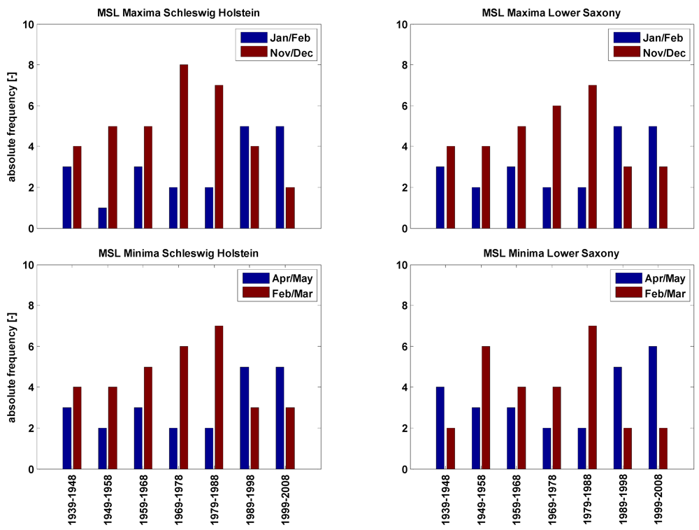
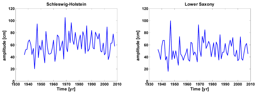
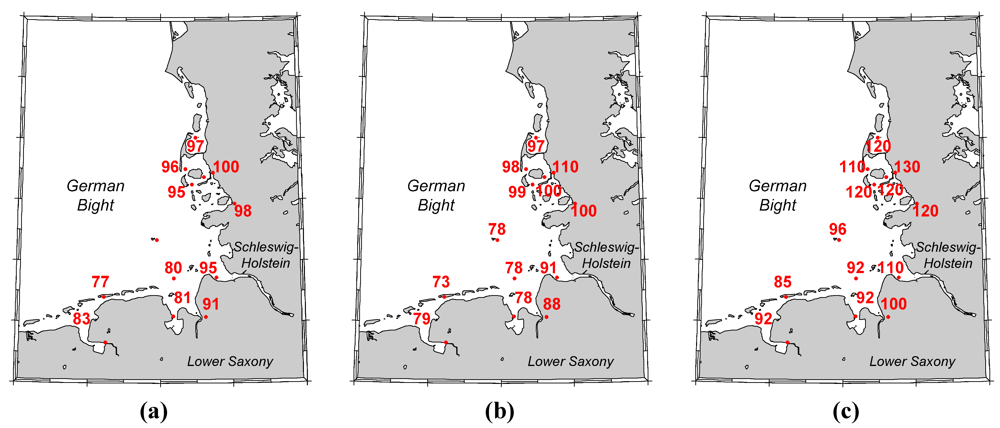
4.2. Annual Amplitudes of the Seasonal Cycle

Annual amplitudes of the seasonal cycle are computed as differences between maximum and minimum values for each year. Figure 4 shows the temporal development of the amplitude of the two virtual stations for Schleswig-Holstein and Lower Saxony and for the time period from 1937 to 2008. Both time series show similar temporal behaviors. The correlation coefficient of the amplitudes of both areas is found to be r = 0.93, whereas the amplitude of the annual cycle for Schleswig-Holstein is characterized by a slightly higher variability (and a higher mean value as already mentioned in Section 4.1) compared to Lower Saxony. Note that the annual amplitudes computed by this method are considerably higher than those mentioned in Section 4.1, where average values were considered to calculate mean amplitudes (in the order of 20 to 25 cm). Here, annual amplitudes are determined and found to be of the order of 50 to 60 cm. This is caused by the high temporal variability in the German Bight, which is described in section 4.1. However, as can be seen from Figure 4, the annual amplitudes for both virtual station time series do not show significant linear trends.
Figure 4. Time series of annual amplitude for the virtual stations of Schleswig-Holstein and Lower Saxony for the period from 1937 to 2008. The annual amplitudes are computed as differences of monthly maximum and minimum values for each year.
Water 04 00170 g004

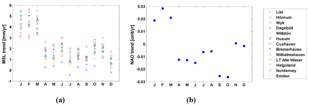
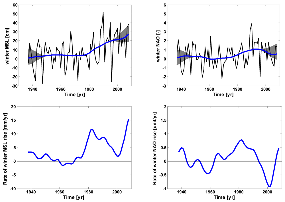
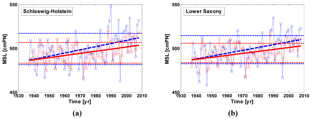
4.3. Inter-Annual MSL Changes

In this section, inter-annual MSL changes are analyzed for each tide gauge site. The time series are divided into winter (November to April, wMSL) and summer (May to October, sMSL) seasons (see Section 3.3). Table 1 shows the linear trends (with 1 − σ standard errors) for different time periods. Values are marked bold if the trends of the two seasons under consideration differ significantly, i.e., the difference between both trends is larger than the maximum standard error. The estimated trends are different in both seasons for all of the time periods and tide gauges under consideration, but statistically significant differences are only found for the two time periods from 1937 to 2008 and 1951 to 2008. Even if they also show different seasonal tendencies, the tide gauges of Husum and Emden are striking here, as their seasonal trends are not statistically significant. While in the first two time spans the winter season trends rise by a factor of up to 2.5 (on average), compared to the trends in the summer season (differences are in the order of 1.0 to 1.5 mm/yr), they are only 1.1 times (on average) higher (differences in the order of 0.5 mm/yr) for the shorter time period from 1971 to 2008. Similar to the findings reported by Wahl et al. [7], highest trends are detected for the shortest period from 1971 to 2008. While the trends for the wMSL and sMSL of the first period from 1937 to 2008 are about 2.4 mm/yr and 1.6 mm/yr respectively (averaged over all sites), the trends for the last period (i.e., 1971 to 2008) are about 3.9 mm/yr and 3.4 mm/yr for the two seasons. Standard errors increase inversely to the length of the time period under consideration. Thus, smallest standard errors (in the order of 0.5 mm/yr and 0.3 mm/yr for the wMSL and sMSL, respectively) are found for the first period (i.e., 1937 to 2008). The highest standard errors, in the order of about 1.31 mm/yr and 0.64 mm/yr, are derived for the final period (i.e., 1971 to 2008). Furthermore, averaged standard errors (over all gauges) show significant differences between wMSL and sMSL.
Table 1. Linear trends for different common periods differentiated in winter (N–A) and summer season (M–O). The values are marked in bold if trends of the two considered seasons differ significantly.
Tide gaugeLinear trends of Regional Mean Sea Level (RMSL) for different time spans ± 1 − σ standard errors [mm/yr] differentiated in winter and summer months
1937–20081951–20081971–2008
WinterSummerWinterSummerWinterSummer
List2.5 ± 0.51.5 ± 0.33.3 ± 0.61.5 ± 0.44.6 ± 1.33.8 ± 0.7
Hörnum2.8 ± 0.51.7 ± 0.33.6 ± 0.71.8 ± 0.44.6 ± 1.33.9 ± 0.7
Wyk -- -- 3.9 ± 0.71.8 ± 0.45.1 ± 1.44.3 ± 0.6
Dagebüll 2.3 ± 0.5 1.2 ± 0.3 3.1 ± 0.7 1.3 ± 0.4 4.0 ± 1.43.5 ± 0.8
Wittdün2.9 ± 0.51.8 ± 0.33.3 ± 0.71.9 ± 0.44.0 ± 1.43.8 ± 0.7
Husum2.3 ± 0.52.0 ± 0.32.8 ± 0.72.1 ± 0.43.6 ± 1.53.7 ± 0.7
Helgoland -- -- 2.9 ± 0.6*1.3 ± 0.4*4.0 ± 1.23.4 ± 0.6
Cuxhaven2.7 ± 0.51.5 ± 0.32.7 ± 0.71.2 ± 0.43.9 ± 1.43.5 ± 0.6
Bremerhaven1.7 ± 0.50.7 ± 0.31.8 ± 0.70.2 ± 0.43.1 ± 1.41.9 ± 0.6
Wilhelmshaven2.3 ± 0.41.4 ± 0.22.7 ± 0.61.3 ± 0.33.8 ± 1.23.1 ± 0.6
LT Alte Weser2.0 ± 0.41.4 ± 0.32.2 ± 0.61.2 ± 0.43.3 ± 1.22.9 ± 0.6
Norderney2.8 ± 0.41.9 ± 0.23.4 ± 0.62.2 ± 0.34.3 ± 1.14.2 ± 0.5
Emden-- -- 1.8 ± 0.60.9 ± 0.32.2 ± 1.22.0 ± 0.6
* Some years of the time period under consideration are missing, but at least 93% are available.
As outlined by Wahl et al. [7], from analyzing annual MSL time series, higher trends are found for tide gauges along the coastline of Schleswig-Holstein compared to Lower Saxony.

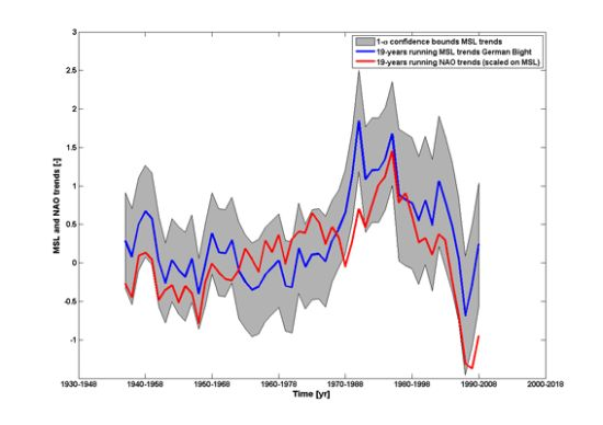
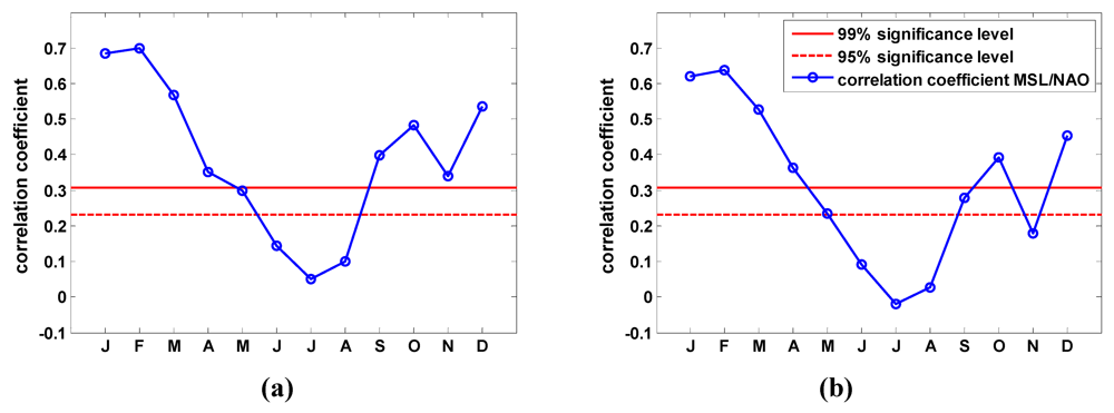
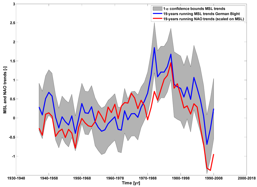
4.4. Relationship between NAO and MSL

The relationship between the de-trended MSL, represented by the two virtual stations for Schleswig-Holstein and Lower Saxony, and the de-trended NAO is shown in Figure 5. The blue line represents the correlation coefficients for the individual months and the period from 1937 to 2008. The red lines indicate the 95% and 99%-significance levels (based on t-test statistics (e.g., [31])). There is a strong annual cycle in the correlation, with significant correlations in the winter season and weak or no correlations in the summer months. For the whole year, correlation coefficients for time series from Schleswig-Holstein and the NAO are slightly higher than the coefficients for MSL time series from Lower Saxony and the NAO. This gradient between Schleswig-Holstein and Lower Saxony has also been found in the variability of the seasonal cycle in Sections 4.1 and 4.2. The highest correlations are found from January to March. This leads to the assumption that the highest influence of NAO on long‑term development of MSL should also be found in these three months. While for the correlation analysis only de-trended time series are investigated, it is of particular importance in which manner the NAO may influence linear trends of MSL. To consider this, linear trends of MSL time series for each month are compared with those found from corresponding monthly NAO time series. The linear trends of monthly time series for both parameters are pictured in Figure 6. At the top of the figure the different dots indicate the trends of monthly MSL time series for the individual sites and the period from 1951 to 2008. Figure 6 (bottom) shows the monthly trends of the NAO. Both parameters show similar behavior for the winter months, indicating significantly higher trends from January to March compared to the remaining months (i.e., significantly different on the 1σ-significance level). Although correlation over the whole year is not constant between the two parameters and partially weak (especially in the summer months), a similar trend pattern is notable from Figure 6. This behavior was also found for the other two time periods (i.e., 1937–2008 and 1971–2008), which are not pictured here.
Figure 5. Correlation coefficients between NAO and MSL for the period 1937–2008. (a) shows the relationship for the virtual station ‘Schleswig Holstein’; (b) shows the relationship for the virtual station ‘Lower Saxony’. The thicker horizontal red lines show two significance levels by using a t-test.
Water 04 00170 g005
The similar trend pattern, with higher values for the three months from January to March, leads to the assumption that the high NAO trends in the three winter months strongly influence the MSL changes for the same months. Hence, the interaction between swMSL and swNAO is described by the sensitivity of swMSL (unit is mm) per unit swNAO. As described in Section 3.4, sensitivity is estimated by applying linear regression models between both parameters. Figure 7 shows the derived sensitivities for the three different time periods that have been used in Section 4.3 for the linear trend analyses. The largest sensitivities of the swMSL are found at the northeastern coastline in the area of Schleswig-Holstein with values up to 130 mm per unit swNAO index for the last period (i.e., 1971 to 2008), while the sensitivities for the area of Lower Saxony are considerably smaller (up to 45 mm per unit swNAO).
Figure 6. Inter-annual trends of monthly MSL (a) and monthly NAO (b) for the period from 1951 to 2008.
Water 04 00170 g006
Figure 7. Sensitivity (sea level changes in mm/unit NAO change) of swMSL (January to March) to swNAO for different time spans (1937–2008 (a); 1951–2008 (b); 1971–2008 (c)) and different tide gauges.
Water 04 00170 g007
The sensitivities change over time. While the sensitivity is almost the same for the first two periods (1937 to 2008 and 1951 to 2008), it is considerably higher for the last period (1971 to 2008). Jevrejeva et al. [20] also reported a remarkable temporal change of the NAO influence on sea levels in Northern Europe, with highest correlation values between both parameters found for the last three decades. These results indicate that the NAO influences the inter-annual variability of winter MSL at least to some degree. In agreement to the results presented by Jevrejeva et al. [20], the contribution of the NAO is 30–35% of winter MSL variability in the German Bight. Generally, MSL is higher in winters with positive NAO indices than in winters with negative NAO indices.
If the swNAO influences the swMSL variability in the German Bight over a specified time period and shows a significant trend at the same time, the question arises whether the swNAO also influences the swMSL long-term trends as well. Tsimplis et al. [21] analyzed the NAO influence on long-term winter (December to March) MSL trends for different gauges in Northern Europe and found that in most cases the MSL trends are smaller if the NAO influence is considered (of course only for those gauges where a positive correlation exists between NAO and MSL). To investigate the swNAO influence on long-term swMSL trends in the German Bight, Table 2 shows trends calculated directly from the swMSL time series (January to March) and for comparison, the trends, which are found after the swMSL time series, are corrected for the swNAO influence. The latter is estimated by applying the same linear regression models that have been used to study the sensitivities as shown in Figure 7. Beside the two virtual station time series for Schleswig-Holstein and Lower Saxony, a virtual station for the entire German Bight is also considered at this stage. The results clearly point out that the swNAO influences the long-term winter MSL trends. Again, however, this influence changes over time. Considering the first two time spans from 1937 to 2008 and 1951 to 2008 the winter MSL trends are about 3.3 mm/yr and 4.3 mm/yr, respectively (for the entire German Bight). After removing the swNAO influence the residuals show smaller trends of 2.2 mm/yr and 2.3mm/yr. The trends for the two virtual stations Schleswig-Holstein and Lower Saxony show small differences with a higher swNAO influence in Schleswig-Holstein than in Lower Saxony as was expected from the results presented in Figure 5. As reported in Section 4.3, the wMSL trends increase for the shorter time period from 1971 to 2008. For the virtual station of the entire German Bight, the swMSL trend is found to be 7.6 mm/yr, whereas it decreases to 6.2 mm/yr after removing the swNAO influence (equals a trend reduction of 18%). Due to the reduction of the variability by considering the swNAO influence, the standard errors of the estimated trends also decrease (from 2.4 mm/yr to 1.4 mm/yr).
Table 2. Linear trends for the swMSL of three synthetic tide gauges before and after swNAO correction (trends which change significantly after removing the NAO influence are marked bold).
Tide gaugeLinear trends of RMSL for different time spans ± 1 − σ standard errors [mm/yr] differentiated in winter (J–M) RMSL and NAO corrected winter (J-M) RMSL (correlation NAO/MSL)
1937–2008 trend1951–2008 trend1971–2008 trend
with NAOwithout NAOwith NAOwithout NAOwith NAOwithout NAO
German Bight3.3± 0.9 (0.75)2.2 ± 0.64.3 ± 1.2 (0.75)2.3 ± 0.87.6 ± 2.4 (0.77)6.2 ± 1.4
Schleswig Holstein3.6 ± 0.9 (0.76)2.4 ± 0.65.0 ± 1.1 (0.76)2.7 ± 0.98.4 ± 2.6 (0.78)6.8 ± 1.5
Lower Saxony3.2 ± 0.8 (0.73)2.2 ± 0.63.7 ± 1.1 (0.73)1.9 ± 0.86.9 ± 2.2 (0.75)5.6 ± 1.3
To analyze more in detail in which way the swNAO influences decadal swMSL trends, 19-year running linear trends of swMSL (for the entire German Bight) and the swNAO are shown in Figure 8. According to their different scaling, the 19-year running swNAO trends (red line) are scaled to be comparable to the 19-year running swMSL trends. The latter are represented by the blue line and corresponding 1 − σ standard errors (grey-filled areas) are also shown. Both time series of the running 19-year linear trends show a similar temporal behavior with only two phases (1971 to 1989 and 1972 to 1990, 1989 to 2007 and 1990 to 2008), where the swNAO trends proceed outside the 1 − σ confidence intervals calculated for the swMSL trends. More than 93% of all estimated swNAO trends proceed inside the 1 − σ confidence intervals of the swMSL trends.
Figure 8. 19-year running linear trends of swMSL (blue line) at the virtual station German Bight and swNAO (red line) for the period from 1937 to 2008. The grey-filled area indicates the 1 − σ confidence bounds for the linear trends estimated by linear regression.
Water 04 00170 g008
Figure 9 shows the time series of the swMSL for the entire German Bight (top, left, black line) and the swNAO index (top, right, black line) for the period from 1937 to 2008 and the smoothed time series (blue lines in the upper subplots). The rates of rise calculated as the first differences from the smoothed time series are shown in the lower subplots of Figure 9. The window length for smoothing the time series was chosen to be 30 years and the values near the sample boundaries result from applying the MCAP method briefly described in the Section 3 and in [6]. The uncertainties resulting from smoothing the time series to the boundaries are represented by the grey-shaded areas. The time series of the swNAO and swMSL are highly correlated (r = 0.74). Both of the original time series show similar peak values in many years: e.g., 1938, 1941, 1947, 1967, 1983, 1990, 1996 and 2002. In some years the values are also different, suggesting that the NAO is not the only driver of MSL variability. However, the smoothed time series show a similar temporal behavior (especially between the mid 1970’s and mid 1990’s) with some differences near the sample boundaries. By considering the rates of rise (Figure 8, bottom) both time series show similar tendencies near the sample boundaries as well, even if the estimates for the boundaries are uncertain. Although the rates of rise indicate negative values for the swNAO index and positive values for the swMSL at the end of the 1990’s, they are marked by a comparable shape. Hence, significant influences of the swNAO on swMSL can be detected. These influences changed over time, suggesting the non-stationary behavior of the COA’s of the NAO as is described by Kolker and Hameed [39]. In some phases it seems that other external forcing factors are getting stronger from time to time. The phases in the beginning of the 1960’s and the last ten years are striking here.
Figure 9. Time series of swMSL and swNAO for the German Bight (black lines, top) and LOWESS smoothing (blue lines, top). The grey-filled areas indicate the results of the MCAP method. The annual rates of rise calculated as the first differences of the smoothed time series are shown in the plots at the bottom.
Water 04 00170 g009

4. Discussion

Recent assessments of MSL changes in the German Bight have mostly focused on inter-annual changes and hence considered annual time series. Especially for aspects of coastal safety management, inter-annual MSL assessment is particularly important as it considerably affects storm surge heights and frequencies. As pointed out in [40] and [41], accelerating MSL diminishes the present safety level along the German North Sea coastline, even if the vulnerability is relatively moderate. However, increasing sea levels involve a higher water inflow in the event of the failure of coastal protection structures. Storm surges are the main events affecting coastal areas, especially when they are combined with high astronomical tides (e.g., spring tides). Changes in the seasonal cycle may influence water levels occurring during a storm surge season and until now seasonal investigations of MSL in the German Bight have not received much attention.
The results from analyzing the intra-annual variability in MSL along the German North Sea coastline (Section 4.1) show that there are considerable seasonal effects. As a shallow shelf sea, the North Sea is strongly influenced by wind forces. This implies higher variability of MSL in the storm surge or winter season respectively, compared to the summer season. In summer months the wind stress is considerably lower, which results in lower variability. Therefore, tidal forces have a stronger relative influence on the MSL. Furthermore, the results point to some differences along the coastline with higher variability in the northeastern than in the southwestern part of the German Bight. These differences result from the fact that westerly winds are predominant in the North Sea with a stronger influence on the coastline of Schleswig-Holstein with its north-south expansion.
The mean amplitude of the seasonal cycle in the German Bight, computed by the empirical approach, is found to be about 27 to 29 cm for the area of Schleswig-Holstein and about 20 to 23 cm for tide gauges located in Lower Saxony. The amplitude is considerably higher than in other parts of the world. Generally, in mid latitudes the mean amplitude of the seasonal cycle is about approximately 4 to 7 cm [27]. In the German Bight the seasonal cycle is overlapped by strong variability, resulting from wind forces, effects from river run-off, salinity and thermal effects. The averages of the MSL values for the particular months and over the period from 1937 to 2008 illustrate that the seasonal cycle reaches its maximum in November, while the minimum occurs in April or May. The strong variability leads to a strong year-to-year variation of maximum and minimum values. Maximum values scatter over 8 months (from August to March) and minimum values have been found between October and June, even if there are considerable accumulations. The decadal analysis of the maximum and minimum values points to a shift of these accumulations. The maximum values have been moved over the last two decades from November/December to January/February and the minimum values have been shifted from February/March to April/May. As described above, there is a large amount of inter-annual variability in the phase of the seasonal cycle. Changes in the phase of the seasonal cycle have been repeatedly observed in different climatic parameters (e.g., [42,43]), but the causes are poorly understood [44]. The changes in phase are consistent between stations but, probably due to the large natural variability, are statistically insignificant. However, similar studies support such changes. First of all, similar findings for the maximum values of the seasonal sea level cycle in the Baltic Sea were presented by Johansson et al. [42]. The relationship between the seasonal cycles of NAO and MSL were analyzed by Yan et al. [19]. They compared anomalous strong (and weak) signals in both parameters. In their Figure 7 they computed the seasonal cycles before and after 1989. This figure shows that the seasonal NAO cycle after 1989 peaks in the months of January/February, while before it rather peaks in autumn. If—as expected here—the NAO or NAO-related processes drive changes in the phase of the seasonal MSL cycle, the observed changes are a result of an anomalous strong NAO cycle after 1988. Apart from this, Marcos and Tsimplis [45] also found higher trends in MSL for the winter season (December to March) and the period from 1960 to 2000 for tide gauges located in the German Bight, by analyzing the output of a two-dimensional hydrodynamic model of the NW European shelf. The authors argue that approximately 4 mm/yr (i.e., about 50%) of the estimated trend is due to meteorological forces. Furthermore, Lehmann et al. [43] studied the variability of different climate related parameters, such as wind speed or precipitation in comparison to the NAO for the greater Baltic Sea area (including the southeastern parts of the German Bight) over a period from 1958 to 2009. They report a seasonal shift of strong winds from autumn to winter and early spring in line with an eastward shift of the atmospheric COA. Since wind in particular is the major factor in local sea level variability in the North Sea [17], the observed phase shift in sea level can be explained (at least to some degree).
Another challenge regarding the high variability in the German Bight is that the computation of the year-to-year amplitude of the seasonal cycle becomes non-stationary with respect to its phase (see Section 4.2). Hence, using maximum and minimum values to calculate annual amplitudes results in a comparison of values derived from different monthly values in particular years. This means that the computation of amplitude is strongly biased by other effects, such as variability caused by local meteorological influences, river run-off or thermal effects. Different methods to separate the annual cycle from the overlapping variability can be found in the literature. On the one hand, variability can be filtered out by investigating seasonal averages. Hünicke et al. [38] computed the year-to-year amplitude by using seasonally-averaged maximum and minimum values (winter: November to January; spring: March to May). This leads to a better approximation of the intra-annual amplitude. On the other hand, moving monthly averages of several years or moving Fourier analysis may be used, as described by Plag and Tsimplis [29] and Ekman [46]. Furthermore, one of the reviewers proposed inter-quartile ranges for the computation of annual amplitudes. This method is more robust against outliers. For the present study, all of these approaches have been tested in addition to the min/max-approach described in Section 3.1 in order to analyze whether there are any long-term changes evident in the amplitudes of the seasonal cycle. Amplitudes, computed by the min/max-approach, lead to values of approximatly 50–60 cm on average, compared with much smaller values derived using the other approaches. However, the aim was to calculate any long-term changes in the annual amplitudes. From all the different methods, no significant trends in the amplitude of the seasonal cycle could be found in the German Bight.
The detailed analysis of long-term changes in seasonal MSL components (Section 4.3) indicates that the long-term trends in the wMSL are higher than in the sMSL for all time periods under consideration (i.e., 1937 to 2008, 1951 to 2008 and 1971 to 2008), but only statistically significant for the first two periods. It has been noticed that the differences in the long-term changes of the two seasons are unsteady over time. While in the first two time spans (i.e., 1937 to 2008 and 1951 to 2008) the winter trends are more than two times stronger (on average) than the summer trends, they are more equal for the short time period from 1971–2008. From analyzing the trends for each single month of a year (see Section 4.4), considerably stronger MSL trends are found for the months from January to March. The estimated trends are in agreement with those presented for the North Sea area in [46] and potentially caused the shift in the maximum values of the seasonal cycle described in Section 4.1. This raises the question of which parameters are the main factors causing such changes.
Due to its location on the northwestern continental shelf, the German Bight is strongly affected by meteorological forces. Therefore it is assumed that changes in the NAO are linked to changes in the seasonal cycle of the MSL. The MSL shows significant correlations with the NAO in the winter months, especially from January to March, whereby the influence is not stationary in time as described by Yan et al. [19] and Jevrejeva et al. [20]. However, the higher trends between January and March are also imaged in the monthly NAO values. This indicates that the swNAO is one major driving factor for changes in swMSL, which results in the increasing gradient between winter and summer season and the shift in the phase of the seasonal cycle. The smaller gradient between the MSL in the summer and winter half year after 1971 compared to the two longer time periods is most likely due to lower trends in the swNAO for this time period. From separate trend analyses (not discussed in detail here) it was depicted that the swNAO shows similar tendencies for all of the three considered time periods, but the smallest trend is calculated for the 1971–2008 period. Hence, the acceleration in swMSL after 1971 cannot be explained solely by higher trends in the swNAO index over the same time period, particularly with regard to the strongly increasing trends in summer season observed in section 4.3.
The interaction between swNAO and swMSL is considered by computing sensitivities of swMSL (in mm) per unit swNAO (see Section 3.4 and Section 4.4). The identified sensitivities are comparable to those found in other studies for the same area. Wakelin et al. [17] and Tsimplis et al. [21] reported sensitivities of up to 96 mm/unit NAO (December to March) in the German Bight using a two dimensional tide + surge model for the time period from 1955 to 2000. Tsimplis et al. [21] pointed out that the sensitivity of model data was found to be lower compared to the sensitivity computed with tide gauge data. They suggested an additional sea level influence of the NAO through thermosteric effects or model inaccuracies. Tsimplis et al. [47] confirmed sensitivities in the order of 10 mm/unit NAO via thermosteric effects. Nevertheless, the sensitivities computed in this study show that the results from the above-mentioned studies are still valid for time periods covering nearly three more decades than the model data. The spatial distribution of the sensitivity in the German Bight is not homogeneous with stronger sensitivity (up to 130 mm/unit swNAO) in the northeastern part compared to the southwestern part (up to 110 mm/unit swNAO). This gradient becomes logical, comparing the computed sensitivities with the results of the two dimensional tide + surge model presented in [17,18,21]. This is confirmed by the correlation analyses and supports the assumption that westerly winds are responsible for higher variability along the coastline of Schleswig-Holstein.
We also analyze the influence of swNAO on long-term swMSL changes. The results, given in Table 2, indicate that the swNAO influences swMSL, in two different ways. On the one hand, the swNAO influence explains 30–35% of the inter-annual swMSL variability in the German Bight. These findings are in agreement with the results presented by Jevrejeva et al. [20] for the North and Baltic Sea, even if the inverse barometric effect has not been considered for the present study. On the other hand, the swNAO also influences the long-term swMSL trends in the German Bight. For all of the three time periods under consideration, the NAO influence leads to higher trends from January to March. For the first two time spans (i.e., 1937 to 2008 and 1951 to 2008) the swNAO explains up to 47% (2.3 mm/yr) of the estimated swMSL trends. For the period from 1971 to 2008, the swNAO influence is considerably smaller and explains about 18% (1.3 mm/yr) of the estimated swMSL trend. This is caused by a smaller trend in the swNAO for the latter time period compared to the longer periods considered in the present study. This highlights that the influence of the swNAO on long-term swMSL trends depends on the time period under consideration. This is also confirmed from analyzing 19-year running linear trends and the non-linear behavior for the time period from 1937 to 2008. The main influences of the swNAO on swMSL in the German Bight are summarized in Figure 10. The swMSL estimations for Schleswig-Holstein (Figure 10a) and Lower Saxony (Figure 10b) are shown before (blue line) and after, removing the swNAO influence (red line) (only the long time period from 1937–2008 is considered). The standard deviations are represented by the dotted lines and the long-term trends are highlighted as bold lines. For both virtual stations it can be stated that a correction of the swMSL estimations for the swNAO influence causes a reduction of variability and trends.
The results presented here aim to clarify the role of meteorological forces on swMSL in the German Bight. The different behavior of MSL during the months from January to March (compared to the remaining months) led to a redistribution of annual maximum peaks in the last two decades. Assuming that this shift consolidates, the future flood risk may be affected more intensively than previously expected. As described by Pugh [27], highest storm surges can be observed when they are accompanies by high astronomical tides and high MSL values. Hence, higher wMSL/swMSL may affect coastal structures in two different ways. First, higher wMSL/swMSL causes higher constant loads due to extended duration times of high water levels. Second, the maximum water level heights during storm surge events may be also affected. Since the NAO is one of several important driving factors for wMSL/swMSL, it will be crucial in which direction the NAO will develop in future. It is well known that a significant trend to more positive values in the NAO index has been observed over the last decades of the 20th century (especially between the 1960’s and 1990’s). This has caused a warmer and more humid climate over Northern Europe [15], but it is rather uncertain how the NAO will change in future. Different global climate models have been used to simulate the NAO variability. The IPCC [48] exposed that many climate model simulations show a decrease of the arctic sea level pressure for the 21st century, which would result in more positive values of the NAO index [49,50].
Figure 10. Influence of swNAO on swMSL (1937–2008) in the German Bight. The thin lines represent the swMSL data (blue = including swNAO; red = after removing swNAO). The thin dotted lines represent the standard deviations and the thick lines show the linear trends. (a) Schleswig-Holstein; (b) Lower Saxony.
Water 04 00170 g010

5. Conclusions

MSL records from 13 tide gauges in the German Bight have been analyzed to determine the seasonal and inter-annual development of monthly MSL in the 20th and the beginning of the 21st century. The results of this study show that the seasonal cycle has mean amplitude of approximately 20–29 cm along the German North Sea coastline with minimum values in April and May and maximum values in November. The seasonal cycle is overlapped by a strong year-to-year variability, which is significantly higher during the storm surge season (October to March) than in the remaining months. The analysis of the development of the seasonal cycle in the German Bight indicates no long-term changes in the amplitude and phase but a large inter-annual variability. While between 1939 and 1988 the seasonal MSL cycle mostly peaked in November and December, in the last two decades tendencies to a stronger incidence in January and February have been observed.
The more frequent maximum values in January and February coincide with an inhomogeneous seasonal trend development in the German Bight. Considerable differences have been found between winter and summer seasons (i.e., wMSL and sMSL). For two of three analyzed periods (1937 to 2008, 1951 to 2008) wMSL is significantly higher compared to the sMSL. This gradient between summer and winter months is also found for the period from 1971 to 2008 whereas the gradient is considerably smaller and not statistically significant. The investigation of the monthly components reveals the months between January and March, which are represented in the swMSL, as the main driver of this gradient. The stronger trend in the last three decades reported by Wahl et al. [7] is confirmed in this study for both seasons. An explanation for the increasing sMSL cannot be given in this study, but will be part of future studies.
It is well known that atmospheric circulation has a considerable influence on climate variability over Northern Europe [10,11,25,43]. Since sea level responds to different climatic forces, such as wind, pressure or precipitation, the NAO becomes a reasonable proxy for such influences. Confirming earlier studies from [22,40,42,47,48], the statistical comparison of MSL and NAO shows positive correlations at tide gauges located in the German Bight. These correlations are significant in winter and autumn and weaken or get insignificant throughout the summer months. Therefore, the comparison of MSL and the NAO is only straightforward for the winter and autumn months (e.g., [22]). From the regression analysis between swMSL and swNAO it has been found that the swNAO influences swMSL in two different ways. On the one hand the swNAO explains 30–35% of the year-to-year variability of swMSL, which confirms earlier findings from Wakelin et al. and Jevrejeva et al. [17,20] for the larger North and Baltic Sea area. On the other hand similarities are found in the trend patterns of both parameters. The comparison of 19-year running trends and the rates of rise shows strong coherency between swMSL and swNAO. This is why we suggest meteorological forces as the main driving factors of swMSL changes and therefore for changes in the seasonal cycle in the past 70 years. Our results confirm the importance of seasonal sea level analysis for the matters of coastal defense strategies highlighted by previous studies for the North Sea [17,21]. In particular, in the German Bight there is a huge amount of non-tidal variability which considerably influences flood risk. Furthermore, this high degree of variability complicates reliable estimations of trends and possible future sea level developments. It can be concluded that the trend of the MSL in the German Bright is overestimated if the influences of the atmosphere are not excluded from the MSL time-series. This is important: one way to find numbers for regional future states (e.g., for the year 2100) of MSL is the comparison of the regional with the global MSL, for which projections already exist. Higher MSLs contain higher levels upon which storm surges built [51]. Hence, especially higher trends during the storm surge season are very important as they may affect the effects of storm surges along the coastline. For the future it will be important to assess the contribution of local or remote meteorological factors affecting residual fluctuations (especially on trends) which cannot be explained with the NAO index, especially for the remaining seasons (i.e., spring and summer), which have not been considered in this or related studies.

Acknowledgments

This study is part of the KLIWAS research program. KLIWAS is a departmental program initiated and funded by the German Federal Ministry of Transport, Building and Urban Development (BMVBS). We are grateful for the helpful comments of the two anonymous reviewers on a former version of the manuscript. While preparing the manuscript for this paper we benefited from technical discussion with Ivan Haigh. Furthermore, we highly acknowledge Andre Stettner-Davis for his useful English corrections.

References

  1. Church, J.A.; Woodworth, P.L.; Arup, T.; Wilson, W.S. Understanding Sea-Level Rise and Variability, 1st ed; Wiley-Blackwell: Chichester, UK, 2010; pp. 402–419. [Google Scholar]
  2. Church, J.A.; White, N.J.; Aarup, T.; Wilson, W.S.; Woodworth, P.L.; Domingues, C.M.; Hunter, J.R.; Lambeck, K. Understanding global sea levels: Past present and future. Sustain. Sci. 2008, 3, 9–22. [Google Scholar] [CrossRef] [Green Version]
  3. Bindoff, N.L.; Willebrand, J.; Artale, V.; Cazenave, A.; Gregory, J.; Gulev, S.; Hanawa, K.; Le Quéré, C.; Levitus, S.; Nojiri, Y.; et al. Observations: Oceanic climate change and sea level. In Climate Change 2007: The Physical Science Basis. Contribution of Working Group I to the Fourth Assessment Report of the Intergovernmental Panel on Climate Change; Solomon, S., Qin, D., Manning, M., Chen, Z., Marquis, M., Averyt, K.B., Tignor, M., Miller, H.L., Eds.; Cambridge University Press: Cambridge, UK; New York, NY, USA, 2007; pp. 385–428. [Google Scholar]
  4. Führböter, A.; Jensen, J. Säkularänderungen der mittleren Tidewasserstände in der Deutschen Bucht. Die Küste 1985, 42, 78–100. [Google Scholar]
  5. Jensen, J.; Mudersbach, C. Zeitliche Änderungen in den Wasserstandszeitreihen an den deutschen Küsten. In Berichte zu Deutschen Landeskunde, Themenheft: Küstenszenarien; Glaser, R., Schenk, W., Voigt, J., Wießner, R., Zepp, H., Wardenga, U., Eds.; Selbstverlag Deutsche Akademie für Landeskunde E.V.: Leipzig, Germany, 2007; pp. 99–112, Band 81, Heft 2. [Google Scholar]
  6. Wahl, T.; Jensen, J.; Frank, T. On analysing sea level rise in the German Bight since 1844. Nat. Hazards Earth Syst. Sci. 2010, 10, 171–179. [Google Scholar] [CrossRef]
  7. Wahl, T.; Jensen, J.; Frank, T.; Haigh, I.D. Improved estimates of mean sea level changes in the German Bight over the last 166 years. Ocean Dyn. 2011, 5, 701–715. [Google Scholar]
  8. Jensen, J.; Mügge, H.E.; Schönfeld, W. Analyse der Wasserstandsentwicklung und Tidedynamik in der Deutschen Bucht. Die Küste 1992, 53, 212–275. [Google Scholar]
  9. Woolf, D.; Tsimplis, M. The influence of the North Atlantic Oscillation on sea level in the Mediterranean and the Black Sea derived from satellite altimetry. In Proceedings of the Second International Conference on Oceanography of the Eastern Mediterranean and Black Sea: Similarities and Differences of Two Inter-connected Basins, Ankara, Turkey, 14–18 October 2002; pp. 145–150.
  10. Hurrell, J.W. Decadal trends in the North Atlantic Oscillation: Regional temperatures and precipitation. Science 1995, 269, 676–679. [Google Scholar]
  11. Hurrell, J.W.; Kushnir, Y.; Visbeck, M.; Ottersen, G. An overview of the North Atlantic Oscillation. In Proceedings of the EGS-AGU-EUG Joint Assembly, Nice, France, 6–11 April 2003; Hurrell, J.W., Kushnir, Y., Ottersen, G., Visbeck, M., Eds.; 134, pp. 1–35.
  12. Thompson, D.W.J.; Wallace, J.M. The Arctic Oscillation signature in the wintertime geopotential height and temperature fields. Geophys. Res. Lett. 1998, 9, 1297–1300. [Google Scholar]
  13. Ambaum, M.H.P.; Hoskins, B.J.; Stephenson, D.B. Artic Oscillation or North Atlantic Oscillation? J. Clim. 2001, 14, 3496–3507. [Google Scholar]
  14. Martin, M.L.; Valero, F.; Pascual, A.; Morata, A.; Luna, M.Y. Springtime connections between the large-scale sea-level pressure fields and gust wind speed over Iberia and the Balearics. Nat. Hazards Earth Syst. Sci. 2011, 11, 191–203. [Google Scholar] [CrossRef]
  15. Hilmer, M.; Jung, T. Evidence of a recent change in the link between the North Atlantic Oscillation and Arctic ice transport. Geophys. Res. Lett. 2000, 7, 989–992. [Google Scholar] [CrossRef]
  16. Petrow, T.; Zimmer, J.; Merz, B. Changes in the flood hazard in Germany through changing frequency and persistence of circulation patterns. Nat. Hazards Earth Syst. Sci. 2009, 9, 1409–1423. [Google Scholar] [CrossRef]
  17. Wakelin, S.L.; Woodworth, P.L.; Flather, R.A.; Williams, J.A. Sea-level dependence on the NAO over the NW European continental shelf. Geophys. Res. Lett. 2003, 7, 56:1–56:4. [Google Scholar]
  18. Woodworth, P.L.; Flather, R.A.; Williams, J.A.; Wakelin, S.L.; Jevrejeva, S. The dependence of UK extreme sea levels and storm surges on the North Atlantic Oscillation. Cont. Shelf Res. 2007, 27, 935–946. [Google Scholar] [CrossRef]
  19. Yan, Z.; Tsimplis, M.N.; Woolf, D. Analysis of the relationship between the North Atlantic Oscillation and sea level changes in Northwest Europe. Int. J. Climatol. 2004, 24, 743–758. [Google Scholar] [CrossRef]
  20. Jevrejeva, S.; Moore, J.C.; Woodworth, P.L.; Grinsted, A. Influence of large-scale atmospheric circulation on European sea level: Results based on the wavelet transform method. Tellus 2005, 57A, 183–193. [Google Scholar]
  21. Tsimplis, M.N.; Woolf, D.K.; Osborn, T.J.; Wakelin, S.; Wolf, J.; Flather, R.; Shaw, A.G.P.; Woodworth, P.L.; Challenor, P.; Blackmen, D.; et al. Towards a vulnerability assessment of the UK and Northern European coasts; the role of regional climate variability. Philos. Trans. R. Soc. A 2005, 363, 1329–1358. [Google Scholar] [CrossRef]
  22. Tsimplis, M.N.; Shaw, A.G.P. The forcing of mean sea level variability around Europe. Glob. Planet. Change 2008, 63, 196–202. [Google Scholar] [CrossRef]
  23. German Federal Waterways and Shipping Administration. Available online: http://www.wsv.de (accessed on 23 February 2012).
  24. Jones, P.D.; Jonsson, T.; Wheeler, D. Extension to the North Atlantic Oscillation using early instrumental pressure observations from Gibraltar and south-west Iceland. Int. J. Climatol. 1997, 17, 1433–1450. [Google Scholar] [CrossRef]
  25. Climate Research Unit, University of East Anglia, Norwich, UK. Available online: http://www.cru.uea.ac.uk (accessed on 23 February 2012).
  26. Hurrell, J.W.; Deser, C. North Atlantic climate variability: The role of the North Atlantic Oscillation. J. Mar. Syst. 2009, 78, 28–41. [Google Scholar] [CrossRef]
  27. Pugh, D. Changing Sea Levels. Effects of Tides, Weather and Climate, 1st ed; Cambridge University Press: Cambridge, UK, 2004; pp. 1–48. [Google Scholar]
  28. Pezzulli, S.; Stephenson, D.B.; Hannachi, A. The variability of seasonality. J. Clim. 2005, 18, 71–88. [Google Scholar] [CrossRef]
  29. Plag, H.-P.; Tsimplis, M.N. Temporal variability of the seasonal sea-level cycle in the North Sea and Baltic Sea in relation to climate variability. Glob. Planet. Change 1999, 20, 173–203. [Google Scholar]
  30. Barbosa, S.M.; Silva, M.E.; Fernandes, M.J. Changing seasonality in North Atlantic coastal sea level from the analysis of long tide gauge records. Tellus 2008, 60A, 165–177. [Google Scholar]
  31. Von Storch, H.V.; Zwiers, F.W. Statistical Analysis in Climate Research, 1st ed; Cambridge University Press: Cambridge, UK, 1999. [Google Scholar]
  32. Hänggi, P.; Jetel, M.M.; Küttel, M.; Wanner, H.; Weingartner, R. Wetterlagenbezogene Trendanalyse der Niederschläge in der Schweiz. Hydrol. Water Resour. Manag. 2011, 3, 140–154. [Google Scholar]
  33. Mann, M.E. On smoothing potentially non-stationary climate time series. Geophys. Res. Lett. 2004, 31. [Google Scholar]
  34. Mann, M.E. Smoothing of climate time series revisited. Geophys. Res. Lett. 2008, 35. [Google Scholar]
  35. Arguez, A.; Yu, P.; O’Brien, J.J. A new method for time series filtering near endpoints. J. Atmos. Ocean. Technol. 2008, 25, 534–546. [Google Scholar] [CrossRef]
  36. Cleveland, W.S. Robust locally weighted regression and smoothing scatterplots. J. Am. Stat. Assoc. 1979, 74, 829–836. [Google Scholar]
  37. Cleveland, W.S.; Devlin, S.J. Locally weighted regression: An approach to regression analysis by local fitting. J. Am. Stat. Assoc. 1988, 83, 596–610. [Google Scholar]
  38. Hünicke, B.; Luterbacher, J.; Pauling, A.; Zorita, E. Regional differences in winter sea level variations in the Baltic Sea for the past 2000 yr. Tellus 2008, 60A, 384–393. [Google Scholar]
  39. Kolker, A.S.; Hameed, S. Meteorogically driven trends in sea level rise. Geophys. Res. Lett. 2007, 34. [Google Scholar]
  40. Mai, S.; Zimmermann, C. Risk analysis—A tool for coastal hazard mitigation. In Proceedings of the Solutions to Coastal Disasters 2005; Wallendorf, L., Ewing, L., Rogers, S., Jones, C., Eds.; American Society of Civil Engineers: Charleston, SC, USA, 2005; pp. 649–659. [Google Scholar]
  41. Schuchardt, B.; Schirmer, M.; Bakkenist, S.; Eppel, D.P.; Elsner, A.; Elsner, W.; Grabemann, I.; Grabemann, H.-J.; Haarmann, M.; Hahn, B.; et al. KRIM: Climate change, coastal protection and risk management in North-West Germany. In Proceedings of the Final Symposium on DEKLIM, Leipzig, Germany, 10–12 May 2005; pp. 133–141.
  42. Johansson, M.; Boman, H.; Kahma, K.K.; Launiainen, J. Trends in sea level variability in the Baltic Sea. Boreal Environ. Res. 2001, 6, 159–179. [Google Scholar]
  43. Lehmann, A.; Getzlaff, K.; Harlaß, J. Detailed assessment of climate variability in the Baltic Sea area for the period 1958 to 2009. Clim. Res. 2011, 46, 185–196. [Google Scholar] [CrossRef]
  44. Stine, A.R.; Huybers, P.; Fung, I.Y. Changes in the phase of the annual cycle of surface temperature. Nature 2009, 457, 435–439. [Google Scholar]
  45. Marcos, M.; Tsimplis, M.N. Forcing of coastal sea level rise patterns in the North Atlantic and the Mediterranean Sea. Geophys. Res. Lett. 2007, 34. [Google Scholar]
  46. Ekman, M. Climate changes detected through the world’s longest sea level series. Glob. Planet. Change 1999, 21, 215–224. [Google Scholar] [CrossRef]
  47. Tsimplis, M.N; Shaw, A.G.P.; Flather, R.A.; Woolf, D.K. The influence of the North Atlantic Oscillation on sea level around the northern European coasts reconsidered: The thermosteric effects. Philos. Trans. R. Soc. A 2006, 364, 845–856. [Google Scholar] [CrossRef]
  48. IPCC, Climate Change 2007: The Physical Science Basis. Contribution of Working Group I to the Fourth Assessment Report of the Intergovernmental Panel on Climate Change; Solomon, S.; Qin, D.; Manning, M.; Chen, Z.; Marquis, M.; Averyt, K.B.; Tignor, M.; Miller, H.L. (Eds.) Cambridge University Press: Cambridge, UK and New York, NY, USA, 2007; p. 996.
  49. Osborn, T.J. Simulating the winter North Atlantic Oscillation: The roles of internal variability and greenhouse forcing. Clim. Dyn. 2004, 22, 605–623. [Google Scholar]
  50. Kuzmina, S.I.; Bengtsson, L.; Johannessen, O.M.; Drange, H.; Bobylev, L.P.; Miles, M.W. The North Atlantic Oscillation and greenhouse-gas forcing. Geophys. Res. Lett. 2005, 32. [Google Scholar]
  51. Barbosa, S.M.; Silva, M.E. Low-frequency sea-level change in Chesapeake Bay: Changing seasonality and long-term trends. Estuar. Coast. Shelf Sci. 2009, 83, 30–38. [Google Scholar] [CrossRef]

