An Experimental Investigation on Inclined Negatively Buoyant Jets

Abstract

An experimental study was performed to investigate the behavior of inclined negatively buoyant jets. Such jets arise when brine is discharged from desalination plants. A turbulent jet with a specific salinity was discharged through a circular nozzle at an angle to the horizontal into a tank with fresh water and the spatial evolution of the jet was recorded. Four different initial jet parameters were changed, namely the nozzle diameter, the initial jet inclination, the jet density and the flow rate. Five geometric quantities describing the jet trajectory that are useful in the design of brine discharge systems were determined. Dimensional analysis demonstrated that the geometric jet quantities studied, if normalized with the jet exit diameter, could be related to the densimetric Froude number. Analysis of the collected data showed that this was the case for a Froude number less than 100, whereas for larger values of the Froude number the scatter in the data increased significantly. As has been observed in some previous investigations, the slope of the best-fit straight line through the data points was a function of the initial jet angle (θ), where the slope increased with θ for the maximum levels (Y_m) studied, but had a more complex behavior for horizontal distances.

Notations

A	Cross-sectional area, m2
Bo	Buoyancy flux the nozzle, m4/s3
D	Mixing tank diameter, m
do	Nozzle diameter, m
g	Acceleration due to gravity, m/s2
g΄	Effective acceleration due to gravity, m/s2
H	Mixing tank depth, m
K	Constant
k	Slope coeff. (kxi, ky ,kxy ,kym, kxym, kxe), m
L	Mixing tank length, m
l	Characteristic length scale (lM,lM)
Mo	Momentum flux at the nozzle, m4/s2
Qo	Volume flux at the nozzle, m3/s
S	Nozzle salinity percentage, %
uo	Nozzle velocity, m/s
W	Mixing tank width, m
Xe	Edge point horizontal distance, m
Xi	Jet impact point distance, m
Xy	Horizontal distance to jet centerline max. level, m
Xym	Horizontal distance to maximum jet edge level, m
Y	Trajectory centerline maximum, m
Ym	Maximum jet edge level, m

Greek Symbols
α	Empirical coefficient
θ	Initial jet angle, °
ρo	Effluent density, kg/m3
ρa	Ambient density, kg/m3
Ψ	function

Subscripts
a	Ambient
0	Reference value

Exponents
m	Empirical coefficient
n	Empirical coefficient

Notations
Cip.	Cipollina et al. (2005)
Kik.	Kikkert et al. (2007)
LA	Light attenuation system
LIF	Laser induced fluorescence system

Non-dimensional Numbers
F	Jet densimetric Froude number
R	Jet initial Reynolds number

1. Introduction

1.1. Background and Previous Studies

In desalination, high-salinity brine is produced that needs to be discharged into a receiving water body with a minimum of environmental impact. Nowadays, brine discharge from desalination plants is the concern of all countries producing fresh water from desalination with different technologies. The brine is typically discharged as a turbulent jet [1] with an initial density that is significantly higher (salinity 4%-5%) than the density of the receiving water (ambient). Thus, a rapid mixing of the discharged brine is desirable to ensure minimum impact, which requires detailed knowledge of the jet development. Since the density of the jet is greater than the density of the receiving water, the jet is negatively buoyant and it will impinge on the bottom some distance from the discharge point depending on the initial momentum, buoyancy, and angle of the discharge, as well as the bathymetric conditions. After the jet encounters the bottom it will spread out as a gravity current with a low mixing rate, making it important to achieve the largest possible dilution rate when the jet moves through the water column.

Dense jets, being a particular type of negatively buoyant flows, have been studied by several authors, for example [1,2,3,4,5,6,7,8,9,10]. In an early study, Zeitoun et al. [11] investigated an inclined jet discharge, focusing on an initial jet angle of 60° because of the relatively high dilution rates achieved for this angle. Roberts and Toms [7] and Roberts et al. [9] also focused on the 60° discharge configuration, where both the trajectory and dilution rate were measured. A jet discharge into a moving ambient was also investigated [12]. Negatively buoyant jets are known as fountains when they are injected upwards into a less dense environment [1,2]. Measurements of the penetration height of fountains were reported (see Demetriou [13], Zhang and Baddour [10]) for a wide range of initial densimetric Froude numbers. The stable stratification formed by a fountain was studied and discussed (see Baines et al. [6]), and the effects of cross flows and the angle of injection on the fountains were investigated [14].

Cipollina et al. [15] extended the work performed in previous studies on negatively buoyant jets discharged into calm ambient by investigating flows at different discharge angles, namely 30°, 45°, and 60°, and for three densities 1055, 1095 and 1179 kg/m³. Kikkert et al. [16] developed an analytical solution to predict the behavior of inclined negatively buoyant jets, and reasonable agreement was obtained with measurements for initial discharge angles ranging from 0° to 75° and initial densimetric Froude numbers from 14 to 99. Submerged negatively buoyant jets discharged over a flat or sloping bottom, covering the entire range of angles form 0° to 90°, were investigated by Jirka [17] in order to improve design configurations for desalination brine discharges into coastal waters. Papakonstantis et al. [18] concluded that the particular experimental conditions may affect the determination of the maximum height of rise initially. This involves considerable subjective judgment, with possible related errors depending on the type and amount of dye used, the illumination level, and the sensitivity of the recording method [19].

Christodoulou and Papakonstantis [20] studied negatively buoyant jets with discharge angles between 30° and 85°. By fitting empirical equations to relevant experimental data they estimated that the trajectory of the upper boundary and the jet axis (centerline) could be approximated in non-dimensional form by a 2nd degree polynomial (parabola). Mixing and re-entrainment are both important in negatively buoyant jets. These phenomena have been experimentally studied and discussed by Ferrari and Querzoli [21]. They found that re-entrainment tends to appear if the angle exceeds 75° with respect to the horizontal, and the onset occurs for lower angles as the Froude number increases. The re-entrainment makes the jet trajectory bend on itself, causing a reduction of both the maximum height and the distance to the location where entrainment of external fluid reaches the jet axis [21]. Papakonstantis et al. [22] studied six different discharge angles for negatively buoyant jets from 45° to 90° to the horizontal. In their experiment they used a large-size tank and also measured the horizontal distance from the source to the upper (outer) jet boundary at the source elevation.

1.2. Objectives

Several experimental studies have been conducted on negatively buoyant jets, which have been briefly discussed in the previous section. The present investigation focuses on collecting data through a laboratory experiment on the evolution of a negatively buoyant jet with the purpose of: (1) increasing our understanding of the behavior of such jets; (2) developing empirical relationships for predictive purposes; and (3) calibrating and validating numerical models. Only the first two aspects are discussed in the present paper (and for numerical modeling of the collected data see [23]).

The objective of this study is to provide additional ways of estimating some of the important geometrical characteristics of negatively buoyant jets discharging at different angles. Thus, it is considered as an alternative to complete modeling or use of equations obtained from experiments with the help of dimensional analysis for specific angles. This research is carried out to study the main geometrical characteristics of inclined negatively buoyant jets for angles of 30°, 45° and 60°. In total, 72 experimental cases were carried out where four different initial jet parameters were changed, namely the nozzle diameter, the jet inclination, the jet density (or salinity), and the flow rate (or exit velocity). The measurements of the jet evolution in the tank included five geometric quantities describing the jet trajectory that are useful in the design of brine discharge systems.

In this paper experimental results are presented concerning some of the main geometrical characteristics of the negatively buoyant jets, such as the initial and final levels of rise. The heights are measured from the center of the nozzle and the results are compared with those of previous investigations. The paper focuses on features of particular practical importance for design purposes, which are (1) the maximum level of jet flow edge, to ensure that the jet does not reach the free surface; and (2) the horizontal distance to the maximum jet edge level, as it is related to the near-field environmental impact on the sea floor. A third feature was also to measure the maximum horizontal distance to the jet flow edge point, where the jet returns to the discharge level.

2. Dimensional Considerations and Review of Main Jet Properties

2.1. Dimensional Analysis of Negatively Buoyant Jets

An inclined negatively buoyant jet discharged upwards at an angle towards the horizontal is shown (see Figure 1) representing the typical case of a brine jet discharging into receiving water. The jet describes a trajectory that reaches a maximum level, after which the jet changes its upward movement and plunges towards the bottom. Since the jet is negatively buoyant, the initial vertical momentum flux driving the flow upwards is continuously reduced by the buoyancy forces until this flux becomes zero at the maximum level and the jet turns downwards.

Knowledge of the shape of the jet trajectory is important in the design of brine discharge. Major variables that previously were employed to describe the jet trajectory (with respect to the location of the jet origin based on a x-y coordinate system) are: the maximum level of the jet centerline Y and its horizontal distance X_y, the maximum level of jet flow edge Y_m, and its horizontal distance X_ym, X_i is the jet centerline impact point distance and X_e the maximum horizontal distance to the jet flow edge point, where the jet returns to the discharge level (see Figure 1). In general, the location of the jet edge may be defined as the maximum jet height boundary at any particular location.

Figure 1. Definition sketch for inclined jet parameters (after Cipollina et al. [15]).

Figure 1. Definition sketch for inclined jet parameters (after Cipollina et al. [15]).

The jet is discharged at a flow rate Q_o through a round nozzle with a diameter d_o, yielding an initial velocity of u_o, and at an angleθ to the horizontal plane. The initial density of the jet is r_o and the density of the receiving water (ambient) r_a, where (ρ_o > ρ_a), giving an initial excess density in the jet of Δρ = (ρ_o - ρ_a) <<ρ_a (the Boussinesq approximation). Similar flow problems were previously analyzed through dimensional analysis e.g. [1,7,12,15,24]. Most previous studies assumed that the Boussinesq approximation is valid and that the flow is fully turbulent. Thus, the initial jet properties can be characterized by the volume flux Q_o, the kinematic momentum flux M_o, and the buoyancy flux B_o, as defined by Fischer et al. [24], together with the initial jet angle θ (the subscript o denotes conditions at the nozzle). The leading variables in the dimensional analysis may be written for a round jet with uniform velocity distribution at the exit:

(1)

where g is acceleration due to gravity; and is the modified acceleration due to gravity. A dimensional analysis involving Q_o, M_o, and B_o yields two length scales that may be used to normalize the above-mentioned geometric quantities and to develop empirically based predictive relationships [24]:

(2)

By using the bulk quantities Q_o, M_o, and B_o, the nozzle shape and the initial velocity distribution is implicitly taken into account. For a uniform velocity distribution, and if the nozzle is circular .

The length scale l_Q quantifies the distance over which the initial volume flux constitutes a significant portion of the local jet volume flux, or in other words, where the entrained ambient water and Q_o is of the same order [25]. Thus, for distances from the nozzle much larger than l_Q, Q_o will not be of significance. The length scale l_M represents the distance over which the transition from jet to plume behavior takes place in a stagnant uniform ambient [26]. At distances from the nozzle much greater than l_M the effect of M_o becomes negligible and the buoyant jet has essentially become a plume. For a negatively buoyant jet discharged upwards, the initial momentum flux will always be an important parameter during the phase when the jet is moving upwards, because M_o and the buoyancy are not acting in the same direction [9]. The importance of these length scales has been discussed by several authors [24,25].

Thus, since any dependent variable describing the jet flow will be a function of Q_o, M_o, and B_o only, the maximum level of the jet centerline (Y), for example, can be expressed in terms of the two length scales [7,8,9]:

(3)

For l_m >> l_Q, the effect of Q_o becomes negligible, and (Equation 3) simplifies to:

(4)

where K is a constant. For a circular jet, the length scale l_M may be written:

(5)

where F is a densimetric Froude number defined by ( ). Thus, (Equation 4) can be rewritten:

(6)

where ; Similar equations may be developed for the other geometric jet quantities Y_m, X_y, X_ym, and X_e, but with different values of the coefficient k.

2.2. Previous Results for Geometric Jet Quantities

A relationship similar to (Equation 6) was first developed by Turner [1] for the case of a heavy jet injected vertically upwards (θ = 90°) and a value of k = 1.74 was obtained (for the initial jet height). Subsequently, Abraham [2], Fan and Brooks [27] and Zeitoun et al. [28] derived k-values of 1.95, 1.9, and 1.74, respectively, also based on experimental investigations. The case of an inclined dense jet in a stagnant ambient was first studied by [28], followed by [7,9]. For an initial jet angle (θ) of 60° these three studies obtained k-values of 2.04, 2.08, and 2.2, respectively. Cipollina et al. [15] obtained k-values for different geometric quantities and initial jet angles. No significant effects of viscosity on the k-value were observed, which was also found in [9] see Table 2. Kikkert et al. [16] employed a light attenuation system (LA) and a laser-induced fluorescence system (LIF) to collect data in their experiments on inclined negatively buoyant jets. In summary, the values of the constants k vary substantially depending on the investigation. This may partly be due to measurement errors and different definitions and procedures for determining the geometric quantities.

3. Laboratory Experiments

3.1. Experimental Setup

The experiments on inclined negatively buoyant jets were carried out in the laboratory of Water Resources Engineering at Lund University. The apparatus and major equipment used in the experiment included water tanks, a flow meter, a digital frequency recorder, a digital conductivity meter, pump to fill and empty the tank, pipes, valves, nozzles and nozzle support, salt, and dye (see Figure 2). Several different tanks were used in the experiment: (1) a small tank to mix tap water with salt and a coloring dye for generating an easy to visualize negatively buoyant jet of saline water; (2) two elevated small tanks used to create the hydraulic head for generating the jet; and (3) a large tank made with glass walls filled with tap water (fresh water) where the jet was introduced through a nozzle. The small tanks were made of plastic and their volumes were 45, 70, and 90 L, whereas the maximum volume of the large tank was 540 L with bottom area dimensions of 150 cm × 60 cm and a height of 60 cm. Two of the smaller tanks were placed at a higher elevation compared to the large tank to create the necessary hydraulic head for driving the jet. These two tanks were connected by a pipe and together they had a sufficiently large capacity (i.e., surface area) to keep the water level approximately constant in the two tanks during the experiment to ensure a constant flow.

The difference in elevation between the water levels of the upper tanks and the lower tank was about 100 cm. The colored saltwater from the upper tanks was discharged through a plastic, transparent pipe directly connected to the jet nozzle, which was fixed at the bottom of the large water tank. Between the elevated tanks and the nozzle there was a valve to control the flow to the nozzle. A flow meter was installed in the pipe between the valve and the outlet from the upper tanks in order to record the initial jet flow. This meter was connected to a digital frequency recorder, from which the readings were converted into flow rates based on a previously derived calibration relationship. The employed nozzle diameters were 1.5, 2.3, 3.3, and 4.8 mm (inner diameter), and the initial jet inclination angles 30°, 45°, and 60° to the horizontal (see Figure 1). The nozzle was placed about 5 cm above the tank bottom and the depth of water above the nozzle was about 45 cm.

Figure 2. Experimental setup and major components.

Figure 2. Experimental setup and major components.

3.2. Experimental Procedure and Data Collected

Before starting an experimental case, it was crucial to empty the pipe leading from the upper tanks of air. This was done by attaching a special pipe to the flow meter and discharging tap water through this pipe, forcing out the air from the system. After each experimental case a submersible water pump was used to completely empty the large tank, so that each case started with water that was not contaminated by salt. With the capacity of the pump, it took about 12 min to empty the tank. Also, the whole system was regularly washed to avoid accumulation of salt, which would disturb the experiment. As can be seen in Figure 2, the blue curves are the lines drawn on the tank to record the trajectory as an example of one experimental run.

Fine, pure sodium chloride was used with tap water to produce the saline water in the jet. The necessary water quantity was measured in a bucket and the mass of salt was measured using a balance to obtain the correct salt concentration. A conductivity meter was employed to measure the conductivity for the three different concentrations investigated. The density measurements for these concentrations yielded 1011, 1024 and 1035 kg/m³ for 2%, 4% and 6%, (20, 40, and 60 g/L), respectively. The temperature of the tap water used in this experiment was in the range 20-22 C° for all cases, implying a density of about 995.7 kg/m³. Each of the densities was the average of five different measurements based on the weight method. Differences in density were observed between the salt water used in this study and natural seawater. The chemical composition of seawater is different from the sodium chloride solutions used here, although the density varies only slightly in seawater compared to the pure sodium chloride solutions.

Potassium permanganate (KMnO₄) was used to color the saline water and make the jet visible during the experiment. About 100 mg/L of dye gives the transparent water a distinct purple color. The use of a colored jet facilitated the observation of the jet trajectory and the mixing behavior in the larger water tank. The results of jar tests for different (KMnO₄) concentrations showed that at a concentration of 0.3 mg/L the water is still colored, whereas at a concentration of 0.2 mg/L no color was visible to the eye.

During a specific case, the jet was discharged for a sufficiently long time to allow steady-state conditions to develop, but short enough to avoid unwanted feedback from saline water accumulating in the tank (the duration of an experimental case was normally about 3-5 min). The jet trajectory and its geometric properties were determined by tracing the observed trajectory on the glass wall of the flume. The outer edges of the jet were traced and the center line was determined as the average between these two lines. In order to minimize the influence of the subjective element in tracing the jet, a number of different people were involved in this procedure to ensure that the results were consistent, in agreement, and reproducible. Also, the experimental cases were recorded with a video camera and subsequently viewed. Three cases did not produce satisfactory data due to malfunctioning, and here the results from 69 cases are reported. As previously mentioned, five different quantities describing the jet trajectory were recorded (Y, X_y, Y_m, X_ym, and X_e). Table 1 gives a complete listing of the data, including the main input parameter values and the measured geometric quantities, in which S is the salinity percentage at the nozzle.

Table 1. Summary of results for the inclined negatively buoyant jet experiment.

Case	θ0	S (%)	d0 (cm)	Qo (L/min)	Qo × 10−5 (m3/s)	uo (m/s)	ρo (kg/m3)	R	F	Y (cm)	Xy (cm)	Ym (cm)	Xym (cm)	Xe (cm)
1	30	4	0.48	0.97	1.6	0.9	1023.7	3681	25	8.5	19.5	11	25	51
2	30	6	0.48	1.20	2.0	1.1	1034.8	4458	26	10	21.5	13.5	25.5	47
3	30	2	0.48	1.00	1.7	0.9	1011.1	3861	34	8	18	11	23	37
4	30	6	0.33	0.88	1.5	1.7	1034.8	4755	49	11	30	15.5	35	57
5	30	6	0.48	2.37	4.0	2.2	1034.8	8805	52	17	45	23.5	50	82
6	30	4	0.48	2.05	3.4	1.9	1023.7	7779	53	17.5	39	22	49	83
7	30	2	0.48	1.75	2.9	1.6	1011.1	6757	60	19	47	27.5	59	85.5
8	30	4	0.33	1.02	1.7	2.0	1023.7	5630	67	15.5	41.5	20	50	71
9	30	6	0.23	0.58	1.0	2.3	1034.8	4497	80	14.5	28	18.5	32	53.5
10	30	6	0.33	1.45	2.4	2.8	1034.8	7835	81	18	44	25	49	84
11	30	4	0.33	1.41	2.4	2.7	1023.7	7783	92	19	48	25.5	57	90
12	30	4	0.23	0.60	1.0	2.4	1023.7	4752	97	9	19	11.5	22	41
13	45	6	0.48	0.96	1.6	0.9	1034.8	3566	21	10	15.5	14	18.5	36
14	45	4	0.48	1.25	2.1	1.2	1023.7	4744	32	16	27.5	20.5	31.5	52
15	45	2	0.48	1.00	1.7	0.9	1011.1	3861	34	8	12	11	12.5	22.5
16	45	6	0.48	2.38	4.0	2.2	1034.8	8842	52	25	38	33.5	48	75
17	45	4	0.33	0.82	1.4	1.6	1023.7	4526	54	17	29	21.5	37	54
18	45	4	0.48	2.10	3.5	1.9	1023.7	7969	54	25	44.5	33	52	81
19	45	6	0.33	0.98	1.6	1.9	1034.8	5296	55	17.5	25	23	31	57
20	45	2	0.48	1.75	2.9	1.6	1011.1	6757	60	28	41.5	37	45	77.5
21	45	2	0.33	0.80	1.3	1.6	1011.1	4493	70	8	13	11	15.5	23.5
22	45	6	0.23	0.52	0.9	2.1	1034.8	4032	71	16	25	20.5	28.5	50
23	45	6	0.33	1.46	2.4	2.8	1034.8	7890	81	29.5	46	37	56.5	91
24	45	4	0.23	0.51	1.0	2.0	1023.7	4039	82	17	30	21	34.5	55
25	45	4	0.33	1.40	2.3	2.7	1023.7	7728	92	26	51	34.5	62	94
26	45	6	0.15	0.24	0.4	2.3	1034.8	2853	96	15	25	19	26	42.5
27	60	4	0.48	1.00	1.7	0.9	1023.7	3795	26	14.5	14.5	18	16	32
28	60	6	0.48	1.22	2.0	1.1	1034.8	4532	27	17.5	15	23.5	19	35
29	60	6	0.33	0.70	1.2	1.4	1034.8	3783	39	17	18.5	21.5	21.5	39
30	60	2	0.48	1.25	2.1	1.2	1011.1	4826	43	17	17.5	25	23.5	36.5
31	60	4	0.48	1.75	2.9	1.6	1023.7	6641	45	29	27	37	34.5	63
32	60	6	0.48	2.20	3.7	2.0	1034.8	8173	48	33	27	41	31.5	58
33	60	4	0.33	0.86	1.4	1.7	1023.7	4747	56	26	26	34.5	31.5	53
34	60	2	0.48	1.70	2.8	1.6	1011.1	6564	58	34	35.5	43	42.5	69
35	60	2	0.33	0.80	1.3	1.6	1011.1	4493	70	13.5	14	16	16.5	29.5
36	60	6	0.33	1.27	2.1	2.5	1034.8	6863	71	31	31.5	40	36	47
37	60	4	0.33	1.10	1.8	2.1	1023.7	6072	72	38	35	45	40	75
38	60	6	0.23	0.60	1.0	2.4	1034.8	4652	82	25.5	28	31.5	31	52
39	60	4	0.23	0.57	1.0	2.3	1023.7	4514	92	26	27.5	31	33	56
40	30	2	0.33	1.20	2.0	2.3	1011.1	6739	105	14	26.5	17	31	59
41	30	6	0.23	0.82	1.4	3.3	1034.8	6358	113	22	41	27.5	48	79
42	30	6	0.15	0.30	0.5	2.8	1034.8	3566	120	8	24	12	29	50
43	30	2	0.33	1.80	3.0	3.5	1011.1	10109	158	25.5	48	35.5	66.5	96.5
44	30	4	0.23	1.00	1.7	4.0	1023.7	7920	162	20	50	25	58	89.5
45	30	6	0.15	0.42	0.7	4.0	1034.8	4993	168	12	32	15	39	63.5
46	30	2	0.23	0.85	1.4	3.4	1011.1	6849	184	9	23.5	11.5	27.5	55
47	30	2	0.23	1.00	1.7	4.0	1011.1	8058	216	20	53	25.5	58	102
48	30	2	0.15	0.35	0.6	3.3	1011.1	4324	220	8.5	23	11	28	41
49	30	4	0.15	0.65	1.1	6.1	1023.7	7893	306	13	28	16	33	53
50	30	4	0.15	1.00	1.7	9.4	1023.7	12143	471	18	38	22.5	44.5	72
51	30	2	0.15	0.85	1.4	8.0	1011.1	10502	535	21.5	50	27.5	56	92.5
52	45	6	0.23	0.76	1.3	3.0	1034.8	5892	104	24	41	27.5	48	82
53	45	2	0.33	1.45	2.4	2.8	1011.1	8143	127	30	42.5	40	52.5	88.5
54	45	2	0.23	0.60	1.0	2.4	1011.1	4835	130	11	20	16	26	40.5
55	45	4	0.23	0.90	1.7	3.6	1023.7	7128	145	30	51.5	36.5	57	98
56	45	6	0.15	0.38	0.6	3.6	1034.8	4518	152	22	31	28	36	59
57	45	2	0.23	0.85	1.4	3.4	1011.1	6849	184	32	49	41	57	97
58	45	2	0.15	0.38	0.6	3.6	1011.1	4695	239	14	17	17.5	19	37
59	45	4	0.15	0.65	1.1	6.1	1023.7	7893	306	18	24.5	24	30	49
60	45	4	0.15	1.00	1.7	9.4	1023.7	12143	471	26.5	37	33	44.5	67.5
61	45	2	0.15	0.80	1.3	7.5	1011.1	9884	504	33.5	46.5	40	53	90
62	60	2	0.23	0.50	0.8	2.0	1011.1	4029	108	17.5	16.5	23	22	36
63	60	6	0.15	0.28	0.5	2.6	1034.8	3329	112	20	19	26	21	37
64	60	6	0.23	0.82	1.4	3.3	1034.8	6358	113	36	36	45	41	70
65	60	2	0.33	1.35	2.3	2.6	1011.1	7582	118	32.5	34	43	42.5	29.5
66	60	4	0.23	0.87	1.5	3.5	1023.7	6890	141	36	39	45	47.5	86.5
67	60	2	0.23	0.70	1.2	2.8	1011.1	5641	151	37.5	34.5	43.5	45	87
68	60	6	0.15	0.49	0.8	4.6	1034.8	5825	196	29.5	27	37	32	53
69	60	2	0.15	0.38	0.6	3.6	1011.1	4695	239	15	11.5	18.5	15.5	31
70	60	4	0.15	0.60	1.0	5.7	1023.7	7286	282	15	15.5	20	17	33
71	60	4	0.15	0.85	1.4	8.0	1023.7	10322	400	30	28.5	38.5	34.5	50
72	60	2	0.15	0.90	1.5	8.5	1011.1	11120	567	37.5	34	45.5	41.5	72

Table 1. Summary of results for the inclined negatively buoyant jet experiment.

Case	θ0	S (%)	d0 (cm)	Qo (L/min)	Qo × 10−5 (m3/s)	uo (m/s)	ρo (kg/m3)	R	F	Y (cm)	Xy (cm)	Ym (cm)	Xym (cm)	Xe (cm)
1	30	4	0.48	0.97	1.6	0.9	1023.7	3681	25	8.5	19.5	11	25	51
2	30	6	0.48	1.20	2.0	1.1	1034.8	4458	26	10	21.5	13.5	25.5	47
3	30	2	0.48	1.00	1.7	0.9	1011.1	3861	34	8	18	11	23	37
4	30	6	0.33	0.88	1.5	1.7	1034.8	4755	49	11	30	15.5	35	57
5	30	6	0.48	2.37	4.0	2.2	1034.8	8805	52	17	45	23.5	50	82
6	30	4	0.48	2.05	3.4	1.9	1023.7	7779	53	17.5	39	22	49	83
7	30	2	0.48	1.75	2.9	1.6	1011.1	6757	60	19	47	27.5	59	85.5
8	30	4	0.33	1.02	1.7	2.0	1023.7	5630	67	15.5	41.5	20	50	71
9	30	6	0.23	0.58	1.0	2.3	1034.8	4497	80	14.5	28	18.5	32	53.5
10	30	6	0.33	1.45	2.4	2.8	1034.8	7835	81	18	44	25	49	84
11	30	4	0.33	1.41	2.4	2.7	1023.7	7783	92	19	48	25.5	57	90
12	30	4	0.23	0.60	1.0	2.4	1023.7	4752	97	9	19	11.5	22	41
13	45	6	0.48	0.96	1.6	0.9	1034.8	3566	21	10	15.5	14	18.5	36
14	45	4	0.48	1.25	2.1	1.2	1023.7	4744	32	16	27.5	20.5	31.5	52
15	45	2	0.48	1.00	1.7	0.9	1011.1	3861	34	8	12	11	12.5	22.5
16	45	6	0.48	2.38	4.0	2.2	1034.8	8842	52	25	38	33.5	48	75
17	45	4	0.33	0.82	1.4	1.6	1023.7	4526	54	17	29	21.5	37	54
18	45	4	0.48	2.10	3.5	1.9	1023.7	7969	54	25	44.5	33	52	81
19	45	6	0.33	0.98	1.6	1.9	1034.8	5296	55	17.5	25	23	31	57
20	45	2	0.48	1.75	2.9	1.6	1011.1	6757	60	28	41.5	37	45	77.5
21	45	2	0.33	0.80	1.3	1.6	1011.1	4493	70	8	13	11	15.5	23.5
22	45	6	0.23	0.52	0.9	2.1	1034.8	4032	71	16	25	20.5	28.5	50
23	45	6	0.33	1.46	2.4	2.8	1034.8	7890	81	29.5	46	37	56.5	91
24	45	4	0.23	0.51	1.0	2.0	1023.7	4039	82	17	30	21	34.5	55
25	45	4	0.33	1.40	2.3	2.7	1023.7	7728	92	26	51	34.5	62	94
26	45	6	0.15	0.24	0.4	2.3	1034.8	2853	96	15	25	19	26	42.5
27	60	4	0.48	1.00	1.7	0.9	1023.7	3795	26	14.5	14.5	18	16	32
28	60	6	0.48	1.22	2.0	1.1	1034.8	4532	27	17.5	15	23.5	19	35
29	60	6	0.33	0.70	1.2	1.4	1034.8	3783	39	17	18.5	21.5	21.5	39
30	60	2	0.48	1.25	2.1	1.2	1011.1	4826	43	17	17.5	25	23.5	36.5
31	60	4	0.48	1.75	2.9	1.6	1023.7	6641	45	29	27	37	34.5	63
32	60	6	0.48	2.20	3.7	2.0	1034.8	8173	48	33	27	41	31.5	58
33	60	4	0.33	0.86	1.4	1.7	1023.7	4747	56	26	26	34.5	31.5	53
34	60	2	0.48	1.70	2.8	1.6	1011.1	6564	58	34	35.5	43	42.5	69
35	60	2	0.33	0.80	1.3	1.6	1011.1	4493	70	13.5	14	16	16.5	29.5
36	60	6	0.33	1.27	2.1	2.5	1034.8	6863	71	31	31.5	40	36	47
37	60	4	0.33	1.10	1.8	2.1	1023.7	6072	72	38	35	45	40	75
38	60	6	0.23	0.60	1.0	2.4	1034.8	4652	82	25.5	28	31.5	31	52
39	60	4	0.23	0.57	1.0	2.3	1023.7	4514	92	26	27.5	31	33	56
40	30	2	0.33	1.20	2.0	2.3	1011.1	6739	105	14	26.5	17	31	59
41	30	6	0.23	0.82	1.4	3.3	1034.8	6358	113	22	41	27.5	48	79
42	30	6	0.15	0.30	0.5	2.8	1034.8	3566	120	8	24	12	29	50
43	30	2	0.33	1.80	3.0	3.5	1011.1	10109	158	25.5	48	35.5	66.5	96.5
44	30	4	0.23	1.00	1.7	4.0	1023.7	7920	162	20	50	25	58	89.5
45	30	6	0.15	0.42	0.7	4.0	1034.8	4993	168	12	32	15	39	63.5
46	30	2	0.23	0.85	1.4	3.4	1011.1	6849	184	9	23.5	11.5	27.5	55
47	30	2	0.23	1.00	1.7	4.0	1011.1	8058	216	20	53	25.5	58	102
48	30	2	0.15	0.35	0.6	3.3	1011.1	4324	220	8.5	23	11	28	41
49	30	4	0.15	0.65	1.1	6.1	1023.7	7893	306	13	28	16	33	53
50	30	4	0.15	1.00	1.7	9.4	1023.7	12143	471	18	38	22.5	44.5	72
51	30	2	0.15	0.85	1.4	8.0	1011.1	10502	535	21.5	50	27.5	56	92.5
52	45	6	0.23	0.76	1.3	3.0	1034.8	5892	104	24	41	27.5	48	82
53	45	2	0.33	1.45	2.4	2.8	1011.1	8143	127	30	42.5	40	52.5	88.5
54	45	2	0.23	0.60	1.0	2.4	1011.1	4835	130	11	20	16	26	40.5
55	45	4	0.23	0.90	1.7	3.6	1023.7	7128	145	30	51.5	36.5	57	98
56	45	6	0.15	0.38	0.6	3.6	1034.8	4518	152	22	31	28	36	59
57	45	2	0.23	0.85	1.4	3.4	1011.1	6849	184	32	49	41	57	97
58	45	2	0.15	0.38	0.6	3.6	1011.1	4695	239	14	17	17.5	19	37
59	45	4	0.15	0.65	1.1	6.1	1023.7	7893	306	18	24.5	24	30	49
60	45	4	0.15	1.00	1.7	9.4	1023.7	12143	471	26.5	37	33	44.5	67.5
61	45	2	0.15	0.80	1.3	7.5	1011.1	9884	504	33.5	46.5	40	53	90
62	60	2	0.23	0.50	0.8	2.0	1011.1	4029	108	17.5	16.5	23	22	36
63	60	6	0.15	0.28	0.5	2.6	1034.8	3329	112	20	19	26	21	37
64	60	6	0.23	0.82	1.4	3.3	1034.8	6358	113	36	36	45	41	70
65	60	2	0.33	1.35	2.3	2.6	1011.1	7582	118	32.5	34	43	42.5	29.5
66	60	4	0.23	0.87	1.5	3.5	1023.7	6890	141	36	39	45	47.5	86.5
67	60	2	0.23	0.70	1.2	2.8	1011.1	5641	151	37.5	34.5	43.5	45	87
68	60	6	0.15	0.49	0.8	4.6	1034.8	5825	196	29.5	27	37	32	53
69	60	2	0.15	0.38	0.6	3.6	1011.1	4695	239	15	11.5	18.5	15.5	31
70	60	4	0.15	0.60	1.0	5.7	1023.7	7286	282	15	15.5	20	17	33
71	60	4	0.15	0.85	1.4	8.0	1023.7	10322	400	30	28.5	38.5	34.5	50
72	60	2	0.15	0.90	1.5	8.5	1011.1	11120	567	37.5	34	45.5	41.5	72

4. Results and Discussion

4.1. General Jet Development

The densimetric Froude number (F) quantifies the relative importance of the kinematic momentum flux and buoyancy force. A small F-value indicates that the buoyancy force controls the jet behavior, shortening the trajectory length. On the other hand, a large F-value signifies initial dominance of momentum and a longer trajectory, although eventually the buoyancy forces will still prevail and deflect the jet towards the bottom. Analysis of the video films taken during the experiments showed that small F-values were associated with less fluctuation in the jet behavior and a more stable trajectory compared to jets with large F-values. It is expected that smaller density differences between the jet and the ambient (corresponding to larger F values) will produce a jet more prone to instability behavior resulting in a less stable trajectory. However, this observation was not as clear for the experimental cases with the smaller salinity.

4.2. Jet Trajectory Analysis

The results in Figure 3 illustrate the relationship between Y_m and Y for all the cases. A very strong correlation between the two quantities is found, lending some confidence to the accuracy of the measurements. The least-square fitted line through the origin yields a slope of about 1.25, implying that Y_m on average is about 25% larger than Y.

Figure 4 shows the relationship between X_y and X_ym, which also indicates a strong correlation with limited scatter around the least-square fitted straight line through the origin. The slope of this line was about 1.20, which is somewhat lower than that which the relationship between Y and Y_m yielded. Furthermore, the horizontal distance to the edge point of the jet (X_e) showed a rather good correlation with X_ym (or X_y), as displayed in (Figure 5), although the scatter was larger than for the previously discussed relationships (e.g., Figure 3 and Figure 4). The slope of the least-square fitted line was approximately 1.65.

Figure 6 shows Y as a function of X_y with respect to different initial jet angle (θ). Since Y is closely dependent on θ, the analysis for the different angles should be performed individually. Thus, in the figure, separate lines are least-square fitted to the data for the three investigated initial jet angles (30°, 45° and 60°). The slopes of the fitted straight lines were 2.3, 1.5, and 1.0 for 30°, 45°, and 60°, respectively. If a simple ballistics model was employed to describe the jet trajectory (i.e., constant g’), the ratio between X_y and Y would be given by 2/(tan θ), which yields the following slopes for the lines: 3.5, 2.0, and 1.2. Thus, the simple ballistics model would overestimate X_y/Y, but progressively less for larger angles. The spread of the data in (Figure 6) around the regression line for each angle indicates that the trajectories are not simply scale copies of each other.

Figure 3. Relationship between maximum level of jet centerline (Y) and maximum edge level (Y_m) for all experimental cases.

Figure 3. Relationship between maximum level of jet centerline (Y) and maximum edge level (Y_m) for all experimental cases.

Figure 4. Relationship between horizontal distance to maximum jet centerline level (X_y) and maximum edge level (X_ym) for all experimental cases.

Figure 4. Relationship between horizontal distance to maximum jet centerline level (X_y) and maximum edge level (X_ym) for all experimental cases.

Figure 5. Relationship between horizontal distance to maximum jet edge level (X_ym) and jet edge point (X_e) for all experimental cases.

Figure 5. Relationship between horizontal distance to maximum jet edge level (X_ym) and jet edge point (X_e) for all experimental cases.

Figure 6. Maximum jet centerline level versus its horizontal distance with respect to initial jet angle.

Figure 6. Maximum jet centerline level versus its horizontal distance with respect to initial jet angle.

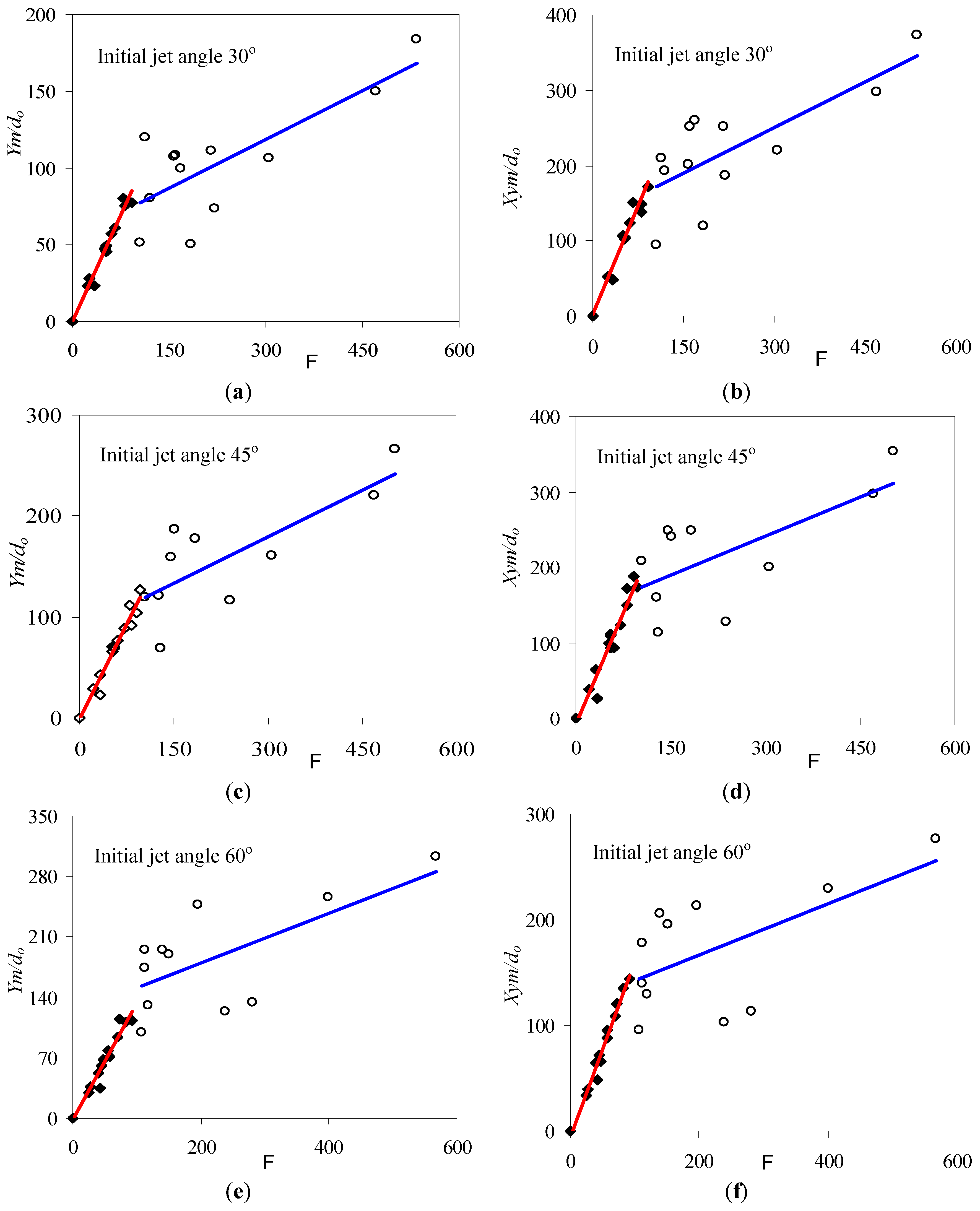
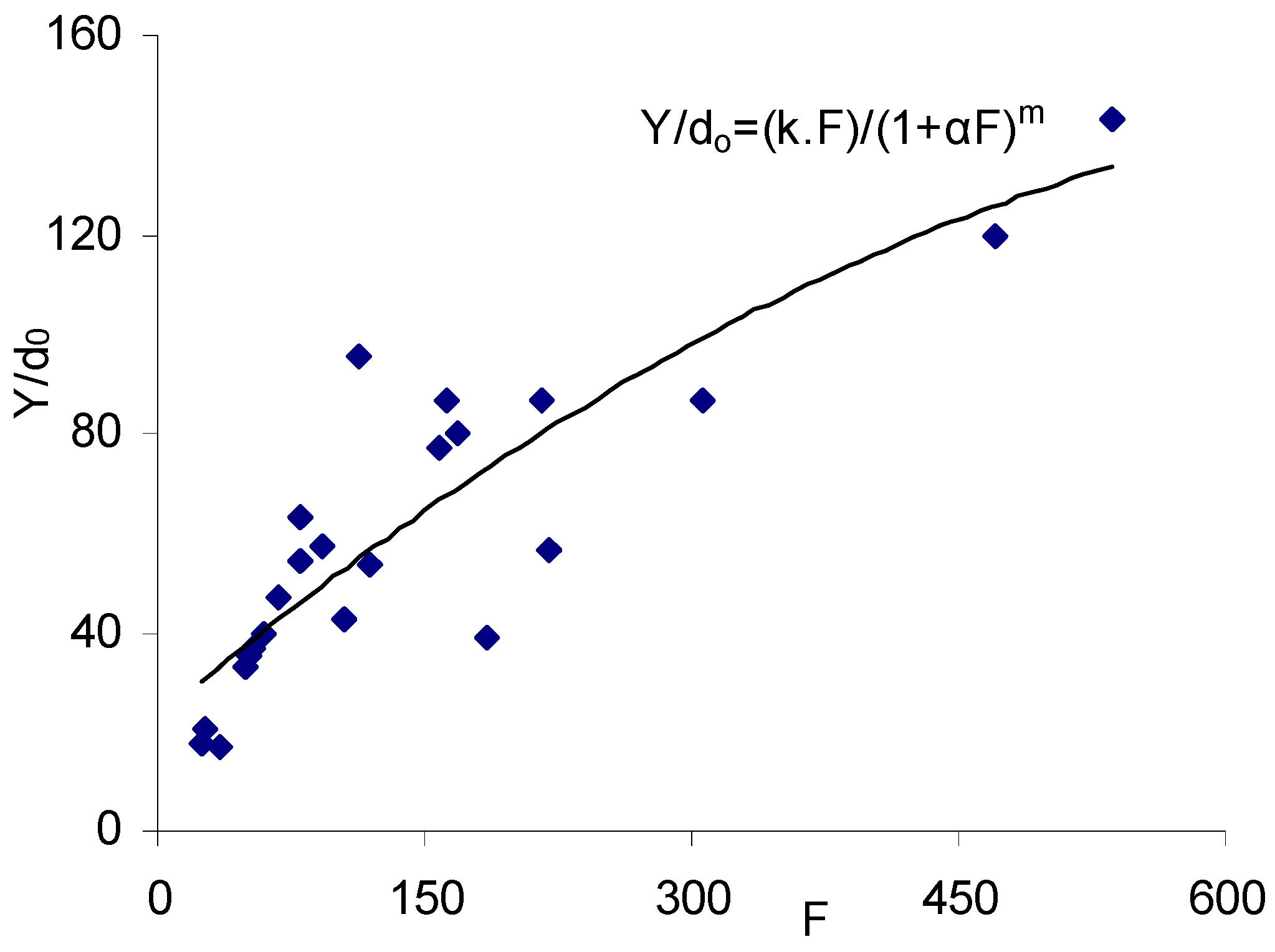
4.3. Densimetric Froude Number Dependence

The dimensional analysis carried out in Section 2.1 showed that the geometric quantities characterizing the jet trajectory should be a function of the densimetric Froude number (F). Thus, Y, X_y, Y_m, and X_ym were normalized with the exit jet diameter (d_o) and plotted versus F separately for the three initial jet angles in order to investigate possible relationships; and to compare with the theoretical analysis and the results of the previous investigation. For all jet quantities studied, there seemed to be a change in behavior at approximately F = 100; below this value the data points closely followed a linear trend, displaying little scatter around the least-square fitted line. For F > 100, the data points exhibited much more scatter.

However, if a straight line was still fitted through the data, the slope of the line was significantly smaller than for F < 100. Figure 7 illustrates Y_m/d_o and X_ym/d_o, as functions of F for the three initial jet angles. Separate least-square best-fitted straight lines were added for the data points above and below F = 100. All other quantities showed the same behavior as Y_m/d_o and X_ym/d_o.

Equation 4 indicates that there is a linear relationship between the normalized quantities that describe the jet trajectory and F. However, this is based on the assumption that l_m >> l_Q, otherwise Equation 3 should be employed. Developing Equation 3 by introducing the definition of the length scales yields,

(7)

where Ψ = function and Y is used as an example of a geometric jet quantity. If F is small Ψ(F) → 1, whereas for large F values Y → ∞. The data indicates a relationship where , with n < 1. Based on the theoretical constraints and the empirical observations, the following equation was proposed to describe Y/d_o as a function of F over the entire range of experimental data,

(8)

where a and m are empirical coefficients obtained from fitting against data. Equation 8 can be approximated with a straight line in accordance with Equation 6 for small values on a F.

Figure 8 shows an example of least-square fitting of Equation 8 against the data for the maximum jet centerline level (Y) and an initial jet angle of 30°, where the optimum values of k, a, and m were determined (1.35, 0.008, and 0.8, respectively). Overall the trend of the data points is well described, but the significant scatter for F > 100 is still present, which discredits the agreement. The other initial angles for Y and the other jet quantities could be fitted about equally well.

Figure 7. Non-dimensional jet quantities Y_m/d_o and X_ym/d_o as a function of F for different initial jet angles (a-f) together with linear regression lines fitted for F-values smaller and larger than 100.

Figure 7. Non-dimensional jet quantities Y_m/d_o and X_ym/d_o as a function of F for different initial jet angles (a-f) together with linear regression lines fitted for F-values smaller and larger than 100.

Figure 8. Normalized maximum jet centerline level as a function of the densimetric Froude number for an initial jet angle of 30°.

Figure 8. Normalized maximum jet centerline level as a function of the densimetric Froude number for an initial jet angle of 30°.

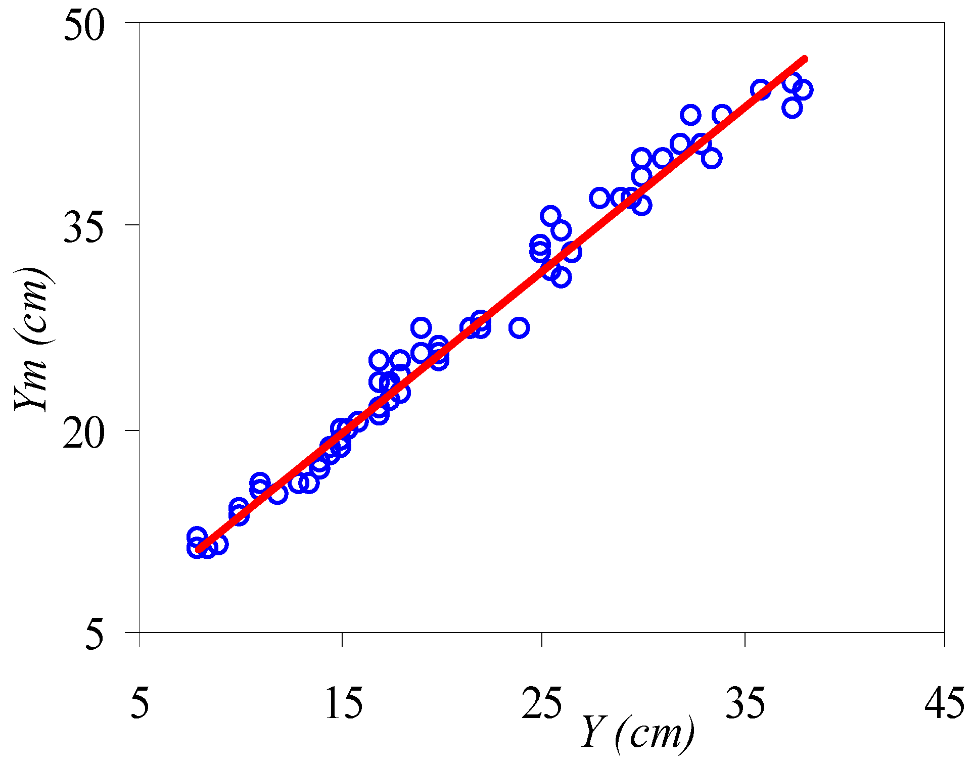
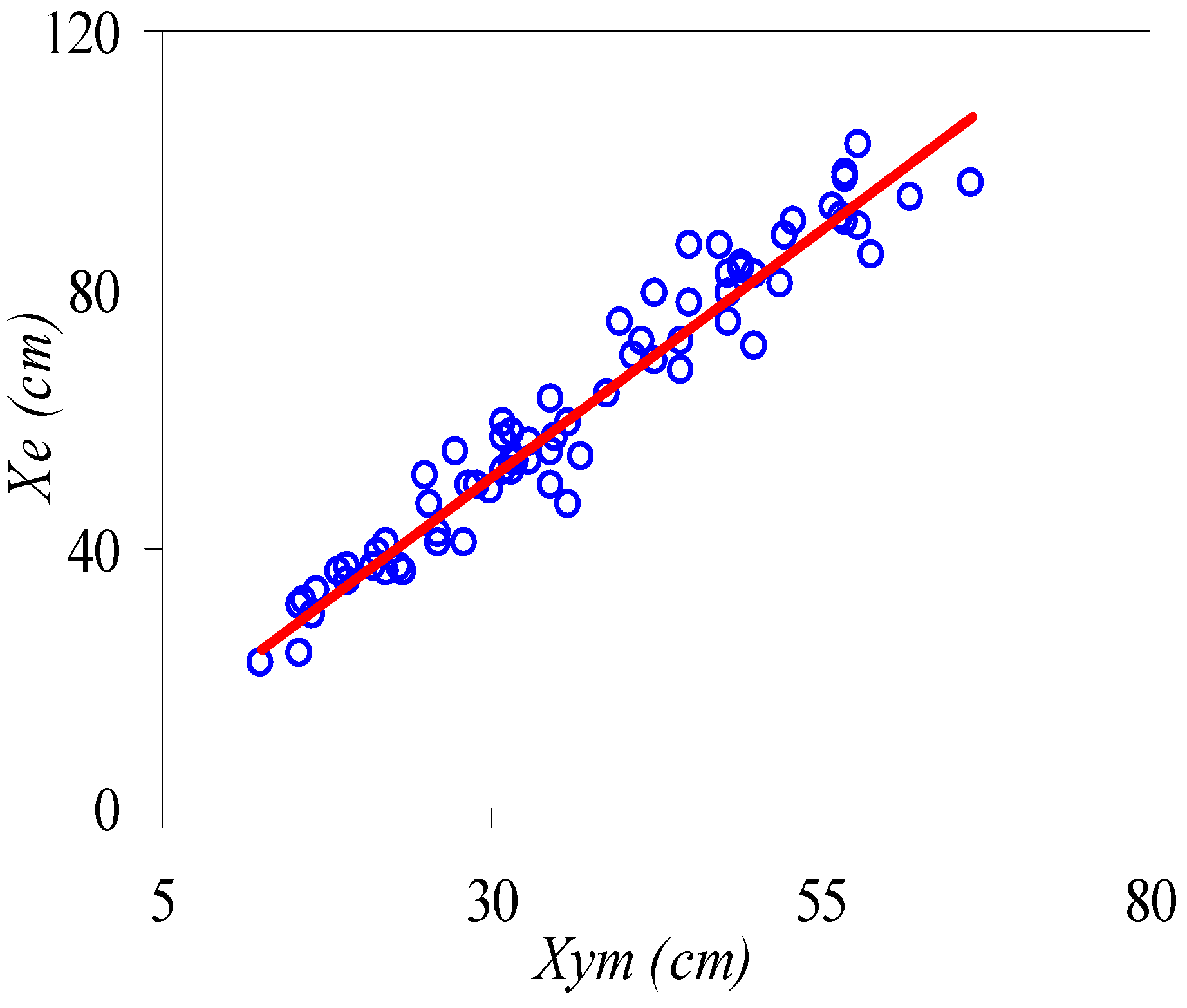
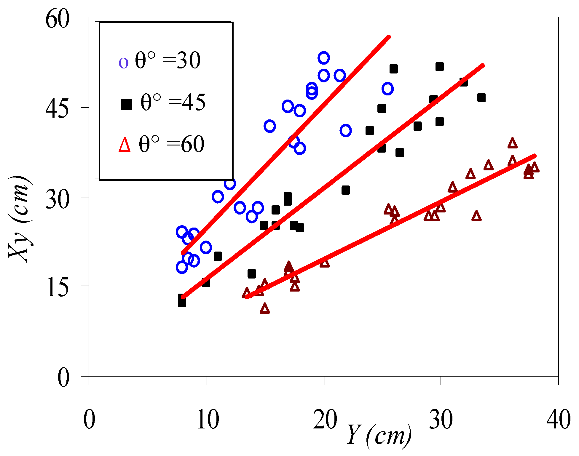
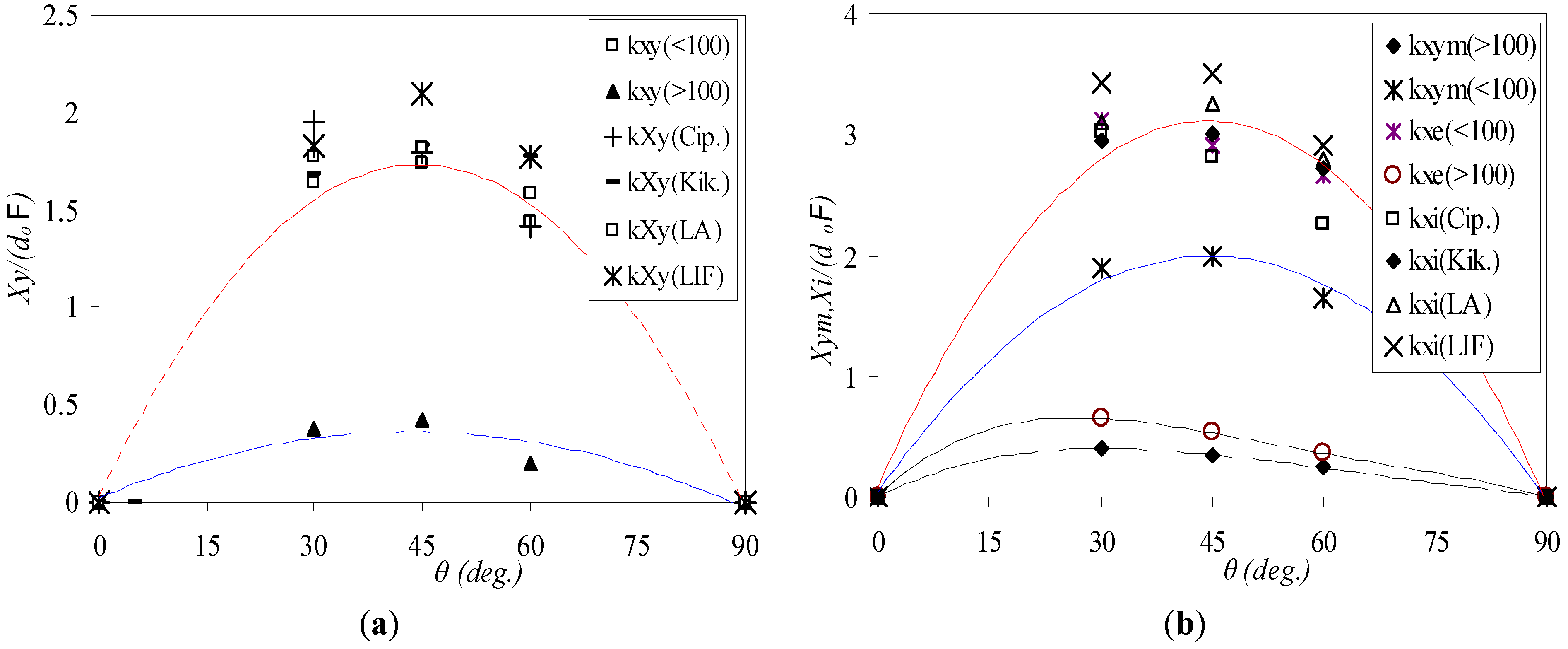
4.4. Relationships for Jet Quantities

Over the range of studied initial jet angles, the variation in the coefficient values with θ is limited, but there is a tendency for these values to decrease with θ (from 30° to 60°). In general, the coefficients obtained in the present study are somewhat lower than those recorded in previous studies. Table 2 summarizes the coefficient values found for the vertical and horizontal distances investigated for F above and below 100 (corresponding values from previous studies are also shown in Table 2). The subscript of k in the table corresponds to the specific geometric quantities previously discussed, with the exception of X_i, which is the distance to the jet impact point (where the jet centerline encounters the level of the jet nozzle; see Figure 1).

Table 2. Coefficient values describing the linear dependence of normalized geometric jet quantities on the densimetric Froude number compared to previous investigations and predictions.

Study angle ( θ0)	ky			kym			kxe
	30°	45°	60°	30°	45°	60°	30°	45°	60°
Zeitoun et al. [28]	-	-	-	1.04	1.56	2.13	-	-	-
Lindberg [14]	-	-	-	1.29	1.58	2.14	-	-	-
Bloomfield & Kerr [29]	-	-	-	0.89	1.24	1.63	-	-	-
Cipollina et al. [15]	0.79	1.17	1.77	1.08	1.61	2.32	3.03	2.82	2.25
Kikkert LA (1) [30]	0.61	1.1	1.6	1.07	1.71	2.28	3.18	3.32	2.79
Kikkert LIF (2) [30]	-	1.21	1.76	1.21	1.78	2.45	-	-	-
Kikkert et al. (3) [16]	0.63	1.14	1.70	1.07	1.66	2.27	2.96	3.05	2.72
Papakonstantis et al. [18]	-	-	-	-	1.45	1.99	-	-	-
Papakonstantis [31]	-	1.17	1.68	-	1.58	2.14	-	3.16	2.75
Christodoulou & Papak. [20]	0.62	1.27	1.89	1.12	1.59	2.14	3.18	3.16	2.75
Papakonstantis et al. [31]	-	-	-	-	1.58	2.14	-	3.78	3.57
This study: F < 100	0.69	1.0	1.4	0.92	1.3	1.7	3.12	2.90	2.66
F > 100	0.17	0.26	0.24	0.21	0.31	0.29	0.65	0.53	0.36

Table 2. Coefficient values describing the linear dependence of normalized geometric jet quantities on the densimetric Froude number compared to previous investigations and predictions.

Study angle ( θ0)	ky			kym			kxe
	30°	45°	60°	30°	45°	60°	30°	45°	60°
Zeitoun et al. [28]	-	-	-	1.04	1.56	2.13	-	-	-
Lindberg [14]	-	-	-	1.29	1.58	2.14	-	-	-
Bloomfield & Kerr [29]	-	-	-	0.89	1.24	1.63	-	-	-
Cipollina et al. [15]	0.79	1.17	1.77	1.08	1.61	2.32	3.03	2.82	2.25
Kikkert LA (1) [30]	0.61	1.1	1.6	1.07	1.71	2.28	3.18	3.32	2.79
Kikkert LIF (2) [30]	-	1.21	1.76	1.21	1.78	2.45	-	-	-
Kikkert et al. (3) [16]	0.63	1.14	1.70	1.07	1.66	2.27	2.96	3.05	2.72
Papakonstantis et al. [18]	-	-	-	-	1.45	1.99	-	-	-
Papakonstantis [31]	-	1.17	1.68	-	1.58	2.14	-	3.16	2.75
Christodoulou & Papak. [20]	0.62	1.27	1.89	1.12	1.59	2.14	3.18	3.16	2.75
Papakonstantis et al. [31]	-	-	-	-	1.58	2.14	-	3.78	3.57
This study: F < 100	0.69	1.0	1.4	0.92	1.3	1.7	3.12	2.90	2.66
F > 100	0.17	0.26	0.24	0.21	0.31	0.29	0.65	0.53	0.36

The slopes of the least-square fitted straight lines discussed in the previous section were determined for the different jet quantities, separating data points below and above F = 100. The obtained slope coefficients for the normalized maximum jet levels Y (ky) and Y_m (ky_m) as a function of F are shown (see Figure 9). The coefficient values seem to increase with the initial jet angle in a linear manner, although the number of points was limited. Figure 9 also includes corresponding coefficient values found in earlier studies, which have reported the same trend. These values originate from four different sources [15,16] with values predicted from their analytical model, and measured by the light attenuation system (LA), and laser-induced fluorescence system (LIF).

The values for ky and ky_m are listed in (Table 2) with respect to the three initial jet angles (30°, 45°, and 60°). For example, the values obtained for ky_m at 30° were 0.92 (F < 100) and 0.21 (F > 100) compared to the value reported by Cipollina et al. [15] of 1.08, which was obtained for F < 100. Thus, for this case the agreement is good; however, for the larger angles the deviation between the coefficient values (ky and ky_m) obtained in this study and in previous studies is larger than for the smaller angles. As mentioned before, besides differences in experimental setups and procedures, a reason for the discrepancies between experiments may be due to the marked differences in some of the input parameters not described by the non-dimensional quantities employed. For example, Cipollina et al. [15] used densities in the jet which were much larger than in the present experiment, and also much larger than that expected in brine jets. The slope coefficients for the horizontal distance to the maximum jet centerline level (kx_y), to the maximum jet edge level (kx_ym), and to the edge point (kx_e) were also determined with regard to the initial jet angle and whether F was above or below 100 (see Figure 10).

Figure 9. Slope coefficient for (a) maximum jet centerline level (ky = Y/(d₀F)); and (b) maximum jet edge level (ky_m = Y_m/(d₀F)) as a function of initial jet angle for densimetric Froude number below and above 100, together with results from previous studies.

Figure 9. Slope coefficient for (a) maximum jet centerline level (ky = Y/(d₀F)); and (b) maximum jet edge level (ky_m = Y_m/(d₀F)) as a function of initial jet angle for densimetric Froude number below and above 100, together with results from previous studies.

Figure 10. Slope coefficient for horizontal distance to (a) maximum jet centerline level(kx_y = X_y/(d₀F)); and (b) maximum jet edge level(kx_ym = Xym/(d₀F)) as a function of jet angle for densimetric Froude number below and above 100, together with results from previous studies.

Figure 10. Slope coefficient for horizontal distance to (a) maximum jet centerline level(kx_y = X_y/(d₀F)); and (b) maximum jet edge level(kx_ym = Xym/(d₀F)) as a function of jet angle for densimetric Froude number below and above 100, together with results from previous studies.

Furthermore, previously obtained corresponding values reported in [15,16] were included for comparison. The dependence of the coefficients for the horizontal distances on the initial jet angle are quite different from the vertical distances, and two extra points may be added on theoretical grounds, namely at θ = 0° and 90° for which the distance should be zero [15]. A polynomial was fitted through the data of five points, but the shape of the curve outside the measurement points has little support. It appears that there are small differences between this study and previous study results; this may indicate that buoyancy becomes important after some distance for the discharge point. It is also possibly from the boundary interactions of the tank sides and its limited depth.

5. Conclusions

A laboratory experiment was conducted to investigate the behavior of negatively buoyant jets discharged at an angle to the horizontal into a quiescent body of water. Several of the geometric jet quantities showed strong correlation and regression relationships could be developed where one quantity could be predicted from another. If maximum levels were correlated with the corresponding horizontal distances, the angle must be taken into account when developing predictive relationships in real life projects.

Analysis of the collected data showed that this was the case for a Froude number smaller than 100, whereas for larger values the scatter in the data increased significantly. The slope of the best-fit straight line through the data points was a function of the initial jet angle, where the slope increased with angle for the maximum levels studied, but had a more complex behavior for horizontal distances. It is believed that the empirical relationships developed in this study have a potential for use in practical design where the trajectory of brine jets needs to be estimated, if the Froude number is less than 100. Equations were proposed to relate levels or horizontal distances to each other.

Inclined negatively buoyant jet is an efficient method to improve the dilution rate of brine discharged from a desalination plant into the receiver. In this study, it was observed that the initial jet angle (θ) is important as it shows a better dilution rate improvement when it is 60° than 30° or 45°. This result can easily be applied to existing and future desalination plant discharges. Thus, the effects of brine discharge should be considered in all future study and design of desalination plants.

References

1. Turner, J.S. Jets and plumes with negative or reversing buoyancy. J. Fluid Mech. 1966, 26, 779–792. [Google Scholar] [CrossRef]
2. Abraham, G. Jets with negative buoyancy in homogeneous fluids. J. Hydraul. Res. 1967, 5, 236–248. [Google Scholar]
3. Tong, S.S.; Stolzenbach, K.D. Submerged Discharges of Dense Effluent; Report No. 243; Massachusetts Institute of Technology: Cambridge, MA, USA, 1979. [Google Scholar]
4. James, W.P.; Vergara, I.; Kim, K. Dilution of a dense vertical jet. J. Environ. Eng. 1983, 109, 1273–1283. [Google Scholar] [CrossRef]
5. McLellan, T.N.; Randall, R. Measurement of brine jet height and dilution. J. Waterw. Port Coast Ocean Eng. 1986, 112, 200–216. [Google Scholar] [CrossRef]
6. Baines, W.D.; Turner, J.S.; Campbell, I.H. Turbulent fountains in an open chamber. J. Fluid Mech. 1990, 212, 557–592. [Google Scholar] [CrossRef]
7. Roberts, P.J.W.; Toms, G. Inclined dense jets inflowing current. J. Hydraul. Eng. 1987, 113, 323–341. [Google Scholar] [CrossRef]
8. Roberts, P.J.W.; Toms, G. Ocean outfall system for dense and buoyant effluents. J. Environ. Eng. 1988, 114, 1175–1191. [Google Scholar] [CrossRef]
9. Roberts, P.J.W.; Ferrier, A.; Daviero, G. Mixing in inclined dense jets. J. Hydraul. Eng. 1997, 123, 693–699. [Google Scholar] [CrossRef]
10. Zhang, H.; Baddour, R.E. Maximum penetration of vertical round dense jets at small and large Froude numbers. J. Hydraul. Eng. 1998, 124, 550–553. [Google Scholar] [CrossRef]
11. Zeitoun, M.A.; Reid, R.O.; McHilhenny, W.F.; Mitchell, T.M. Model Studies of Outfall Systems for Desalination Plants; Research and Development Progress Report No. 804; Office of Saline Water,U.S. Department of the Interior: Washington, DC, USA, 1972. [Google Scholar]
12. Pincince, A.B.; List, E.J. Disposal of brine into an estuary. J. Water Polllut. Control Fed. 1973, 45, 2335–2344. [Google Scholar]
13. Demetriou, J.D. Turbulent Diffusion of Vertical Water Jets with Negative Buoyancy (In Greek). Ph.D. Dissertation, National Technical University of Athens, Athens, Greece, 1978. [Google Scholar]
14. Lindberg, W.R. Experiments on negatively buoyant jets, with and without cross-flow. In Recent Research Advances in the Fluid Mechanics of Turbulent Jets and Plumes; Davies, P.A., Valente Neves, M.J., Eds.; Springer: Berlin, Germany, 1994; Volume 255, pp. 131–145. [Google Scholar]
15. Cipollina, A.; Brucato, A.; Grisafi, F.; Nicosia, S. Bench scale investigation of inclined dense jets. J. Hydraul. Eng. 2005, 131, 1017–1022. [Google Scholar] [CrossRef]
16. Kikkert, G.A.; Davidson, M.J.; Nokes, R.I. Inclined negatively buoyant discharges. J. Hydraul. Eng. 2007, 133, 545–554. [Google Scholar] [CrossRef]
17. Jirka, G.H. Integral model for turbulent buoyant jets in unbounded stratified flows. Part 2: Plane jet dynamics resulting from multiport diffuser jets. Environ. Fluid Mech. 2006, 6, 43–100. [Google Scholar] [CrossRef]
18. Papakonstantis, I.; Kampourelli, M.; Christodoulou, G. Height of rise of inclined and vertical negatively buoyant jets. In Proceedings of 32nd IAHR Congress, Venice, Italy, 1–6 July 2007 [CD-ROM]; IAHR (The International Association for Hydro-Environment Engineering and Research): Madrid, Spain, 2004. [Google Scholar]
19. Jirka, G.H. Improved discharge configuration for brine effluents from desalination plants. J. Hydraulic Eng. 2008, 134, 116–120. [Google Scholar] [CrossRef]
20. Christodoulou, G.C.; Papakonstantis, I.G. Simplified estimates of trajectory of inclined negatively buoyant jets. In Environmental Hydraulics; Taylor & Francis: London, UK, 2010; pp. 165–170. [Google Scholar]
21. Ferrari, S.; Querzoli, G. Mixing and re-entrainment in a negatively buoyant jet. J. Hydraul. Res. 2010, 48, 632–640. [Google Scholar] [CrossRef]
22. Papakonstantis, I.G.; Christodoulou, G.C.; Papanicolaou, P.N. Inclined negatively buoyant jets 1: Geometrical characteristics. J. Hydraul. Res. 2011, 49, 3–12. [Google Scholar] [CrossRef]
23. Sanchez, M.D. Near-Field Evolution and Mixing of a Negatively Buoyant Jet Consisting of Brine from a Desalination Plant. Master’s Thesis, Water Resources Engineering, Department of Building and Environmental Technology, Lund University, Lund, Sweden, 2009. [Google Scholar]
24. Fischer, H.B.; List, E.J.; Koh, R.C.Y.; Imberger, J.; Brooks, N.H. Mixing in Inland and Coastal Waters; Academic Press: New York, NY, USA, 1979. [Google Scholar]
25. Wright, S.J. Buoyant jets in density-stratified crossflow. J. Hydraul. Eng. 1984, 110, 643–656. [Google Scholar] [CrossRef]
26. Doneker, R.L.; Jirka, G.H. Cormix User Manual 6.0E: A Hydrodynamic Mixing Zone Model and Decision Support System for Pollutant Discharges into Surface Waters; U.S. Environmental Protection Agency: Washington, DC, USA, 2007. [Google Scholar]
27. Fan, L.-N.; Brooks, N.H. Dilution of Waste Gas Discharge from Campus Buildings; Technical Memo 68-1; California Institute of Technology: Pasadena, CA, USA, 1968. [Google Scholar]
28. Zeitoun, M.A.; McHilhenny, W.F.; Reid, R.O. Conceptual Designs of Outfall Systems for Desalination Plants; Research and Development Progress Report No. 550; Office of Saline Water, U.S. Department of the Interior: Washington, DC, USA, 1970. [Google Scholar]
29. Bloomfield, L.J.; Kerr, R.C. A theoretical model of a turbulent fountain. J. Fluid Mech. 2000, 424, 197–216. [Google Scholar] [CrossRef]
30. Kikkert, G.A. Buoyant Jets with Two and Three Dimensional Trajectories. Ph.D. Dissertation, University of Canterbury, Christchurch, New Zealand, 2006. [Google Scholar]
31. Papakonstantis, I.G. Turbulent Round Negatively Buoyant Jets at an Angle in a Calm Homogeneous Ambient (in Greek). Ph.D. Dissertation, School of Civil Engineering, National Technical University of Athens, Athens, Greece, 2009. [Google Scholar]