Article

Remote Sensing Analysis of Lake Dynamics in Semi-Arid Regions: Implication for Water Resource Management. Lake Manyara, East African Rift, Northern Tanzania

by
Dorothea Deus
1,2,* and
Richard Gloaguen
1,3
1
Remote Sensing Group, Institute of Geology, Faculty of Geosciences, Geoengineering and Mining, Freiberg University of Mining and Technology (TUBAF), Bernhard-von-Cotta Str. 2, Freiberg D-09596, Germany
2
Department of Geomatics, School of Geospatial Sciences and Technology (SGST), Ardhi University, P.O. Box 35176, Dar es Salaam, Tanzania
3
Remote Sensing Group, Helmholtz Institute Freiberg of Resource Technology, Halsbrueckerstr. 34, Freiberg D-09599, Germany
*
Author to whom correspondence should be addressed.
Water 2013, 5(2), 698-727; https://doi.org/10.3390/w5020698
Submission received: 8 April 2013 / Revised: 18 May 2013 / Accepted: 27 May 2013 / Published: 6 June 2013

Abstract

:
We show here that a remote sensing (RS) approach is a cost-efficient and accurate method to study water resource dynamics in semi-arid areas. We use a MODIS surface reflectance dataset and a Modified Normalized Difference Water Index (MNDWI) to map the variability of Lake Manyara’s water surface area using a histogram segmentation technique. The results indicate that Lake Manyara’s water surface coverage has been decreasing from 520.25 km2 to 30.5 km2 in 2000 and 2011 respectively. We observe that the lake water surface and the lake water balance displayed a similar pattern from 2006 to 2009, probably initiated by heavy rainfall and low temperature in 2006. Lake water surface area appears to have an inverse relationship with MODIS evapotranspiration (ET) and MODIS land surface temperature (LST). We imply that recent fluctuations of Lake Manyara’s surface water area are a direct consequence of global and regional climate fluctuations. We therefore conclude that, by means of RS it is possible to provide timely and up-to-date water resource information to managers and hence enable optimized and operational decisions for sustainable management and conservation. We suggest that the method employed in this research should be applied to monitor water resource dynamics provided that remotely sensed datasets are available.

Graphical Abstract

1. Background

Water resources are crucial to human health and the natural environment [1]. Water resources include surface water, groundwater, inland water, rivers, lakes, transitional waters, coastal waters and aquifers [2]. Over time, water resources have been degraded and exhausted. In this study we look at lake water resources. Lakes are key tools for the management of water resources [3]. They are essential component of the hydrological cycle [4]. Monitoring lake dynamics is necessary to allow sustainable management of water resources. In addition, lake surface areas, especially closed lakes, are known for their sensitivity to natural changes and thus may serve as important proxies for regional environmental and global climate fluctuations [4,5]. Changes in the areal extent of lake surface water may occur due to various factors including progressive infilling of the lake basin by sediments, climate change, tectonic activity causing uplift and subsidence, or the development of drainage faults [6,7]. Goerner et al. [7] pointed out that surface pressure, wind-driven events such as seiches and tides, alternating water temperature or composition, and modifications of water circulation processes can all influence lacustrine water depth.
Detecting and characterizing changes over time is the natural first step toward identifying the driver of the change and understanding the change mechanism [8]. Changes in lake level or relative water depth are both functions of lake surface and volume. It is important to understand lake water surface and storage changes to be able to assess the influence of climate variation or human activities on water resources [9]. Although a number of studies have been conducted on East African rift lakes, Lake Manyara’s surface fluctuations have not yet been thoroughly studied. It was heretofore unknown if lake fluctuations were seasonal or inter-annual or related to climate. Precise and up to date information on the status and trends of lake surface dynamics is needed to enable the development of effective strategies for sustainable management of lakes and the assessment of environment change. Water managers cannot manage what they do not know. Therefore, a necessity for accurate spatial and temporal information on water resources continuously is evident for enhanced management.
Accurate water surface quantification and mapping demands correct delineation and estimation of the spatial and temporal dissemination of the water resource. Traditional in situ data measurement methods that produce representative spatial and temporal information on water resources are costly. Remote sensing is the most economical technique for the monitoring of lake dynamics. Remote sensing has been used in various studies to monitor and analyze lacustrine water dynamics [4,7,10]. We use remote sensing to quantify the variation in Lake Manyara’s surface water areal extent from 2000 to 2011. Water extraction from remote sensing images can be divided into single band and multi-band techniques [11]. Normally, for the single band method a threshold for the band is applied to differentiate water information from land information. This technique has the disadvantage that water surface may be over or under estimated, and/or may be mixed with shadow noise due to the intuitive selection of threshold. The multiband technique has the advantage of using distinctive reflective capabilities of water surfaces in various bands. A number of multiband water indices have been developed and employed recently in the field. These make use of either the water indices threshold segmentation approach [4,11,12,13,14] or the step-wise iterative transformation mechanism [15].
Over the past two decade, satellite remote sensing has shown promising result in estimation of water resource storage in large reservoirs and lakes [3]. However, the purpose of this study is to show the potential of remote sensing techniques in assessment of water resources surface dynamics (the case of smaller lakes and reservoirs). To support sustainable management and conservation of the water resources in semi-arid environment and areas in needy like Africa where a large number of people depend on smaller lakes or reservoirs for water resources. The objective of this work is two-fold; (1) assess the efficacy of remote sensing-based lake monitoring and (2) infer the probable causes for lake change and consequent vegetation adaptation in order to contribute toward sustainable environment management. We map, analyze and quantify the historical lake surface variation, identifying annual variations. We evaluate the lake water cycle from 2002 to 2009 as compared to the lake water level/surface variation. We show the potential of the water index approach in water resource surface delineation and mapping. We also assess the capabilities of different remote sensing indices in detecting and differentiating water resources from non-water features, suggesting the optimal water index for water resource assessment and monitoring.

2. Study Area and Data
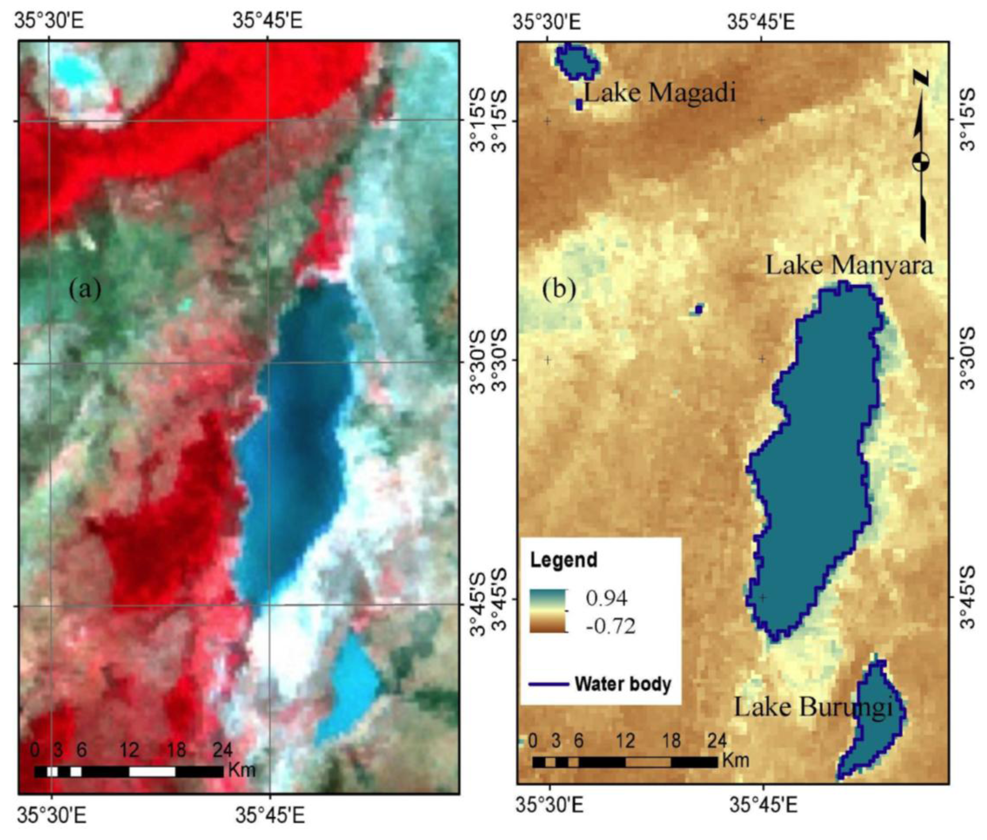
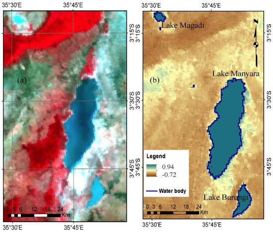
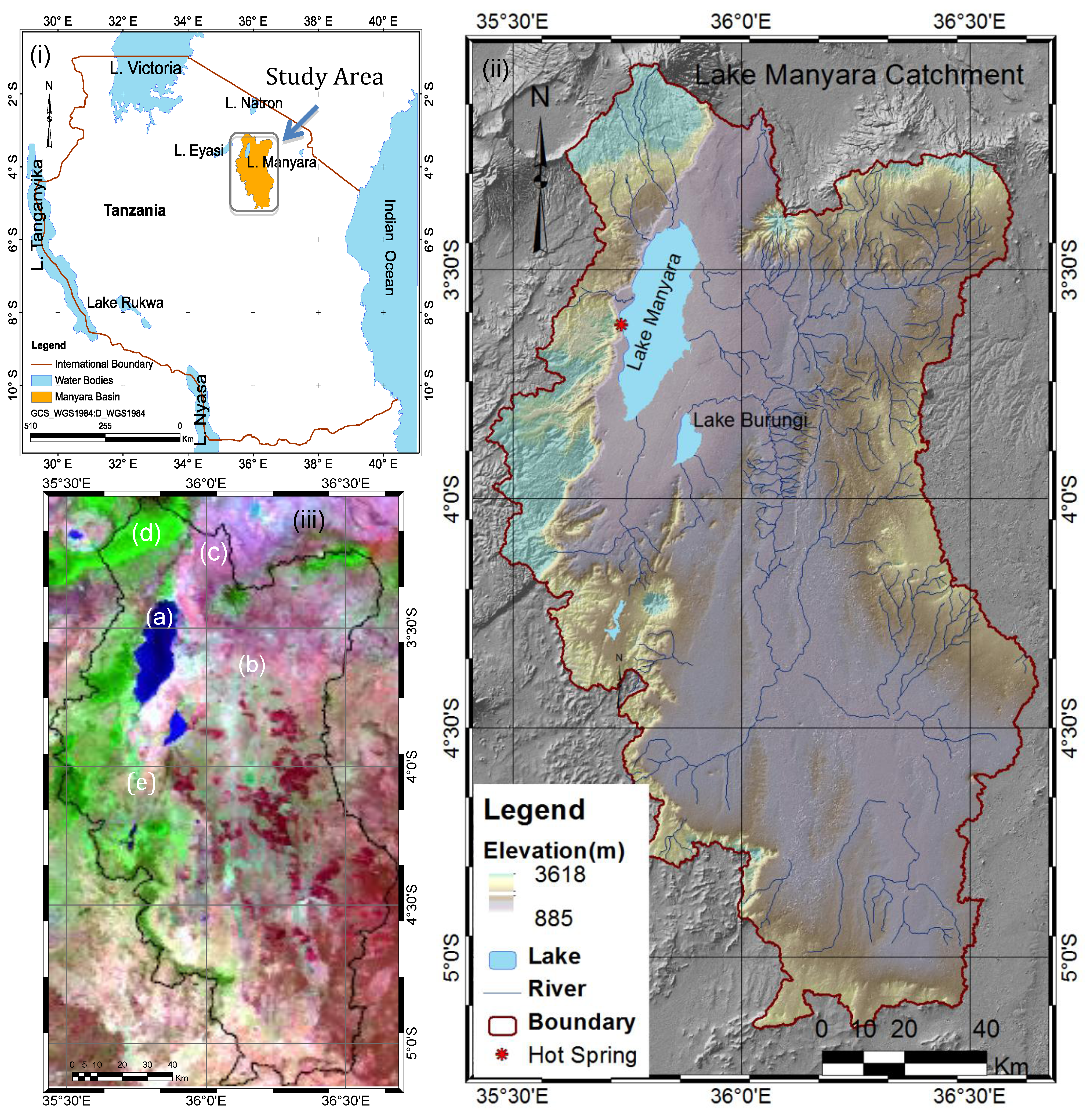
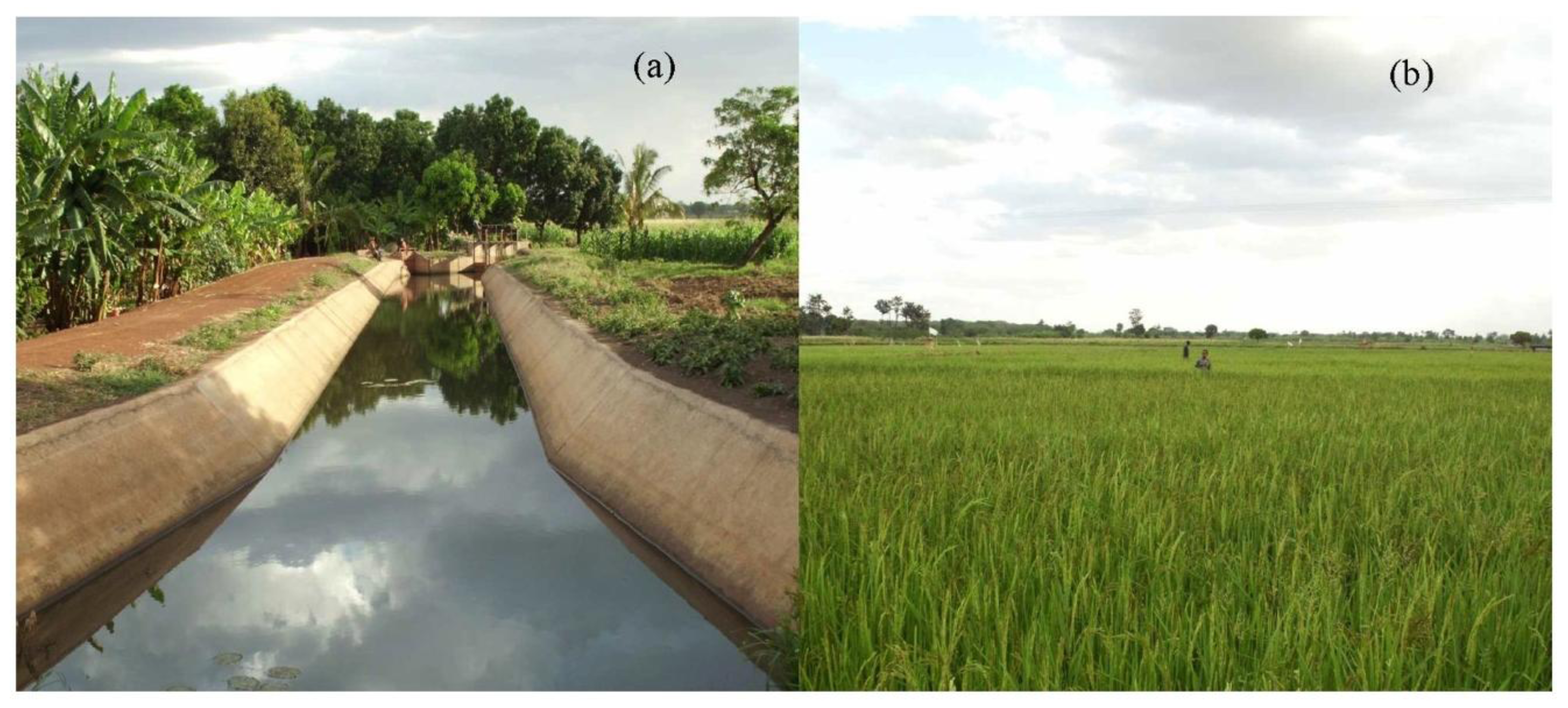
2.1. Study Area

Lake Manyara is the southernmost lake within the eastern arm of the East African rift system [16,17]. The lake is shallow and saline and located 126 km west of Arusha in northern Tanzania (3°25′–3°48′ S, 35°44′–35°53′ E, 960 m above sea level (a.s.l) (Figure 1). The maximum lake area is 520.5 km2, based on a Landsat Multispectral Scanner (MSS) satellite image acquired on 22 September 1973. The lake has on several occasions dried-up completely. In 2010, the average water depth was as low as 1.18 m. The Lake Manyara catchment area covers about 18,740 km2 and lies between 885 m and 3618 m a.s.l. It is a closed basin with no outlet. A deep escarpment flanks the western side of the lake and in the east an undulating plain with isolated volcanic cones gives way to a peneplain. Several springs and streams, both perennial and seasonal, drain into the lake [17].
The climate of the Lake Manyara catchment is principally influenced by a seasonal shift of the Inter-tropical Convergence Zone (ITCZ) that has a strong effect in East Africa [18,19]. Highly seasonal and annually variable rainfalls total approximately 600 mm/yr (Figure 2). The rainy season lasts from November to May with a short and a long rainy season. The dry season ranges from June to October and extends when the short rainy season fails [20,21]. Annual mean air temperature at the lake ranges between 15 °C and 25 °C (Figure 2).
Figure 1. Lake Manyara catchment–Study area: (i) Map of Tanzania displaying the location of Lake Manyara catchment in northern Tanzania; (ii) Lake Manyara and its catchment; (iii) Some land cover classes with regarding to Moderate resolution Imaging Spectro-radiometer (MODIS) surface reflectance image (False color composite band 742 acquired on 16 August 2010; (a) Water; (b) Shrubs/grasslands; (c) Sand/Bare soils; (d) Dense forest; (e) Moderate forest.
Water 05 00698 g001
Figure 2. Annual rainfall pattern and temperature variation within Lake Manyara catchment during study period.
Water 05 00698 g002

2.2. Data

2.2.1. Satellite Data

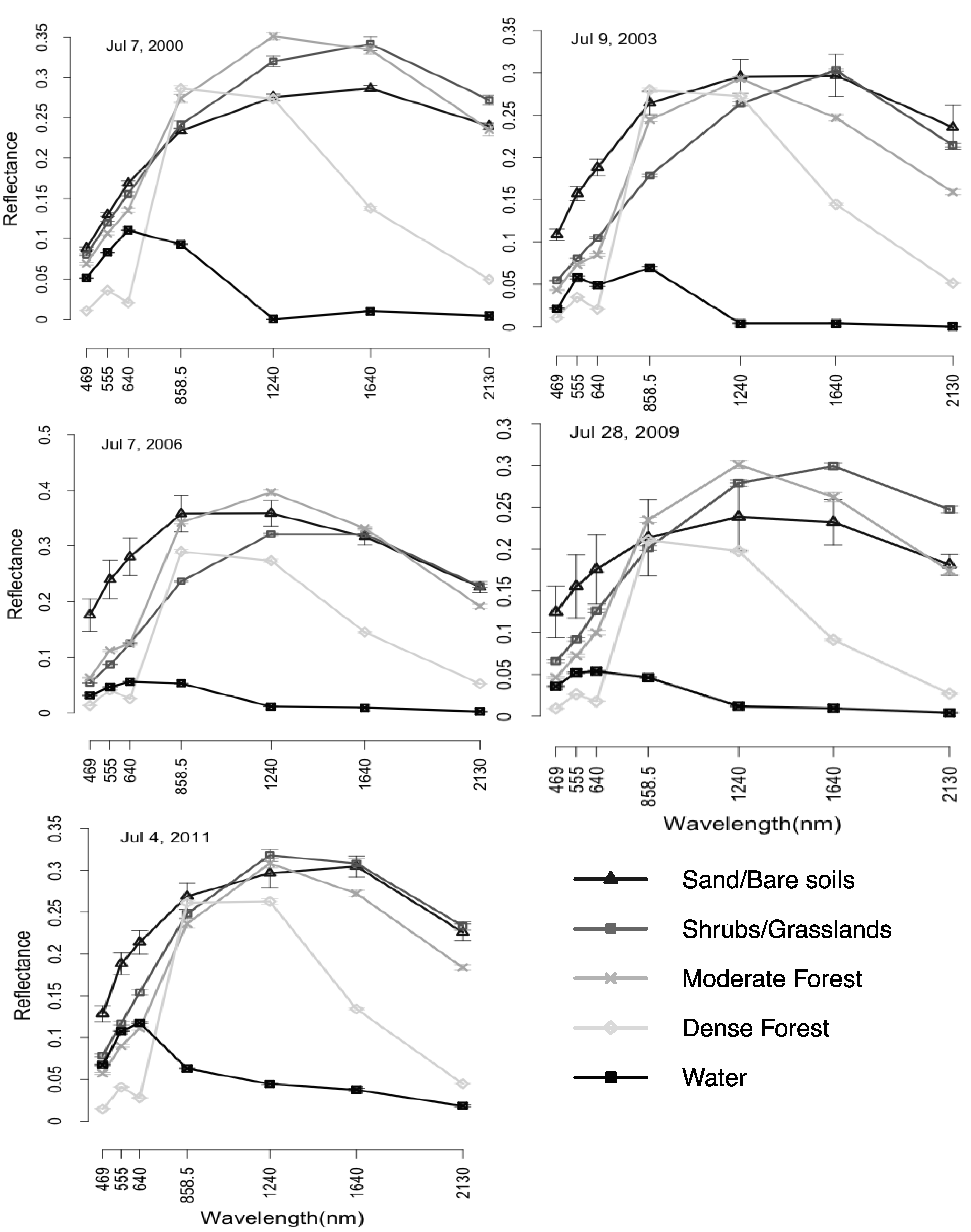
(a) MODIS Land Surface Reflectance

We use multi-temporal satellite images to study Lake Manyara surface dynamics. A Landsat MSS scene acquired on 22 September 1973 was used to map the lake coastline. We use atmospherically corrected Moderate resolution Imaging Spectro-radiometer (MODIS) Terra surface reflectance product (MOD09GA, Version 4 [22] to map and monitor Lake Manyara water surface spatial and temporal variations from 2000 to 2011. We selected data acquired in the dry season (June–October) to avoid obstruction from clouds and we apply a scale factor of 0.0001 to every scene. Surface reflectance typically ranges from 0 to 1. MOD09GA surface reflectance product values are scaled by 10,000 and then cast to 16-bit integers, therefore surface reflectance values in MOD09GA image files vary between 0 and 10,000 [22]. So we use the scale factor of 0.0001 to convert the values to float such that they range from 0 to 1. All selected data were cloud free or nearly cloud free (less than 10%). Despite its medium spatial resolution (500 m) the MODIS surface reflectance dataset is appropriate for monitoring surface water dynamics and differentiating between land cover types due to its high spectral resolution and the frequency of observations. MOD09GA is a seven-band surface reflectance daily product computed from the MODIS Level 1B land surface data bands 1 (620–670 nm), 2 (841–876 nm), 3 (459–479 nm), 4 (545–565 nm), 5 (1230–1250 nm), 6 (1628–1652 nm), and 7 (2105–2155 nm) [22].
Apart from the MOD09GA surface reflectance product, we use MCD43A4 [22] to assess the lake surface variability during the wet and dry seasons on a monthly basis. This is a 16-day MODIS Terra and Aqua combined product that provides global adjusted surface reflectance data at nadir using a bi-directional reflectance distribution function (BRDF). Since the data are corrected anisotropically they can serve as important inputs for studies using vegetation indices and for land cover classification [23]. The dataset has a spatial resolution of 500 m.

(b) MODIS Land Surface Temperature

We used MODIS/Terra (Earth Observing System (EOS) AM- 1 platform) daily daytime MOD11C1 V5 land surface temperature (LST) product at a spatial resolution of 0.05° (~5600 m) [24]. MOD11C1 V5 product generation executive code (PGE16) has been refined to account for surface elevation as well as exclusion of temporal averaging and cloud-contaminated LSTs in level-3 LST products, and the modifications of the day/night LST algorithm [24]. The dataset is available from March 2000 to date. MOD11C1 V5 LSTs product has been compared in 47 clear-sky cases with in situ measurement and its accuracy is better than 1K in the range from −10° to 58 °C in about 39 cases [24].

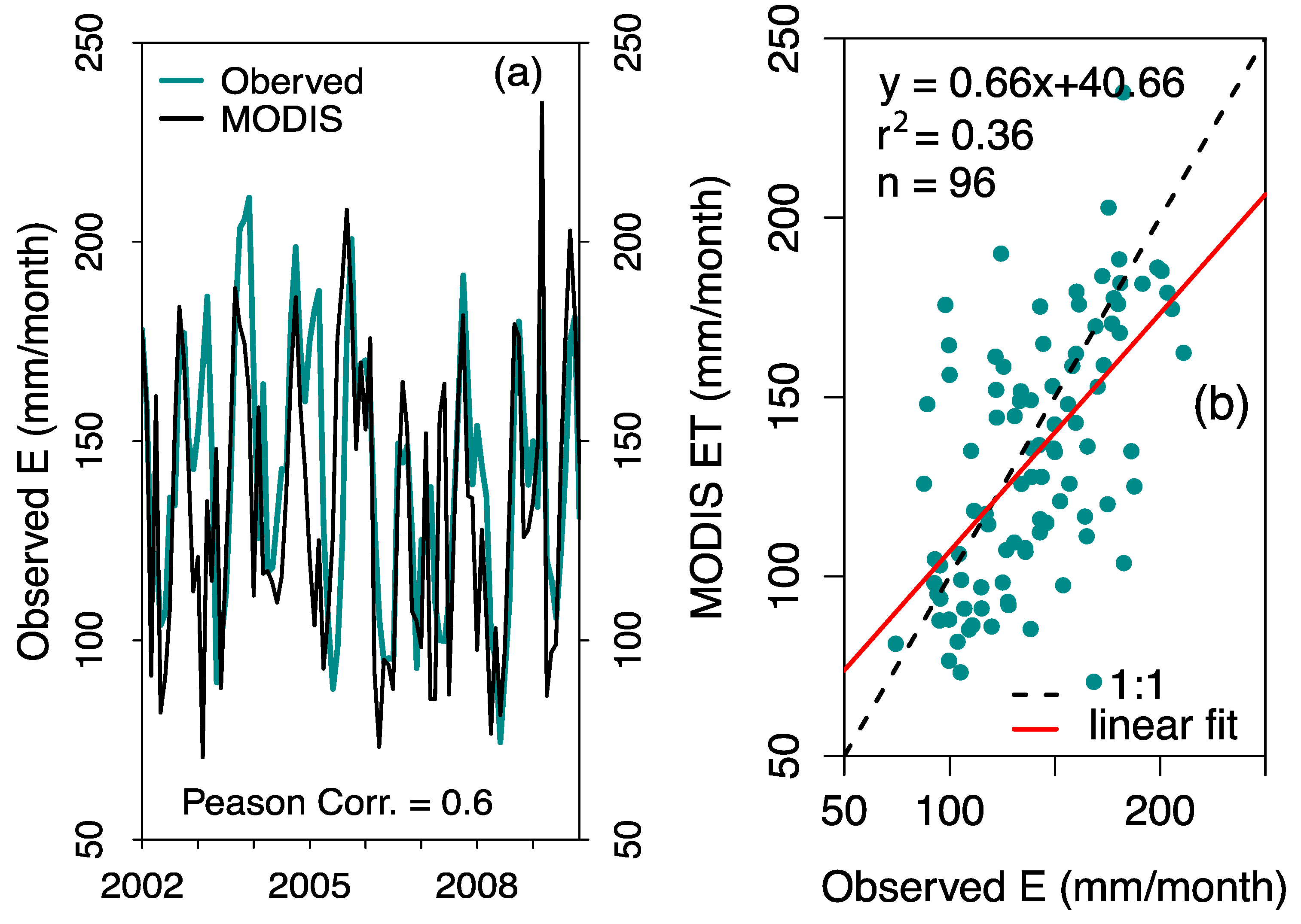
(c) MODIS Evapotranspiration

Evapotranspiration (ET) is an important factor for understanding hydrological processes and climate dynamics [25]. ET depends on soil moisture, vegetation types and on meteorological parameters such as wind speed, air temperature, solar radiation and humidity. We use MODIS global ET (MOD16A2) product with a spatial resolution of 1 km and a temporal resolution of 8 days [26,27]. The dataset is available from 1 January 2000 to 27 December 2009 and can be accessed using the MODIS global land product subset tool provided by Oak Ridge National Laboratory Distributed Active Archive Center (ORNL DAAC) [28]. MODIS provides evapotranspiration data for the regional and global hydrological cycle [26]. Bookhagen and Burbank, [29] demonstrated that MODIS-derived evapotranspiration amounts has the potential to allows accurate prediction of discharge amounts. MOD16 ET products have been validated using flux tower observations from 17 sites in Asia, the stations have different geological and meteorological backgrounds [30]. The agreement between MODIS-based ET and ET observed at the flux towers ranged from a correlation of 0.50 to 0.76 with a RMSE of 1.99 to 8.96 mm in forest land [30]. Tang et al. [31] validated MODIS ET in semiarid environments, and found that they reasonably fit with in situ based ET with bias and RMSE of less than 0.07 and 0.13 mm. We evaluate the suitability of MOD1S ET in the study area by making a comparison with observed pan evaporation dataset. We observe that monthly MODIS ET relate with observed evaporation with a Pearson correlation coefficient, R of 0.6 and a coefficient of determination, r2 of 0.36 (Figure 3). MODIS annual ET is related to observed annual evaporation sums with the coefficient of determination, r2 of 0.54. In this analysis we compare the trend of the lake surface variation with the evapotranspiration pattern to show the potential applicability of the dataset in water resource management.
Figure 3. Comparison of observed monthly evaporation in the study area overlaid with MODIS ET (MOD16A2 product) (a); Scatter relating of observed evaporation and MODIS ET (b).
Water 05 00698 g003

(d) Rainfall

We use the Tropical Rainfall Measuring Mission (TRMM) rainfall product from June 1999–May 2011. The TRMM combined precipitation product (3B43-V7) has a spatial resolution of 0.25° × 0.25° [32]. The TRMM 3B43 product is created by combining TRMM data with Special Sensor Microwave Imager (SSM/I), Visible/Infrared (VIS/IR) and rain gauge data [33]. We acquired the TRMM 3B43 V7 monthly rainfall estimate using the GES-DISC interactive online visualization and analysis infrastructure (Giovanni) as part of NASA’s Goddard Earth Sciences (GES) Data and Information Services Center (DISC).

2.2.2. Meteorological in situ Datasets

We use meteorological datasets to examine the relationships between climate variation and Lake Manyara surface dynamics, and the lake hydrological cycle. The dataset includes in situ minimum and maximum temperature, humidity, pan evaporation, duration of sunshine and wind speed. The in situ datasets used in this research were observed at Arusha meteorological station, northern Tanzania from 2000 to 2011.

3. Methods

3.1. Indices

Several indices are used for delineating water bodies from multi-temporal satellite imagery to date. These include Normalized Difference Vegetation Index (NDVI) [34], Normalized Difference Water Index (NDWI) [14], and Modified Normalized Difference Water Index (MNDWI) [11]. MNDWI is based on the NDWI. The modified index has become the commonly used water surface extraction technique from remote sensing images [13,35]. We use MNDWI to delineate temporal variation of the lake surface area, and NDVI to characterize different land cover types in the Manyara catchment. Water shows strong reflectance in the visible wavelength range and absorbs almost all of incident radiations in the near and mid infrared wavelength channel. NDWI is a band ratio index between the green and near infrared (NIR) spectral bands that enhances water features [11]. NDWI is defined in Equation (1):
NDWI = (G − NIR)/(G + NIR)
Where G is the surface reflectance of the green band and NIR is the near infrared band. For the MODIS land surface reflectance dataset, G and NIR correspond to band 4 and 2 respectively. NDWI makes use of the green band to maximize water surface reflectance and minimize the low reflectance of the NIR band by water surfaces, and takes advantage of the high reflectance of NIR by vegetation and soil features. It enhances water bodies such that they have positive values and suppresses vegetation and other features (i.e., non-water features) in such a way that they have zero and negative values [14]. NDWI enhances water features as not efficiently as MNDWI. To compute MNDWI [11], the NIR band is replaced by the middle infrared (MIR)/shortwave infrared (SWIR) band in Equation (2), thus band 4 is replaced by band 6 for MODIS surface reflectance. MNDWI absorbs more SWIR light than NIR light such that water surfaces have higher positive values compared to NDWI and non-water features have negative values [36].
MNDWI = (G − SWIR)/(G + SWIR)
McFeeters [14] and Xu [11] set the threshold for NDWI and MNDWI to zero. NDWI/MNDWI values >0 represent water bodies and <0 non-water land cover types. The normalized difference vegetation index (NDVI) is one of the oldest vegetation indices (VIs) generally used for land cover classification and it is also used as an ecological indicator to successfully monitor temporal and spatial variation in vegetation density as well as the health and viability of plant cover [34]. The NDVI is known for its capability to discriminate different land cover types. The index is based on surface reflectance in the red and near-infrared (NIR) regions of the electromagnetic spectrum where absorption and scattering respectively depend on the plant species and the strength of the vegetation as defined by Equation (3):
NDVI = (NIR − R)/(NIR + R)
The value of this index ranges from −1 to 1 and is different for water and non-water features, especially for the NIR and SWIR bands. NDVI values between −1 to 0 indicate the presence of water. Values between 0.0 and 0.2 correspond to bare soil, and between 0.2 and 0.3 shrub and grassland. Values greater than 0.5 demonstrate fully vegetated areas [37]. The range for green vegetation is 0.2 to 0.9. Dense forest and agricultural crops generate values from 0.6 to 0.9 during their peak growth period. Figure 4 presents the spectral reflectance patterns of five land cover classes identified in the study area; dense vegetation, moderate vegetation, shrubs and grasslands, sand/bare soils, and water. Figure 5 presents the overall approach employed in delineation and extraction of water bodies as well as land cover mapping.
Figure 4. Spectral reflectance pattern of different land cover types as extracted from MODIS surface reflectance image. Band 1 (469 nm), 2 (555 nm), 3 (640 nm), 4 (858.5 nm), 5 (1240 nm), 6 (1640 nm) and 7 (2130 nm) corresponds to MODIS surface reflectance band 3, 4, 1, 2, 5, 6 and 7 respectively.
Water 05 00698 g004
Figure 5. Workflow for water body extraction and land cover mapping processes.
Water 05 00698 g005

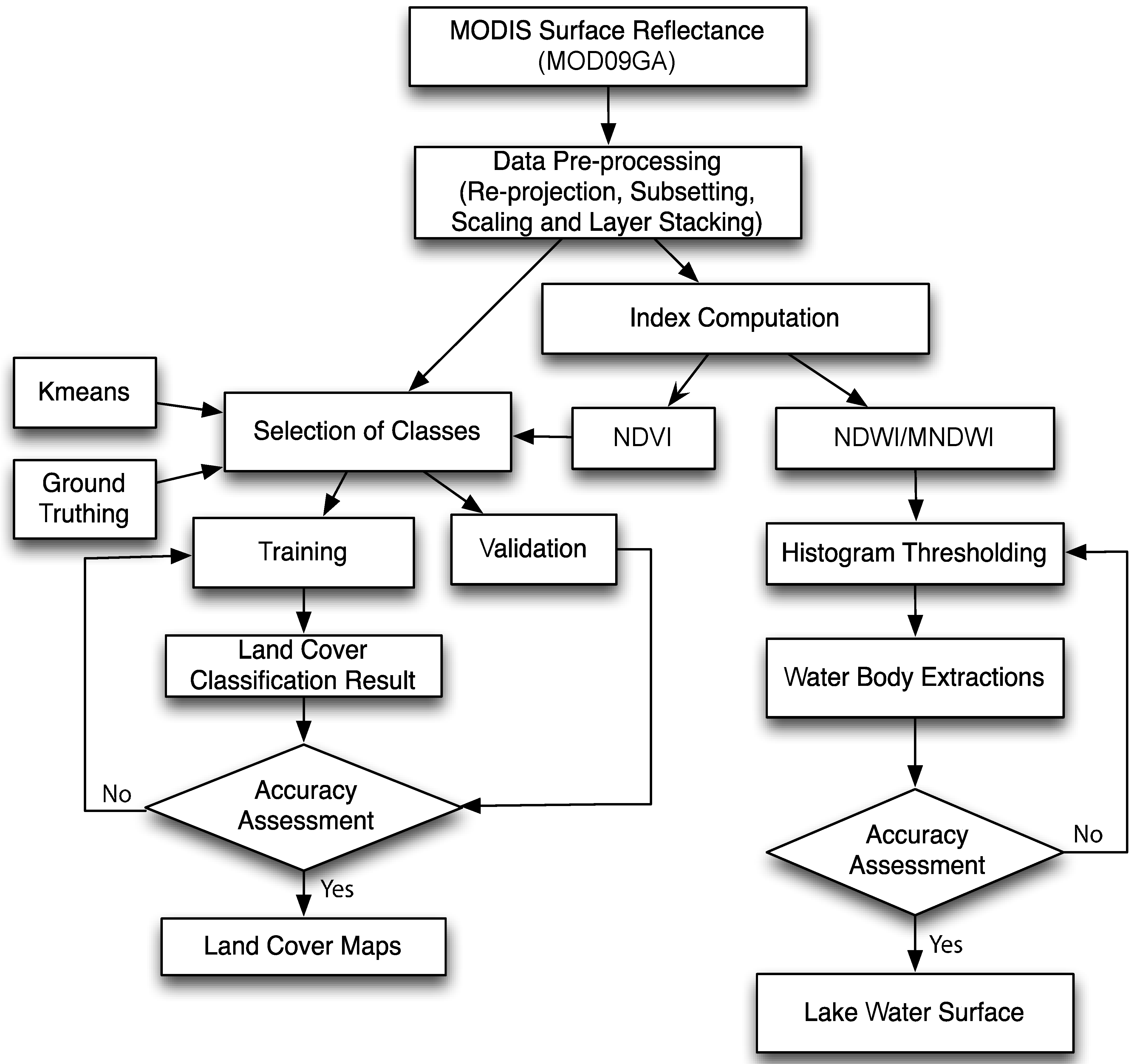
3.2. Lake Water Surface and Land Cover Mapping

All MODIS images were re-projected into UTM projection zone 37 and the World Geodetic System 1984 (WGS84) global reference datum. The data had previously been corrected for radiometric errors and hence is free from atmospheric effects [22]. We applied a scale factor of 0.0001 to all bands in every scene and then stacked them.
We mapped lake water surface dynamics using the index threshold segmentation technique. Threshold segmentation is a fundamental step in extracting water bodies from background [13]. There are several methods which can be applied for image threshold segmentation–histogram shape-based [12,38], clustering-based [39,40,41,42], and entropy-based approaches [43]. We use the histogram-based algorithm to extract water bodies from non-water features. A histogram was generated based on all pixels within the reference lake coastline (Figure 6a). A threshold (T) of the MNDWI was determined from the respective histogram (Figure 6b). For bimodal and multimodal histograms the segmentation threshold was determined by means of Equation (4) [12]:
Water 05 00698 i001
where μWater is the mean value of the water body feature peak, μNon-Water is the mean value of the non-water features peak, and σWater and σNon-Water are their corresponding standard deviations. To map the land cover we used field data and NDVI to identify different classes covering the Lake Manyara catchment. Using NDVI, values between 0 and 0.2 were assigned to a sand/bare soil class, values between 0.2 and 0.3 were categorized as shrubs and grasslands including savannah. Values ranging from 0.3 to 0.6 were assigned to a moderate forest land cover type. This includes savannah, savannah woodland, cropland, natural forest/vegetation and deciduous broad leaf forests. Values between 0.6 and 1 were categorized as dense forest representing mainly evergreen broad leaf forests.
We used a maximum likelihood classification algorithm to map distinguished land cover types in the Manyara catchment. The method is based on both the distances towards class means and the variance-covariance matrix of each class. It groups together features in specified classes based on the likelihood of each feature in the sample set representing a specified class. The technique assumes normality of the training data statistics and assigns pixels to the class with the highest probability value [36]. In this study we performed accuracy assessments in terms of individual error matrices for classified MODIS surface reflectance images generated from maximum likelihood post-classification. We use two main terms to describe the classification accuracy (i.e., overall accuracy and kappa coefficient) [44].
Training sites information for the Maximum likelihood classification was based on field information and on the inspection of spectral profiles (Figure 4). Additionally, the NDVI [34] was employed in order to obtain optimal land cover classes [45]. Since most of the land part of the world is covered by vegetation, using NDVI when performing land cover classification produces more accurate maps [45]. We also use the un-supervised classification k-means algorithm to get impression of the land cover classes. A set of GPS position of polygons were captured for purposes of ground truthing in October/November 2011, a period which is compatible with Lake Manyara’s dry season (June to October/November) within which the MODIS land surface reflectance data were acquired. Data obtained from this fieldwork include GPS position of points and knowledge based information of the study area.
We prepared training and validation sites based on land cover type information, location, size and number of points to be trained for sampling. About 29 sites were selected within the study area and serve as training and testing sites for the Maximum likelihood classification method. The identification of the position of the sampling sites on the images was done based on the field data acquired and NDVI values range. Yet, pixels were inspected for the spectral signatures in order to assure consistency (Figure 4). The trained sites were then divided into two sets; one for classification (training/60% of the sample) and the second was for accuracy assessment (validation/40% of the sample).

3.3. Water Balance Modeling

We used remote sensing data to model Lake Manyara’s water balance from April 2001 to December 2009 using J2000 g hydrological model [46,47]. The model needed two types of input data: temporally varying and constant. The first input is climate data time series and this comprises absolute and relative humidity, sunshine duration, maximum, mean and minimum temperature, wind speed, precipitation and observed runoff. The second input is a set of parameters. These are Hydrological Response Units (HRU) grid-based parameters linked to; (1) land use/land cover such as albedo, stomata conductance (Rsco), maximum plant height (Hmax), leaf area index (LAI), maximum root depth (RDmax) and minimum surface resistance for water-saturated soil; (2) soil thickness and useable field capacity per decimeter of profile depth; (3) the maximum possible percolation rate (ground water recharge rate) per time interval in mm per time unit; (4) mean elevation, slope and aspect. The model was manually calibrated and validated using a novel approach [47]. To calibrate the model, we used initial parameters obtained from a model based on a two month discharge data series. We applied this record to adapt the model parameters as initial calibration parameters for the model that covers the whole study period. After transferring the parameters to the monthly model we adjusted our parameters based on trial and error approach. The model was then validated using two independent datasets; pan evaporation and GRACE based equivalent water thickness data. The validation using observed pan evaporation and simulated evapotranspiration gives a Pearson correlation coefficient, R = 0.83 and the coefficient of determination, r2 = 0.67 [47].

3.4. Possible Sources of Errors

Different sources of errors may affect the accuracy of the extracted water surface and other land cover classes. We computed the class coverage area for different land cover types by multiplying the number of pixels above the defined MNDWI and NDVI thresholds by spatial resolution of MODIS surface reflectance. The area approximations produced by this technique for different dates can vary widely if the images were not corrected radiometrically. Since the surface reflectance value of different land cover classes might be affected by different atmospheric conditions based on their acquisition dates. We omit or reduce all random error caused by these effects due to the fact that the MOD09 land surface reflectance product has been corrected for the effects of atmospheric gases, aerosols, and thin cirrus clouds.
The basic element in a remote sensing satellite data is a pixel. Every pixel consists of spectral reflectance of all objects within a sensors instantaneous field of view. MODIS images have a coarse spatial resolution and are dominated by mixed pixels; particularly pixels covering boundaries between two different land cover classes. In this work we assign each pixel to one single land cover type. For instance we categorized all pixels with NDVI values between 0.2 and 0.3 as grasslands or shrubs. We therefore suspect that the existence of mixed pixels may be another source of random error.
Some of the data used was affected by cloud cover (<10%). To avoid this effect, we assign all cloud cover a single class and exclude it from the analysis by merging all clouds from scenes into a single class and then use this layer as a mask for each image classification process prior to analysis.
MODIS’s medium spatial resolution data are suitable for delineating large vegetation areas and water bodies. However when the lake water level is very shallow, some parts of the water bodies could not be categorized as water and instead they are classified as bare soil or other land cover types. MNDWI classify the water information well [11]. We use the MNDWI to avoid errors caused by miss-identification of shallow water pixels.
Moreover, the hydrologic modeling results obtained in this research contains a certain amount of inherent uncertainties and drawbacks. First, it should be noted that Lake Manyara’s catchment is almost un-gauged. We use in situ climate data measured at the Arusha meteorological station, located near the catchment, in the northeast. The regionalization of the climate data, especially temperature, relative humidity, wind speed and sunshine duration is based on data from one station. Various GIS and remote sensing datasets utilized here have different spatial and temporal resolution. Harmonization of these datasets to the same spatial and temporal resolution requires interpolation and thus introduces errors. The model calibration and validation approach used is adapted due to the lack of in situ data. The trial and error approach for calibration and validation, while common, is not perfect. On the other hand, the use of calibrated data; the robust model chosen and the redundancy of validation data [pan evaporation, gravimetry recovery and climate experiment (GRACE)] indicate that the uncertainties are tolerable for the purpose of this study [47].

4. Results

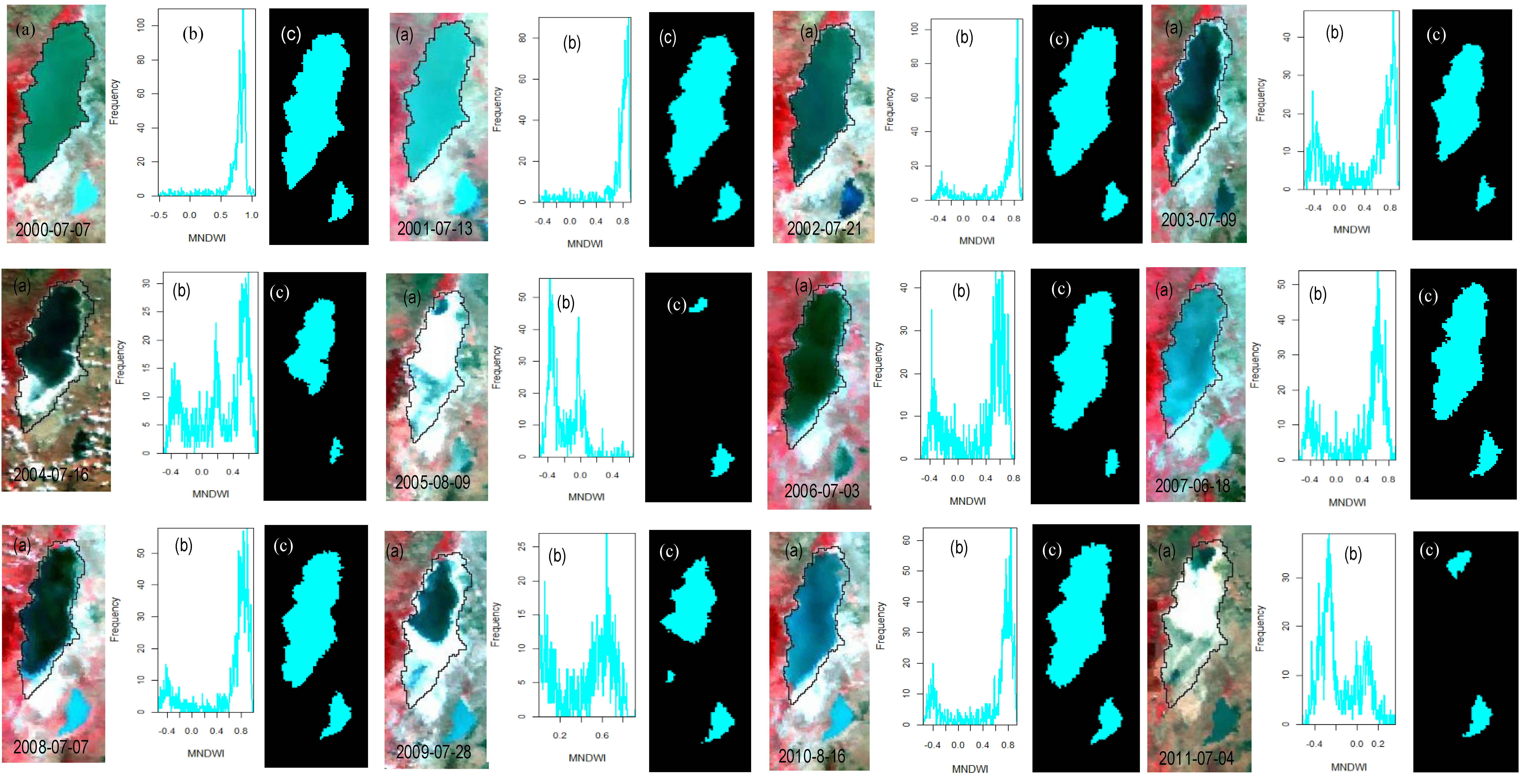
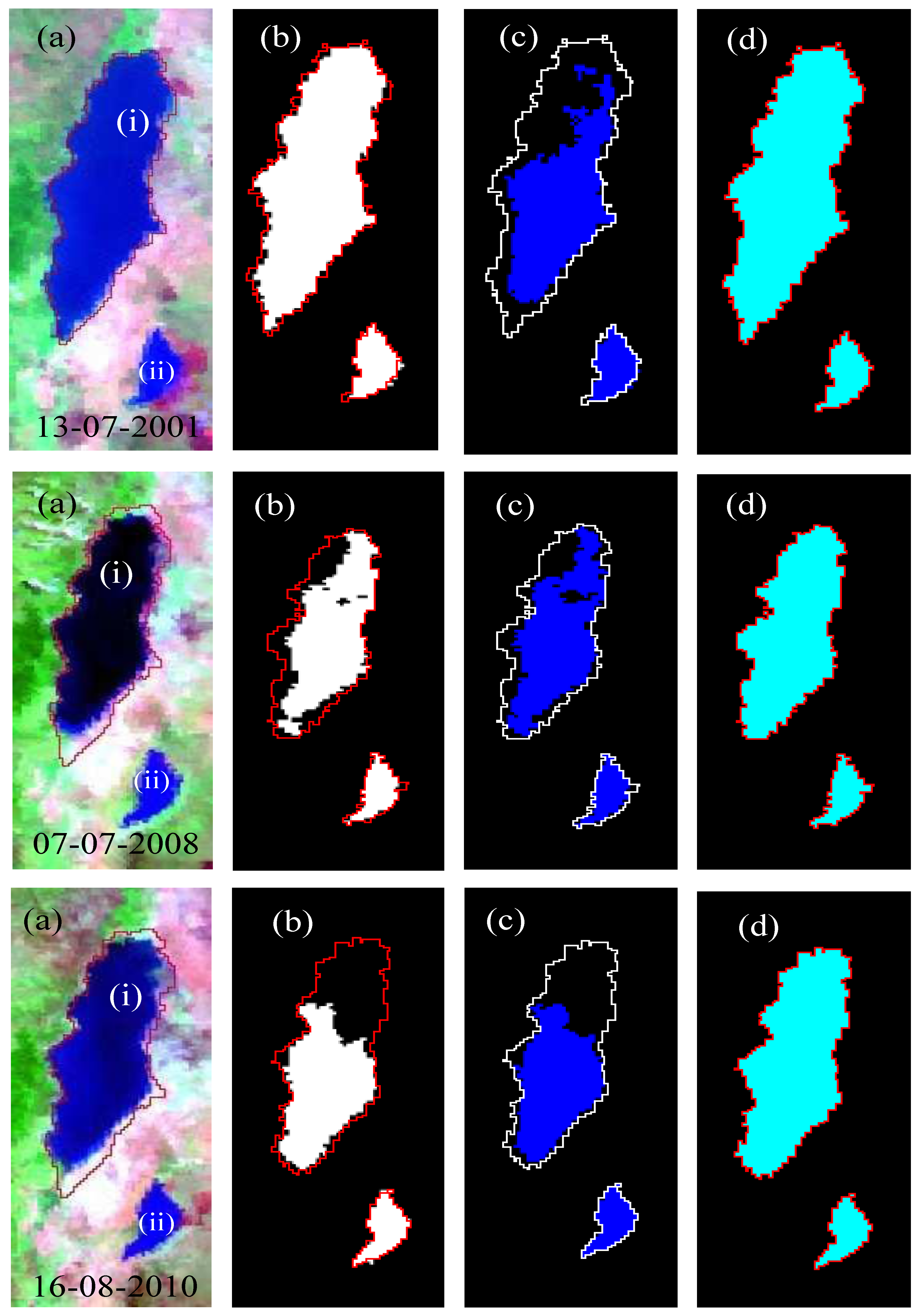
4.1. Lake Manyara Surface Dynamic Mapping

Figure 6 presents the Lake Manyara water surface variation from 2000 to 2011. A subset of MODIS surface reflectance is applied to assess the lake water surface mapping results as (Figure 7) [4]. Table 1 depicts estimated lake water surface dynamic changes, a year-to-year variation (2000–2011) and changes between reference year (i.e., 2000) and respective year. Based on Landsat MSS satellite data the Lake Manyara surface area was 520.50 km2 in September 1973. MODIS surface reflectance data document a lake surface area of 520.25 km2 and 30.5 km2 in July 2000 and July 2011 respectively (Figure 8). High variability of the water surface can be observed for the same month from year to year (Figure 6). The lake water surface area coverage in 2000 was nearly the same as the lake surface area in 1973. The lake water surface area varied significantly during the last decade. The most dramatic lake surface decline was in 2005 and 2011 where the water surface size was 13.25 km2 and 30.5 km2 respectively (Figure 6 and Figure 8).
Figure 8 presents the lake surface area pattern over the last decade in relation to rainfall and air temperature variations. We observe that to some extent the lake surface area depends on rainfall. In 2005 the lake surface dropped considerably, losing about 97.45% of its water surface area. The lake surface increased from 13.25 km2 in 2005 to 383.25 km2 in 2006 following a huge amount of rainfall in 2006.
We assessed monthly variations of the Lake Manyara water surface area in both dry and wet seasons (Figure 9). We compare the lake surface dynamics with mean MNDWI values over the lake and rainfall distribution. The lake water surface area changes with respect to rainfall availability and almost drying out completely during the dry season. The MNDWI depicts a similar trend with the lake water surface coverage.
Figure 6. Lake Manyara surface variation 2000–2011: (a) Lake Manyara MODIS surface Reflectance image subset (RGB band:432) overlayed with lake boundary; (b) Corresponding histogram of the lake pixels (with a peak on the right) within the lake boundary generated using Modified Normalized Difference Water Index (MNDWI); (c) Extracted lake surface using a threshold of 0.
Water 05 00698 g006
Figure 7. Water delineation accuracy assessment (a) Selected MODIS surface reflectance band 432, the image was acquired on 16 August 2010; and (b) The lake demarcation and extraction result of water bodies coastlines as overlaid on the MNDWI map.
Water 05 00698 g007
Table 1. Variation in Lake surface area as extracted from MODIS surface reflectance over the last decade.
YearArea (km2)DurationChange (km2) (%)DurationChange (km2) (%)
2000520.25
20014972000–2001−23.25(4.46)2000–2001−23.25(4.46)
2002451.252001–2002−45.75(9.21)2000–2002−69(13.26)
20033732002–2003−78.25(17.34)2000–2003−147.25(28.30)
20042792003–2004−94(25.20)2000–2004−241.25(46.37)
200513.252004–2005−265.75(95.25)2000–2005−507(97.45)
2006383.252005–2006370(2792.45)2000–2006−137(26.33)
2007449.52006–200766.25(17.29)2000–2007−70.75(13.60)
2008398.252007–2008−51.25(11.40)2000–2008−122(23.45)
2009200.252008–2009−198(49.72)2000–2009−320(61.51)
20104332009–2010232.75(38.05)2000–2010−87.25(16.77)
201130.52010–2011−402.5(92.96)2000–2011−489.75(94.14)
Figure 8. Lake Manyara surface area variation versus annual accumulated rainfall and mean in situ temperature over the catchment.
Water 05 00698 g008
Figure 9. Monthly lake surface area variability as superimposed with monthly average rainfall and temperature patterns, and MNDWI monthly mean series over the lake.
Water 05 00698 g009

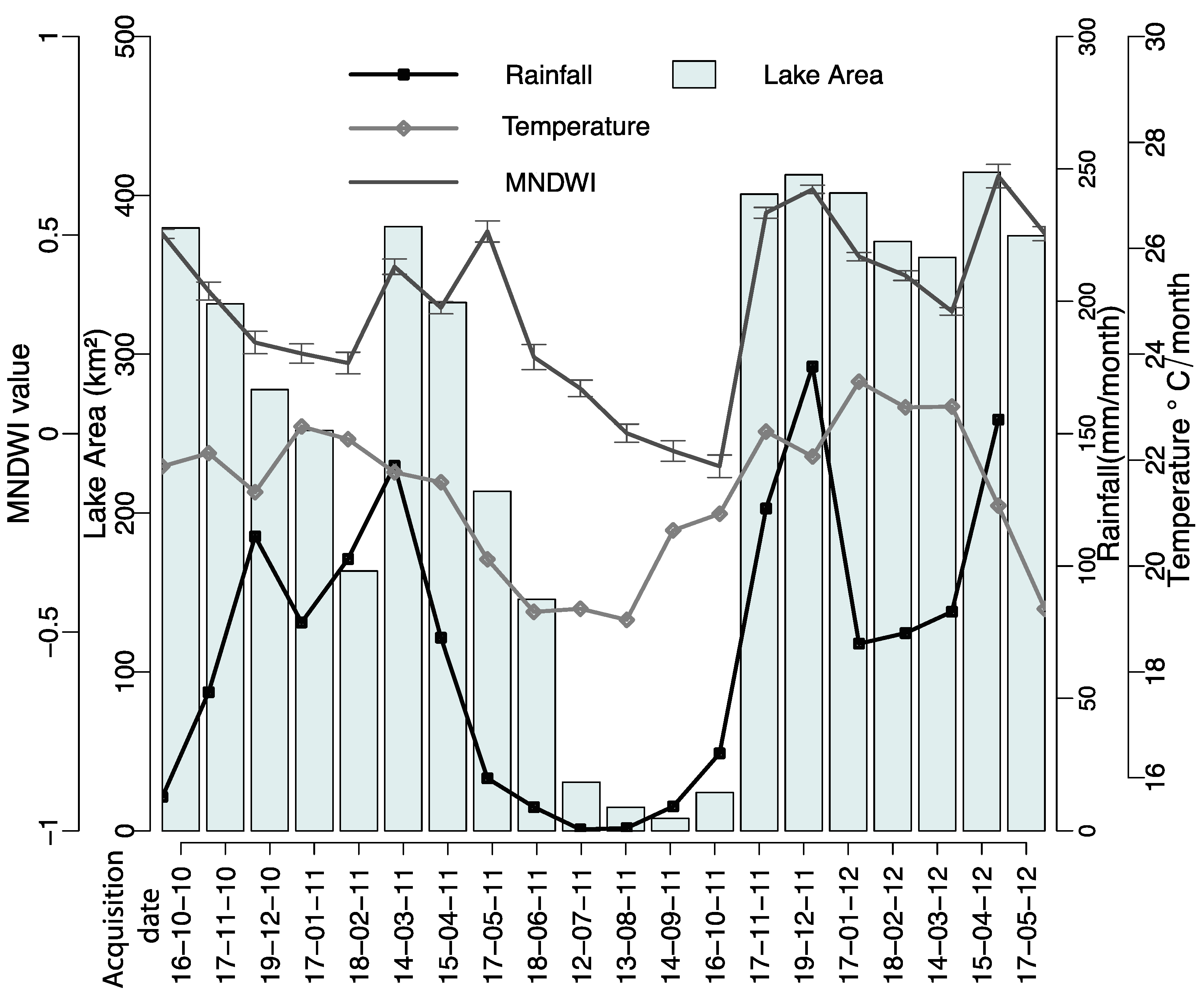
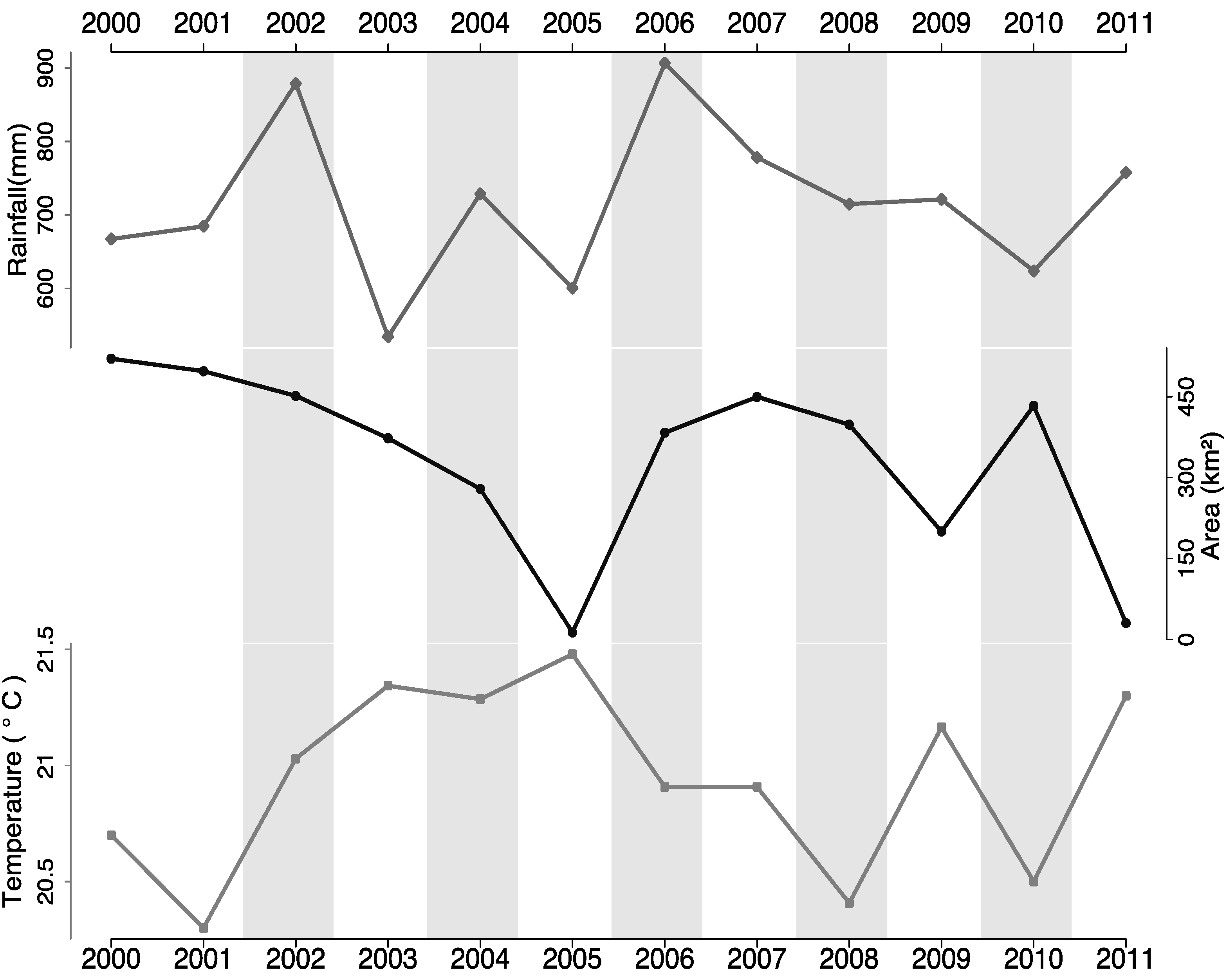
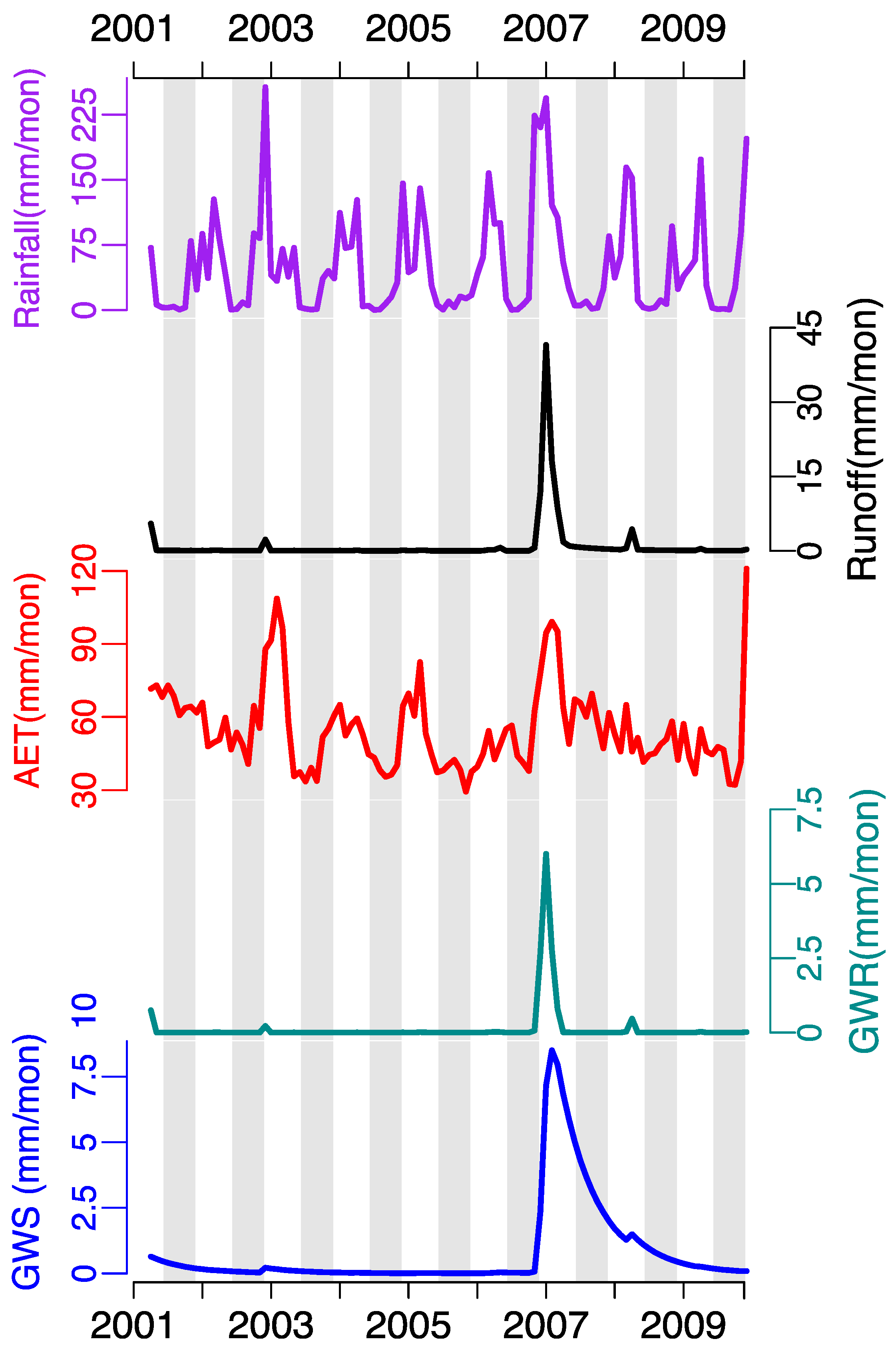
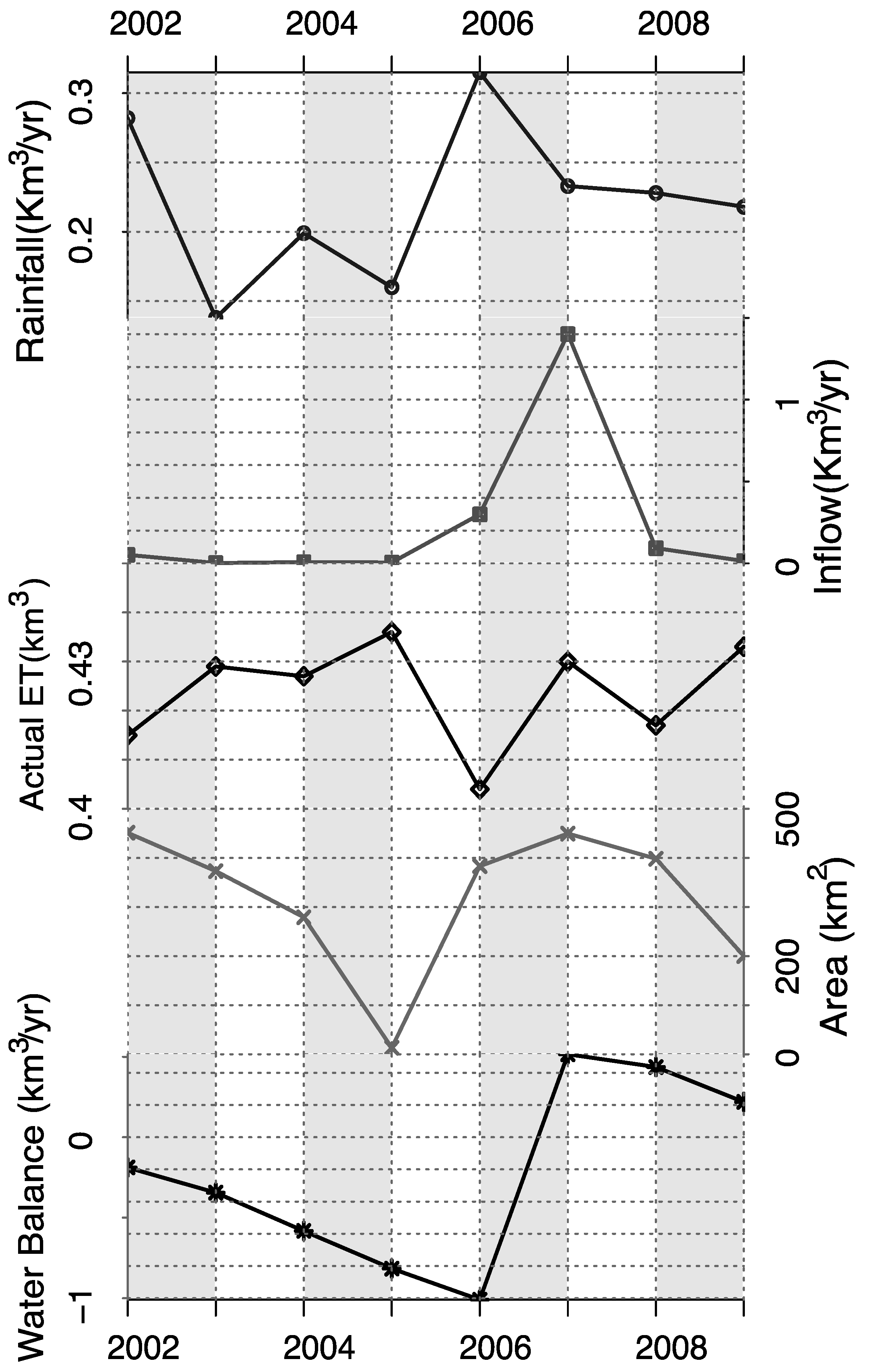
4.2. Water Surface Variations and Water Balance

Figure 10 presents lake Manyara basin monthly distribution of water balance components; precipitation, actual evapotranspiration, runoff and ground water recharge. Figure 11 show simulated lake Manyara’s water balance pattern as compared to lake surface area variation. We also compare the lake water surface variation with MODIS ET and LST time series (Figure 12).
Figure 10. Water balance parameter distribution pattern in Lake Manyara basin from April 2001 to December 2009. GWS stands for ground water storage while GWR is ground water recharge.
Water 05 00698 g010
The water level of Lake Manyara has fluctuated considerably within the last decade. Figure 11 presents Lake Manyara surface water area variations and the annual water balance parameters from 2002 to 2009. We modeled the water balance of the Lake Manyara catchment to study the water cycle using a J2000g semi-distributed hydrological model [46] and remote sensing datasets. We selected the finest calibration parameters for the model based on the Nash-Sutcliffe model efficiency coefficient [48] of 0.60, and a coefficient of determination (r2) of 0.67. The model was validated using pan evaporation and GRACE based equivalent water thickness data. Observed and simulated parameters yielded a Pearson correlation coefficient, R of 0.82 and a coefficient of determination (r2) of 0.7. We estimate the annual mean rainfall over the lake to be 0.22 km3/yr and inflow to the lake as 0.23 km3/yr. Inflow consists of a contribution from streams and underground springs. For the 2002 to 2009 period, rainfall provided approximately 47% of lake water and inflow approximately 53%.
Figure 11. Lake Manyara annual water balance parameters patterns versus lake surface variation.
Water 05 00698 g011
The lake water balance depicts a decreasing trend from 2002 to 2006 and raised considerably in 2007 following an increase of both rainfall and inflow between 2006 and 2007 (Figure 11). We estimate evaporation over the lake to be 0.42 km3/yr between 2002 and 2009 and this accounts for nearly all water loss. We observe a strong relationship between the lake surface variation and lake water balance. In 2007 the lake surface area increased from 383 km2 to 450 km2 while the lake water balance increased from −0.1 km3 to 0.5 km3. The lake surface variation and the water balance display a similar trend from 2006 to 2009.
Figure 12. MODIS evapotranspiration and land surface temperature as displayed with the lake water surface variation from 2002 to 2009.
Water 05 00698 g012

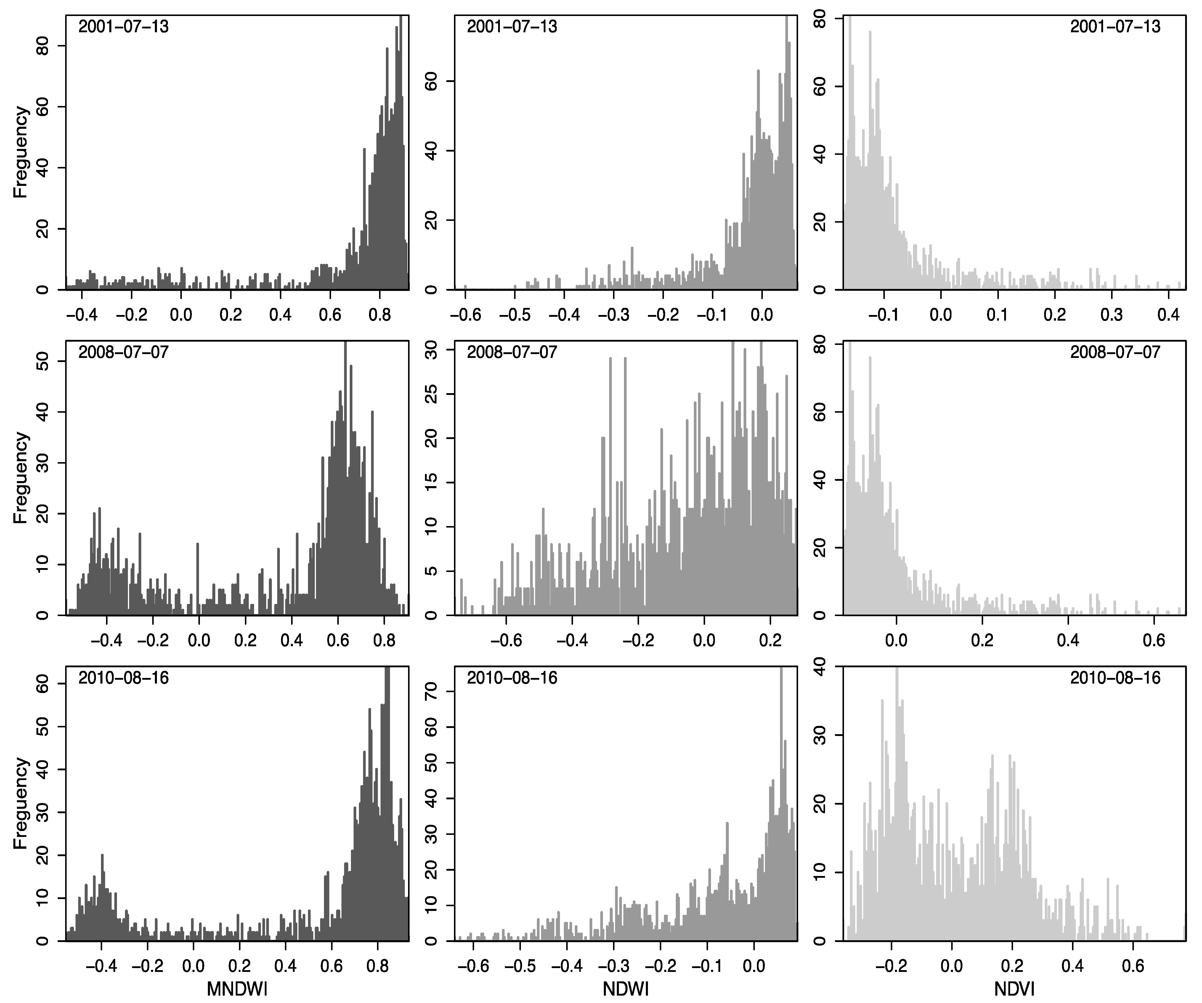
4.3. Assessment of the Optimal Index for Water Extraction

We assessed the performance of MNDWI, NDWI and NDVI in shallow water surface mapping (the case of Lake Manyara) using frequency histograms of the lake pixels within the reference lake coastline (Figure 13, Figure 14). Some of the histograms present a non-symmetric (most of them skewed), bimodal and multi-modal distribution especially for scenes with land/bare soil within the lake body as defined by the reference coastline (Figure 6, Figure 14). For MNDWI and NDWI, water bodies are defined by index values between 0 and 1 [11,14]. The peaks for water bodies are on the right of the plot and those for bare soil are on the left (Figure 14).
The inter-group variances between the lake water area and bare soils are very significant. Intra-group variances are relatively small, particularly for the MNDWI. In Figure 14 the histograms suggest that by means of the MNDWI it is possible to segment the lake water surface accurately using a threshold of 0for all scenes. In most of the images the inter-group variances are not significant for both NDWI and NDVI such that it was not possible to delineate the lake surface using a threshold of 0 (Figure 13).
Figure 13. Index capability comparison. Water bodies extraction in the area of interest using different remote sensing indexes, (i) Lake Manyara and (ii) Lake Burungi; (a) MODIS surface reflectance image subset false color composite band 742 overlaid with lake Manyara coastline as by July 2000; (b)–(d) present water surfaces as delineated using Normalized Difference Vegetation Index (NDVI), Normalized Difference Water Index (NDWI) and MNDWI respectively overlaid with the extracted coastline using MNDWI.
Water 05 00698 g013
Figure 14. Evaluation of MNDWI, NDWI and NDVI performance. Histogram of Lake Manyara pixels [pixels within the reference lake coastline in brown (Figure 13a)] index values by frequency. Lake body peak is on the right side for MNDWI and NDWI, and for NDVI the peak is on the left.
Water 05 00698 g014
Surprisingly, NDVI performed quite well on the scene acquired in July 13, 2001.We suspected that the water level in the lake was high. In May 2010 the Lake Manyara water level was only 1.8 m. Neither NDWI nor NDVI worked well for the image acquired on 16 August 2010 (Figure 13). To evaluate the accuracy of the extracted lake water surface it is necessary to compare the extracted water body coastline with water surface extracted from a ground truth map [49]. Due to the lack of a reliable ground truth map that has been created at least during one acquisition date of the utilized images, we evaluated the lake water surface mapping accuracy by overlaying the MNDWI map with a vector layer of the extracted lake coastlines [4]. We found that they match very well with a mapping accuracy of less than 1 pixel (Figure 14), suggesting that MNDWI is suitable for the extraction of shallow water features [11]. This is also depicted in our monthly lake surface variation analysis (Figure 9) whereby the index depicts a similar trend with the lake water surface dynamics.

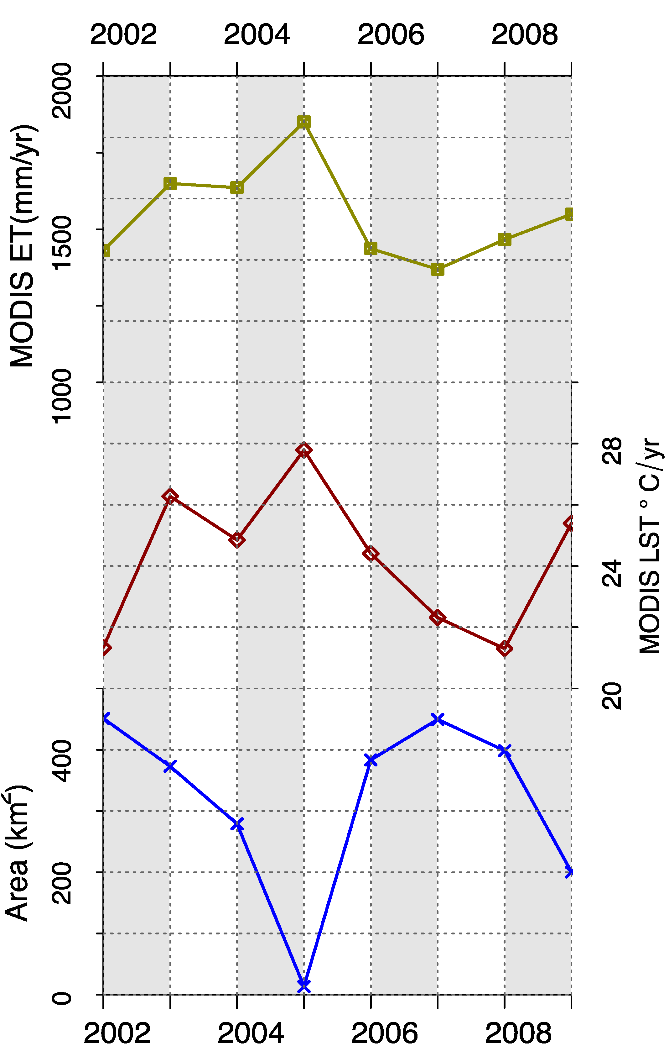
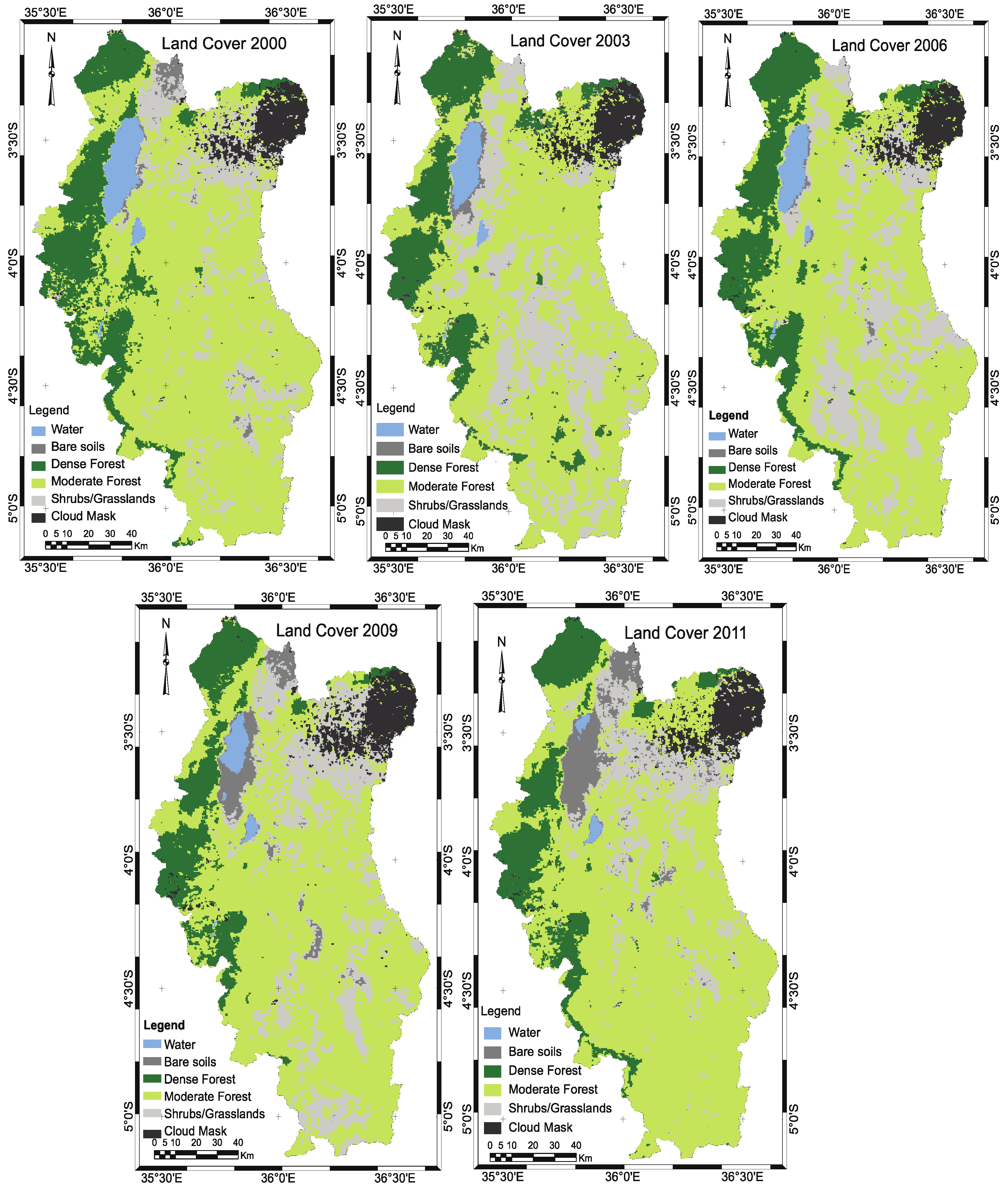
4.4. Land Cover and Lake Surface Area Variation

We chose five MODIS surface reflectance scenes to depict land cover variation within the last decade. Figure 15 presents the spatial distribution of land cover classes within the Lake Manyara basin for 2000, 2003, 2006, 2009 and 2011. We identified five representative land cover classes that were successfully mapped from the satellite imagery. The overall classification accuracy and kappa coefficient for every land cover map is 96% (0.95), 94% (0.92), 88% (0.85), 90% (0.88) and 87% (0.84) respectively. Figure 16 depicts the overall land cover variation pattern in the Manyara basin and accumulated annual rainfall.
Figure 15. Lake Manyara catchment land cover maps 2000–2011.
Water 05 00698 g015
Figure 16. Temporal land cover pattern as overlaid to the catchment annual rainfall distribution.
Water 05 00698 g016

5. Discussion

Our study reveals that the areal extent of the Lake Manyara water surface varied significantly between 2000 and 2011. The water level dropped noticeably in 2005 and rose in 2006 with rainfall being the main contributor (Figure 11). However, alongside rainfall, inflow contributed to the water balance in 2007. The increase of inflow in 2007 was likely a result of high rainfall in 2006. This increased the lake water surface area and the lake water cycle as depicted in Figure 11. We detect that the lake water surface and the lake water balance present a similar trend from 2007 to 2009 (Figure 11). In 2011 the lake water surface dropped markedly (Figure 6, Figure 8). In 2005 and 2011 the lake dried to about 97.45% and 94.14% of the total water surface coverage in 2000 (Table 1). The lake has the potential to completely dry during periods of low rainfall and can then fully recharge following high rainfall events.
We analyzed the relationship between the lake surface area variation and rainfall as the main source of water, temperature and evaporation. The meteorological parameters recorded over the last decade (2000–2011), especially temperature, indicate a generally constant climate with the highest rainfall occurring in 2006 (Figure 8). We observe a correlation between lake surface area fluctuations and rainfall, in situ temperature, actual evaporation, MODIS LST, and MODIS ET (Figure 11, Figure 12). In Figure 12, it can also be perceived clearly that lake Manyara’s storage volume is directly proportional to rainfall, thus lake storage shrinks as the amount of rainfall decreases during dry seasons and expands over rain seasons. This indicates the impact of climate on the lake water cycle. As indicated in Figure 8, Figure 11, Figure 12 in 2005 rainfall was low and the temperature was high, resulting in a large amount of water loss by evaporation. As a result the lake experienced particularly extreme water loss. Heavy rainfall in October 2006 to January 2007 combined with low evaporation due to reduced temperatures resulted in a lake surface water area increase from 13.25 km2 to 383.25 km2 (Table 1, Figure 8, Figure 11). This implies that variation of the lake water surface area is mainly influenced by global and regional climate fluctuations, especially inter annual rainfall variability. We also observe that in 2007, lake surface area increased dramatically (Figure 8, Figure 11) following the occurrences of much rainfall between October 2006 and January 2007. The expansion of lake water surface area as a result of increased rainfall is attributed to the strong positive and negative episodes of Pacific and Indian Ocean sea-surface temperatures (SST) such as El Niño-Southern Oscillation (ENSO) and the Indian Ocean Dipole (IOD) in 2006–2007 [50,51]. Positive IOD and ENSO incidents tend to increase rainfall over east Africa especially in the early segments of the rain season (October–January) [52,53].
We detect the same trend when comparing the lake water surface pattern with MODIS ET and LST time series (Figure 12). We notice that MODIS ET and LST are directly related to each other such that, as LST over the lake increase the ET also increases. Figure 12 shows how the lake water surface area shrank in 2005 as a result of the increase of LST, which was at its highest peak (about 27.8 °C) over the study period. This result in a rise of ET to about 1200 mm/yr. Our evidence suggests that climate fluctuation exerts a dominant control on the fluctuation of the areal extent of Lake Manyara.
However, other factors may affect lake surface dynamics. This includes anthropogenic activities such as irrigation along rivers that feed the lake and natural phenomena like lake water flow to the underground water table. Intensive irrigation activities take place along rivers that drain to Lake Manyara. This releases sediments in the lake basin, which may be one of the reasons for the decline of the water surface. Therefore, in this arid environment, the lake surface variation is to some extent caused by agricultural water consumption [4]. There is a significant withdrawal of water from the streams for irrigation that would otherwise flow into the lake. Nevertheless, estimation of the annual water use for irrigation and livestock in the catchment is not possible currently; it would need an independent study that is out of scope of this work. Figure 17 depicts an irrigation trough along Mto wa Mbu, one of the rivers that flow into Lake Manyara.
However, in our analysis we show that the variation of the lake water surface is primarily a result of the effect of climate variability. We argue that, if the dramatic lake water surface shrinkage were caused mainly by human activities, the lake would have been shrinking at the same rate yearly without following the trends of rainfall and other climatological parameters as indicated in Figure 8, Figure 11, Figure 12. Also taking into account that all utilized images has been acquired in dry season, the period when human activities such as irrigation are supposed to be intensive. It would have been impossible to observe lake surface expansion in some of the years. Therefore, based on our results, we strongly imply that global and regional climate variability is the key cause of lake Manyara water surface fluctuations.
We compared the capabilities of NDVI, NDWI and MNDWI in delineating Lake Manyara’s shallow water surface. NDVI and MNDWI performed quite well in the 2001 image while the NDWI failed to delineate the lake in that particular scene (Figure 13). For the 2008 and 2010 image NDVI and NDWI performed poorly while the MNDWI delineated perfectly the lake water surface area in both scenes (Figure 13). This indicates that MNDWI is suitable for the extraction of water features as suggested by Xu [11]. We successfully used MNDWI to map lake surface dynamics (Figure 6).
Figure 17. (a) An irrigation trough at Mto wa Mbu believed to preclude water from flowing into Lake Manyara; (b) A rice farm irrigated using water from Mto wa Mbu as captured in October 2011.
Water 05 00698 g017
We observe that the distribution of land cover classes is related in all scenes with a moderate forest cover type occupying a large part of the basin over the selected years (Figure 15). The increase of moderated cover vegetation in 2001 is surprising and probably linked to the increase of annual rainfall in 2000 (Figure 16). Moderate forest cover decreased in 2003 following an increase of grassland/shrub cover (Figure 16). Shrub/grasslands increased in 2009 and 2010 while moderate forest cover decreased during this time (Figure 16). The trend of lake water surface area, dense and moderate forest cover degradation and regrowth is directly related to fluctuations in annual rainfall (Figure 16). Dense and moderate forest cover increases as shrubs/grasslands decrease (Figure 16). We did not observe any relationship between land cover variation in the catchment and the lake surface area variations from 2000 to 2011 (Figure 16). Therefore, we conclude that lake surface variation is not directly related to the type of land cover classes in the catchment (Figure 16).

Implication to Water Resource Management

Water resources data are prerequisite for resource planning, design, operation and conservation [54]. Optimized monitoring of water resources status patterns for example, is a key factor for effective and sustainable water resource management. In African semi-arid areas, water resources data, despite being fundamentally important has not been given the attention it deserves, such that implementation of water resource management programs and policies is constrained due lack of timely and up to date information. Our ability to manage water resources efficiently for sustainable utilization is hampered by a lack of understanding of the state of the water resource and trends.
Over the past two decades, remote sensing has shown promising results in estimation of water storage in large reservoirs and lakes [3]. However, in this study we show a simplest way to assess and obtain water resource surface state dynamics for smaller and shallow lakes. Smaller and shallow lakes are main sources of water in Africa and semi-arid environments, such that they must be managed and conserved sustainably.
Assessments of water resources are becoming increasingly important especially in the time of rapidly human induced climatic fluctuation that results in higher variability of water resources over the globe. Water resource dynamics maps provide visual impression of the fluctuations of water resources on both spatial and temporal coverage to decision and policy makers and to water resource managers. Water resource assessment and monitoring therefore, provides the means to understand the state of the water resource, hence could facilitate timely decision on the magnitude of the effort required for protection thereafter, improved water resource management.

6. Conclusions

In this study we show the potential of remote sensing in water resource status dynamics assessment and monitoring. Our study shows that Lake Manyara has experienced a significant surface area variation from 2000 to 2011, and almost dried completely in 2005 and 2011. We detect that the lake surface area has been decreasing since 2000. The lake surface variation and the lake hydrological cycle water balance pattern displayed a similar trend from 2006 and 2007. The trend of decreasing lake surface area portrays a strong relationship with the distribution of meteorological parameters indicating a strong impact of climate on the lake. We conclude that the lake water surface is dominantly influenced by inter annual variability in rainfall, as influenced by global and regional climate fluctuations. Anthropogenic activities adjacent to rivers that feed the lake are likely an additional factor that requires further investigation.
We demonstrate that MNDWI is most suitable and easiest technique for the delineation and mapping of water resources even shallow and smaller water bodies. Generally, our results show that remote sensing is an efficient method for assessing water resources in semi-arid environments. Specifically, we conclude that TRMM, MODIS surface reflectance, ET, and LST remote sensing based datasets provide great potential for the mapping and monitoring of water resources. We suggest that, the method employed in this research should be applied to assess and monitor water resource status dynamics in semi-arid environments provided the availability of satellite datasets. Thereafter, required water resource information by policy/decision makers and water resource managers will be acquired and hence optimized sustainable management and conservation.

Acknowledgements

We would like to acknowledge the financial support of the German Academic Exchange Service (DAAD) to Dorothea Deus for her Ph.D. research project at Freiberg University of Mining and Technology, Germany. We are greatly indebted to the U.S. Geological Survey (USGS) for providing us with MOD09GA and MCD43A4; the MODIS surface reflectance product, TRMM rainfall product used in this study were acquired using the GES-DISC Interactive Online Visualization ANd aNalysis Infrastructure (Giovanni) as part of the NASA’s Goddard Earth Sciences (GES) Data and Information Services Center (DISC). We also express our sincere gratitude to Adam Szulc for proofreading the article.

Conflicts of Interest

The author declares no conflict of interest.

References

  1. Birol, E.; Karousakis, K.; Koundouri, P. Using economic valuation techniques to inform water resources management: A survey and critical appraisal of available techniques and an application. Sci. Total Environ. 2006, 365, 105–122. [Google Scholar] [CrossRef]
  2. Chave, P. The EU Water Framework Directive: An Introduction; IWA Publishing: London, UK, 2001; p. 208. [Google Scholar]
  3. Gao, H.; Birkett, C.; Lettenmaier, D.P. Global monitoring of large reservoir storage from satellite remote sensing. Water Resour. Res. 2012, 48, W09504:1–W09504:12. [Google Scholar]
  4. Bai, J.; Chen, X.; Li, J.; Yang, L.; Fang, H. Changes in the area of inland lakes in arid regions of central Asia during the past 30 years. Environ. Monit. Assess. 2011, 178, 247–256. [Google Scholar] [CrossRef]
  5. Mason, I.M.; Guzkowska, M.A.J.; Rapley, C.G. The response of lake levels and areas to climatic change. Clim. Change 1994, 27, 161–197. [Google Scholar] [CrossRef]
  6. Mercier, F.; Cazenave, A.; Maheu, C. Interannual lake level fluctuations (1993–1999) in Africa from Topex/Poseidon: Connections with ocean-atmosphere interactions over the Indian Ocean. Glob. Planet. Change 2002, 32, 141–163. [Google Scholar] [CrossRef]
  7. Goerner, A.; Jolie, E.; Gloaguen, R. Non-climatic growth of the saline Lake Beseka, Main Ethiopian Rift. J. Arid Environ. 2009, 73, 287–295. [Google Scholar] [CrossRef]
  8. Verbesselt, J.; Hyndman, R.; Newnham, G.; Culvenor, D. Detecting trend and seasonal changes in satellite image time series. Remote Sens. Environ. 2010, 114, 106–115. [Google Scholar]
  9. Crétaux, J.; Jelinski, W.; Calmant, S.; Kouraev, A.; Vuglinski, V.; Bergé-Nguyen, M.; Gennero, M.-C.; Nino, F.; Abarca Del Rio, R.; Cazenave, A.; et al. SOLS: 2011. A lake database to monitor in the Near Real Time water level and storage variations from remote sensing data. Adv. Space Res. 2011, 47, 1497–1507. [Google Scholar] [CrossRef]
  10. Böhme, B.; Steinbruch, F.; Gloaguen, R.; Heilmeier, H.; Merkel, B. Geomorphology, hydrology, and ecology of Lake Urema, central Mozambique, with focus on lake extent changes. Phys. Chem. Earth 2006, 31, 745–752. [Google Scholar] [CrossRef]
  11. Xu, H. Modification of normalised difference water index (NDWI) to enhance open water features in remotely sensed imagery. Int. J. Remote Sens. 2006, 27, 3025–3033. [Google Scholar] [CrossRef]
  12. Li, J.; Sheng, Y. An automated scheme for glacial lake dynamics mapping using Landsat imagery and digital elevation models: A case study in the Himalayas. Int. J. Remote Sens. 2012, 33, 5194–5213. [Google Scholar]
  13. Lu, S.; Wu, B.; Yan, N.; Wang, H. Water body mapping method with HJ-1A/B satellite imagery. Int. J. Appl. Earth Observ. Geoinf. 2011, 13, 428–434. [Google Scholar] [CrossRef]
  14. McFeeters, S.K. The use of normalized difference water index (NDWI) in the delineation of open water features. Int. J. Remote Sens. 1996, 17, 1425–1432. [Google Scholar] [CrossRef]
  15. Luo, J.; Sheng, Y.; Shen, Z.; Li, J. Automatic and high-precise extraction for water in- formation from multispectral images with the step-by-step iterative transformation mechanism. J. Remote Sens. 2009, 13, 604–609. [Google Scholar]
  16. Simonsson, L. Applied Landscape Assessment in a Holistic Perspective, A Case Study from Babati District, North-Central Tanzania; Department of Earth Science, Uppsala University: Uppsala, Sweden, 2001; pp. 1650X–1495X. [Google Scholar]
  17. Yanda, P.Z.; Madulu, N.F. Water resource management and biodiversity conservation in the Eastern Rift Valley Lakes, Northern Tanzania. Phys. Chem. Earth 2005, 30, 717–725. [Google Scholar] [CrossRef]
  18. Kaspar, F.; Cubasch, U.; Offenbach, G. Simulation of East African precipitation patterns with the regional climate model CLM. Meteorol. Z. 2008, 17, 511–517. [Google Scholar] [CrossRef]
  19. Khan, S.I.; Adhikari, P.; Hong, Y.; Vergara, H.; Adler, R.F.; Policelli, F.; Irwin, D.; Korme, T.; Okello, L. Hydroclimatology of Lake Victoria region using hydrologic model and satellite remote sensing data. Hydrol. Earth Syst. Sci. 2011, 15, 107–117. [Google Scholar] [CrossRef]
  20. Copeland, S.R. Potential hominin plant foods in northern Tanzania: Semi-arid savannas versus savanna chimpanzee sites. J. Hum. Evol. 2009, 57, 365–378. [Google Scholar] [CrossRef]
  21. Prins, H.T.; Loth, P.E. Rainfall patterns as background to plant phenology in northern Tanzania. J. Biogeogr. 1988, 15, 451–463. [Google Scholar] [CrossRef]
  22. Vermote, E.F.; Kotchenova, S.Y.; Ray, J.P. MODIS Land Surface Reflectance User Guide V1.3. 2011. Available online: http://modis-sr.ltdri.org/products/MOD09_UserGuide_v1_3.pdf (accessed on 30 September 2012).
  23. Schaaf, C.B.; Gao, F.; Strahler, A.H.; Lucht, W.; Li, X.; Tsang, T.; Strugnell, N.; Zhang, X.Y.; Jin, Y.; Muller, J.P.; et al. First operational BRDF, albedo and nadir reflectance products from MODIS. Remote Sens. Environ. 2002, 83, 135–148. [Google Scholar] [CrossRef]
  24. Wan, Z. New refinements and validation of the MODIS land-surface temperature/emissivity products. Remote Sens. Environ. 2008, 112, 59–74. [Google Scholar] [CrossRef]
  25. Sun, Z.; Wang, Q.; Ouyang, Z.; Watanabe, M.; Matsushita, B.; Fukushima, T. Evaluation of MOD16 algorithm using MODIS and ground observational data in winter wheat field in North China Plain. Hydrol. Process. 2007, 21, 1196–1206. [Google Scholar] [CrossRef]
  26. Mu, Q.; Heinsch, F.A.; Zhao, M.; Running, S.W. Development of a global evapotranspiration algorithm based on MODIS and global meteorology data. Remote Sens. Environ. 2007, 111, 519–536. [Google Scholar] [CrossRef]
  27. Mu, Q.; Zhao, M.; Running, S.W. Improvements to a MODIS global terrestrial evapotranspiration algorithm. Remote Sens. Environ. 2011, 115, 1781–1800. [Google Scholar] [CrossRef]
  28. Oak Ridge National Laboratory Distributed Active Archive Center (ORNL DAAC), MODIS Subsetted Land Products, Collection 5. Oak Ridge, TN, USA, 2012. Available online: http://daac.ornl.gov/MODIS/modis.html (accessed on 31 August 2012).
  29. Bookhagen, B.; Burbank, D.W. Toward a complete Himalayan hydrological budget: Spatiotemporal distribution of snowmelt and rainfall and their impact on river discharge. J. Geophys. Res. 2010, 115, F03019:1–F03019:25. [Google Scholar]
  30. Kim, H.W.; Hwang, K.; Mu, Q.; Lee, O.S.; Choi, M. Validation of MODIS 16 global terrestrial evapotranspiration products in various climates and land cover types in Asia. KSCE J. Civil Eng. 2012, 16, 229–238. [Google Scholar] [CrossRef]
  31. Tang, R.; Li, Z.; Chen, K. Validating MODIS–derived land surface evapotranspiration with in situ measurements at two AmeriFlux sites in a semiarid region. J. Geophys. Res. 2011, 116, D04106:1–D04106:14. [Google Scholar]
  32. Kummerow, C.; Barnes, W.; Kozu, T.; Shiue, J.; Simpson, J. The tropical rainfall measuring mission (TRMM) sensor package. J. Atmos. Ocean. Technol. 1998, 15, 809–817. [Google Scholar] [CrossRef]
  33. Huffman, G.J.; Adler, R.F.; Bolvin, D.T.; Gu, G.J.; Nelkin, E.J.; Bowman, K.P.; Hong, Y.; Stocker, E.F.; Wolff, D.B. The TRMM multisatellite precipitation analysis (TMPA): Quasiglobal, multiyear, combined-sensor precipitation estimates at fine scales. J. Hydrometeorol. 2007, 8, 38–55. [Google Scholar] [CrossRef]
  34. Rousel, J.W.; Haas, R.H.; Schell, J.A.; Deering, D.W. Monitoring vegetation systems in the great plains with ERTS. In Proceedings of the Third Earth Resources Technology Satellite—1 Symposium; NASA SP-351; NASA: Greenbelt, MD, USA, 1974; Volume 1, pp. 309–317. [Google Scholar]
  35. Soti, V.; Tran, A.; Bailly, J.; Puech, C.; Seen, D.L.; Bégué, A. Assessing optical earth observation systems for mapping and monitoring temporary ponds in arid areas. Int. J. Appl. Earth Observ. Geoinf. 2009, 11, 344–351. [Google Scholar] [CrossRef] [Green Version]
  36. Jensen, J.R. Introductory to Digital Image Processing: A Remote Sensing Perspective, 3rd ed.; Prentice Hall Press: Upper Saddle River, NJ, USA, 2005. [Google Scholar]
  37. Sobrino, J.A.; Raissouni, N. Toward remote sensing methods for land cover dynamic monitoring: Application to Morocco. Int. J. Remote Sens. 2000, 21, 353–366. [Google Scholar] [CrossRef]
  38. Glasbey, C.A. An analysis of histogram-based thresholding algorithms. Graph. Models Image Process. 1993, 55, 532–537. [Google Scholar] [CrossRef]
  39. Cheriet, M.; Said, J.N.; Suen, C.Y. A recursive thresholding technique for image segmentation. IEEE Trans. Image Process. 1988, 7, 918–921. [Google Scholar] [CrossRef]
  40. Jawahar, C.V.; Biswas, P.K.; Ray, A.K. Investigations on fuzzy thresholding based on fuzzy clustering. Pattern Recognit. 1997, 30, 1605–1613. [Google Scholar] [CrossRef]
  41. Otsu, N. A threshold selection method from grey-level histograms. IEEE Trans. Syst. Man Cybernet. 1979, 9, 62–66. [Google Scholar] [CrossRef]
  42. Tizhoosh, H.R. Image thresholding using type II fuzzy sets. Pattern Recognit. 2005, 38, 2363–2372. [Google Scholar] [CrossRef]
  43. Cheng, H.D.; Chen, Y.H.; Sun, Y. A novel fuzzy entropy approach to image enhancement and thresholding. Signal Process. 1999, 31, 745–752. [Google Scholar]
  44. Congalton, R.G.; Green, K. Assessing the Accuracy of Remotely Sensed Data: Principles and Practices; CRR/Lewis Publishers: Boca Raton, FL, USA, 1999; p. 137. [Google Scholar]
  45. Knight, J.F.; Lunetta, R.L.; Ediriwickrema, J.; Khorram, S. Regional scale land-cover characterization using MODIS-NDVI 250 m multi-temporal imagery: A phenology based approach. GISci. Remote Sens. 2006, 43, 1–23. [Google Scholar]
  46. Krause, P.; Hanisch, S. Simulation and analysis of the impact of projected climate change on the spatially distributed waterbalance in Thuringia, Germany. Adv. Geosci. 2009, 21, 33–48. [Google Scholar] [CrossRef]
  47. Deus, D.; Gloaguen, R.; Krause, P. Water balance modeling in a semi-arid environment with limited in situ data using remote sensing in Lake Manyara, East African Rift, Tanzania. Remote Sens. 2013, 5, 1651–1680. [Google Scholar] [CrossRef]
  48. Nash, J.E.; Sutcliffe, J.V. River flow forecasting through conceptual models. Part I: A discussion of principles. J. Hydrol. 1970, 10, 282–290. [Google Scholar] [CrossRef]
  49. Alesheikh, A.A.; Ghorbanali, A.; Nbouri, N. Coastline change detection using remote sensing. Int. J. Environ. Sci. Technol. 2007, 4, 61–66. [Google Scholar]
  50. Abram, N.J.; Gagan, M.K.; Liu, Z.; Hantoro, W.S.; McCulloch, M.T.; Suwargadi, B. Seasonal characteristics of the Indian Ocean Dipole during the Holocene epoch. Nature 2007, 445, 299–302. [Google Scholar]
  51. Paeth, H.; Hense, A. On the linear response of tropical African climate to SST changes deduced from regional climate model simulations. Theor. Appl. Climatol. 2006, 83, 1–19. [Google Scholar] [CrossRef]
  52. Schreck, C.J.; Semazzi, F.H. Variability of the recent climate of eastern Africa. Int. J. Climatol. 2004, 24, 681–701. [Google Scholar] [CrossRef]
  53. Ummenhofer, C.C.; Gupta, A.S.; England, M.H.; Reason, C.J.C. Contributions of Indian Ocean sea surface temperatures to enhanced East African rainfall. J. Climatol. 2009, 22, 993–1013. [Google Scholar] [CrossRef]
  54. Donkor, S.M.K.; Wolde, Y.E. Intergrated Water Resource Management in Africa: Issues and Options. Available online: http://www.gdrc.org/uem/water/iwrm/iwrm-africa.pdf (accessed on 12 December 2012).

