Wetland Monitoring Using the Curvelet-Based Change Detection Method on Polarimetric SAR Imagery

Abstract

One fundamental task in wetland monitoring is the regular mapping of (temporarily) flooded areas especially beneath vegetation. Due to the independence of weather and illumination conditions, Synthetic Aperture Radar (SAR) sensors could provide a suitable data base. Using polarimetric modes enables the identification of flooded vegetation by means of the typical double-bounce scattering. In this paper three decomposition techniques—Cloude-Pottier, Freeman-Durden, and Normalized Kennaugh elements—are compared to each other in terms of identifying the flooding extent as well as its temporal change. The image comparison along the time series is performed with the help of the Curvelet-based Change Detection Method. The results indicate that the decomposition algorithm has a strong impact on the robustness and reliability of the change detection. The Normalized Kennaugh elements turn out to be the optimal representation for Curvelet-based change detection processing. Furthermore, the co-polarized channels (same transmit and receive polarization in horizontal (HH) and vertical (VV) direction respectively) appear to be sufficient for wetland monitoring so that dual-co-polarized imaging modes could be an alternative to conventional quad-polarized acquisitions.

1. Introduction

Synthetic Aperture Radar (SAR) remote sensing has shown a high potential in surveying flood events [1,2]. Smooth water surfaces can easily be detected by their very low backscattering value: the transmitted radiation is almost completely scattered away from the sensor. For rougher water surfaces—induced by wind or currents—the backscattering might increase significantly so that more sophisticated methods have to be applied [3]. Another challenge in the context of wetland monitoring is the detection of water beneath vegetation canopies. Using optical sensors there is no chance to penetrate leaves and branches. Thus, densely forested areas will always appear green independent of the flood situation on ground. With SAR sensors—operating in much longer wavelengths—the radiation penetrates the canopy and images underlying objects as well [4]. As simple SAR intensity images cannot distinguish where the signal received comes from—canopy or ground—multi-polarized SAR mode are required. This type of SAR images allows the discrimination of different backscattering mechanisms. In general, following three scattering types are addressed:

• Surface scattering—a target, that is rough enough to reflect transmitted radiation, but still smooth in relation to the wavelength (about 5cm for RADARSAT-2);
• Diplane scattering—a so-called double-bounce effect occurring when two perpendicular planes are imaged and thus, the radiation is reflected twice before reception;
• Volume scattering—a purely diffuse backscattering behavior caused by a huge number of disordered dipoles, e.g., inside a backscattering object or volume.

Volume scattering can mainly be found in tree crowns, while surface scattering can be attached to bare soil or the canopy dependent on leave size, density, etc. Double-bounce scattering is rare in natural environments in default of perpendicular backscattering planes. But, it occurs as soon as vegetation—grass or even trees—is flooded and the culms or trunks respectively form a diplane target in conjunction with the water surface. Thus, open water can be detected by its low backscattering—in all channels—and flooded vegetation appears as high backscattering in the diplane channel of a polarimetric decomposition.

Former studies use this high contrast in the backscattering strength for moisture estimation out of single-polarized data [5]. Others utilize flooded vegetation as strong deterministic scatterer that raises and lowers with the water level and therefore modifies the observed interferometric phase [6]. This requires stable backscattering throughout the observation period and relatively small water level changes. A multi-polarized attempt is reported in [7] where the amplitudes in horizontal and vertical polarization, but no phase information, are interpreted and correlated with certain wetland characteristics. A good overview of SAR wetland monitoring is given in [8]. Although the inclusion of optical data sets as well was evaluated and revealed significant synergistic effects in former studies [9], this paper will focus on SAR data only because of the all-weather capability of space-borne SAR sensors. The polarimetric signal will be evaluated in terms of amplitude and phase information.

In order to monitor the temporal change of a wetland by the help of polarimetric SAR data there are two basic methods: first, classify each scene—e.g., by correlating wetland categories and scattering mechanisms [10]—and then compare the classification results and second, extract and interpret changes by comparing two images directly. As the reliability of the first method announced always is restricted by the drawbacks of the classification algorithms used, we decided to follow the second approach. As input for the change detection the output layers of three different polarimetric decompositions are chosen. Instead of a pixel-wise comparison the image differences and quotients respectively are calculated and subsequently enhanced in the Curvelet coefficient domain. This procedure is known to deliver robust and reliable results by suppressing small-scale and un-structured noise [2,11].

The objective of this study was to evaluate the Freeman-Durden and Cloude-Pottier decompositions along with the Normalized Kennaugh elements for wetland monitoring applications and change detection in order to find an optimal decomposition for robust change detection that might be transferred to data acquired by other SAR sensors as well. The combination of the Curvelet-based change detection which is known to be robust against noise and very sensitive towards structures and the Normalized Kennaugh Elements seems most promising because of the flexibility of the Kennaugh element description with respect to varying acquisitions modes of SAR sensors. The following sections describe the study area, the methodology used in the study, as well as the results of the three different approaches and discuss implications for this application.

2. Study Area

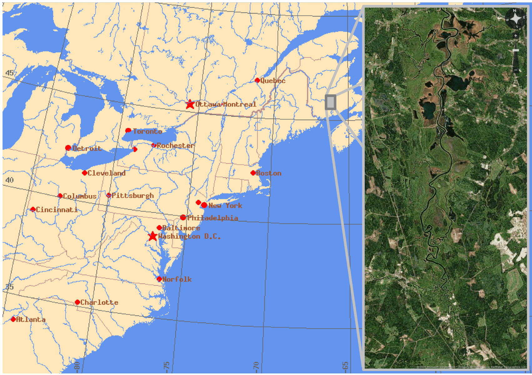
The Gagetown, New Brunswick site is in north central New Brunswick with a climate marked by warm summers and mild, snowy winters. The mean annual temperature is approximately 5 °C. The mean summer temperature is 15.5 °C and the mean winter temperature is −5.5 °C. The mean annual precipitation ranges 900–1300 mm. The lowlands are underlain by flat to gently dipping sandstones, shales, and conglomerates and rise inland from sea level to 200 m. The region is blanketed with moraine. The dominant soils are Humo Ferric Podzols and Gray Luvisols with significant areas of Gleysols, Fibrisols and Mesisols on wetter sites. The closed mixed wood forest is mainly composed of red spruce, balsam fir, red maple, hemlock, and eastern white pine. Sugar maple and yellow birch are found on the larger hills. Wetlands are extensive and support dwarf black spruce and eastern larch at their perimeters. Low density river and stream networks prevail, flowing into the Northumberland and St. Lawrence Gulf areas. Figure 1 shows the location of the Gagetown site as well as an optical image.

3. Methodology

The methodology comprises three sections: a data description, the polarimetric decompositions, and the change detection. In the last two sections the algorithms used in this study are briefly introduced and references are given—where possible—for more detailed description.

Figure 1. Location map (EOWEB^®) and optical image (©2009 Microsoft Corporation, Redmond, WA, USA; Imagery © Harris Corp, Melbourne, FL, USA; Earthstar Geographics LLC, San Diego, CA, USA; NAVTEQ, Chicago, IL, USA) of the study area near Gagetown, New Brunswick, Canada.

Figure 1. Location map (EOWEB^®) and optical image (©2009 Microsoft Corporation, Redmond, WA, USA; Imagery © Harris Corp, Melbourne, FL, USA; Earthstar Geographics LLC, San Diego, CA, USA; NAVTEQ, Chicago, IL, USA) of the study area near Gagetown, New Brunswick, Canada.

3.1. Data Description

Multi-temporal RADARSAT-2 (Data and Product © Macdonald, Dettwiler and Associates Ltd., Richmond, BC, Canada, 2010) FineQuad acquisitions over a wetland near Gagetown, NB, Canada are used in this study. The images date from 27 April, 21 May, 14 June, 8 July, and 1 August of the year 2010. They all share the same acquisition geometry with an incidence angle of about 36° and have been geocoded with a pixel spacing of 4 m by the help of the SRTM elevation model before polarimetric decomposition. 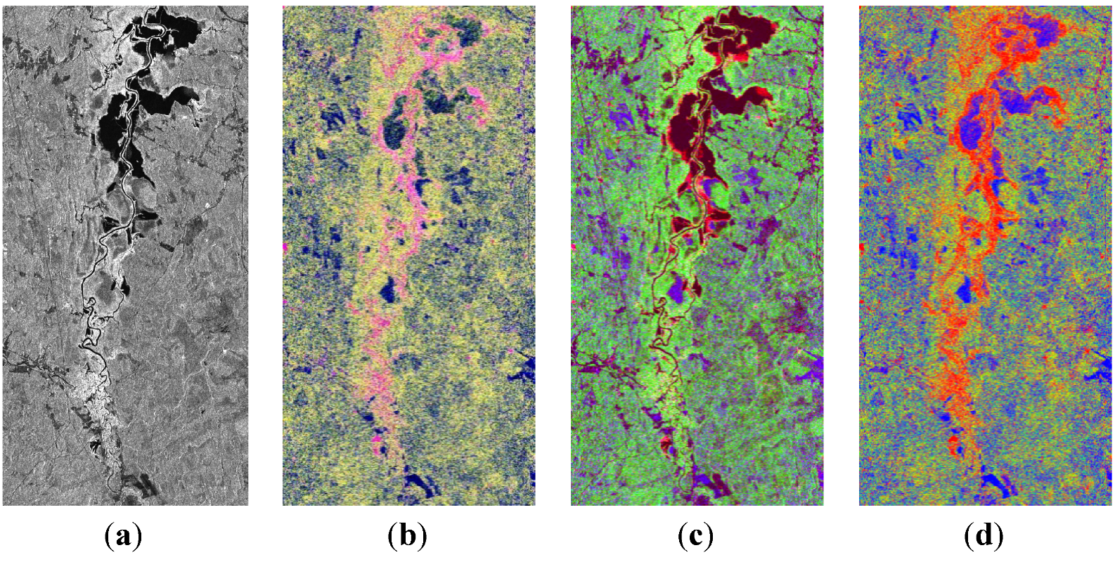The following images (Figure 2) only show one subset of the original scene in order to highlight areas of interest. The subset measures about 26 km in height and 14 km in width. Detailed explanations on the meaning of the polarimetric layers used for the quicklooks in Figure 2 are given in the following sections.

Figure 2. Quicklooks for different polarimetric decompositions of the first image dating from 27 April 2010. (a) Total intensity equal to Kennaugh K₀; (b) Cloude-Pottier RGB: Mean Alpha, Entropy, Anisotropy; (c) Freeman-Durden RGB: Double-bounce, Volume, Surface; and (d) Kennaugh RGB: −k₂, −k₁, −k₃.

Figure 2. Quicklooks for different polarimetric decompositions of the first image dating from 27 April 2010. (a) Total intensity equal to Kennaugh K₀; (b) Cloude-Pottier RGB: Mean Alpha, Entropy, Anisotropy; (c) Freeman-Durden RGB: Double-bounce, Volume, Surface; and (d) Kennaugh RGB: −k₂, −k₁, −k₃.

3.2. Polarimetric Decompositions

Studying rural landscapes where many distributed targets are present requires incoherent polarimetric decompositions, i.e., the measured polarization channels are integrated in a backscattering matrix—Coherence matrix T, Covariance Matrix, or Kennaugh Matrix K—and subsequently averaged over several neighbouring resolution cells. The incoherent averaging here is performed by interpolating the slant range image during the geocoding process. Hence, a—partially—incoherent scattering description is achieved. In general there are three approaches to decompose and/or interpret these incoherent descriptors:

(1)

Decompose the distributed target information into the contributions of deterministic targets (Cloude-Pottier);

(2)

Extract intensities of different backscatter mechanisms according to a certain scattering model (Freeman-Durden);

(3)

Appropriately scale and directly interpret the backscattering matrix elements themselves (Normalized Kennaugh elements).

The Cloude-Pottier decomposition [11] bases on the coherency matrix T which correlates the coherent Pauli vectors that consists of odd-bounce, even-bounce, and diffuse scattering elements. Because of the mathematical characteristics of the coherency matrix it can be expressed by the help of three orthogonal complex eigenvectors [combined in matrix U, see Equation (2)] that are scaled by three real positive eigenvalues λ_1,2,3, see Equation (1). Each combination of eigenvalue and eigenvector represents one coherent scattering mechanism in the incoherent descriptor whereupon the eigenvalue [Equation (1)] gives the strength of the scattering mechanism and the eigenvector [Equation (2)] defines the type of backscattering.

(1)

(2)

As the interpretation of the three scattering vectors at once is very complicated, further parameters describing the relations between the three scattering mechanisms are derived. The entropy describes the heterogeneity or the incoherency of the signal adopting low values for only one and high values for three equipollent targets. For mean values of the entropy the relationship between the second and the third eigenvalue is of interest and is defined as the anisotropy. The scattering type is indicated by the angle α which can be specified as dominant α—only for the strongest target—or as mean α—weighted average out of all three target vectors. This parameter ranges around 45° for volume scattering, decreases towards surface scattering and increases towards double-bounce. The remaining angle parameters refer to target rotation and target shape. Those will not be taken into account in this study.

The Freeman-Durden decomposition [12] exclusively treats distributed symmetric targets described by the covariance matrix C for which the scattering matrix adopts the form displayed in Equation (3): Only the co-polarized correlations (S_HHS_VV^*, S_VVS_HH^*) and the co- and cross-polarized intensities (I_HH, I_VV, I_HV) remain while all other elements are set to zero. By the help of a scattering model that defines the standardized covariance matrices for the three scattering mechanisms (C_surf, C_dbl, C_vol) their influence —equal to their intensity (I_dbl, I_vol, I_surf) —on the measured covariance matrix is estimated. The result of this decomposition thus comprises three intensity layers corresponding to surface, diplane, and volume scattering.

(3)

The Normalized Kennaugh elements [13] represent an alternative to conventional polarimetric decompositions. As any decomposition approach necessarily reduces the number of channels and thus, unavoidably the information content, this method tries to interpret the elements of the scattering matrix themselves. The Kennaugh matrix that originates from polarization optics was chosen to be the optimal representation. Its elements can be calculated from the measured polarization channels as follows [Equation (4)]:

(4)

The first element K₀ always reflects the total intensity. The others can be divided into absorption, diattenuation, and retardance elements along the directions parallel, diagonal and circular. The elements K₁, K₂, K₃ (e.g.,) define the absorption difference parallel, diagonal, and circular in relation to the coordinate system. K₄ and K₇ both belong to the parallel direction and contain the diattenuation and retardance respectively. Kennaugh elements evaluating the cross-polarized phase information are not taken into account because the phase angle differences between co-polarized and cross-polarized channels are widely stochastic over natural environments [11]. In order to guarantee a uniform value range—for display and archiving reasons—all Kennaugh elements are normalized according to Equation (5) by the total intensity or the reference intensity of 1—in the case of the total intensity itself—and subsequently brought to decibel units by the help of the inverse hyperbolic tangent function tanh⁻¹, see Equation (6).

(5)

(6)

3.3. Change Detection Method

Curvelets are a relatively new alternative image representation. Instead of interpreting an image pixel-by-pixel it is decomposed into a collection of multi-scale, multi-orientation, and multi-location ridge-like structures. These structures can be manipulated by the help of the assigned complex Curvelet coefficient in order to select distinct structures and suppress noise. Therefore, the Curvelet based change detection [11] method originally was developed for change detection in highly structured areas like urban environments [2]. Being sensitive towards elongated structures—because of the “ridges” used for decomposition—it seems to be an appropriate tool for surveying the flooded vegetation bands along rivers. Defined for the processing of image data with additive characteristics—i.e., optical images or logarithmic SAR intensities—the outputs of the polarimetric decompositions have to be scaled in order to act as input to the change detection process. Apart from that, this fully automatic change detection processor needs no further modifications.

The entropy and angle parameters of the Cloude-Pottier decomposition already possess a closed value range and a normal-like distribution, thus, no scaling is required. The layers of the Freeman-Durden decomposition are intensity values and have to be brought to logarithmic scaling before applying the change detection algorithm [11]. The Normalized Kennaugh Elements given as decibel values already show a normal-like distribution and can be introduced without further scaling. The type of change and the output units hence depend on the input data: For the Cloude-Pottier decomposition and the Normalized Kennaugh Elements the image comparison delivers additive increase and decrease respectively that are unit less (entropy and anisotropy), in degrees (α angle) or in dB (k_i). In the case of the Freeman-Durden decomposition the output images describe the logarithmic quotient—i.e., the relative increase and decrease—which can be scaled to decibel units afterwards.

4. Results

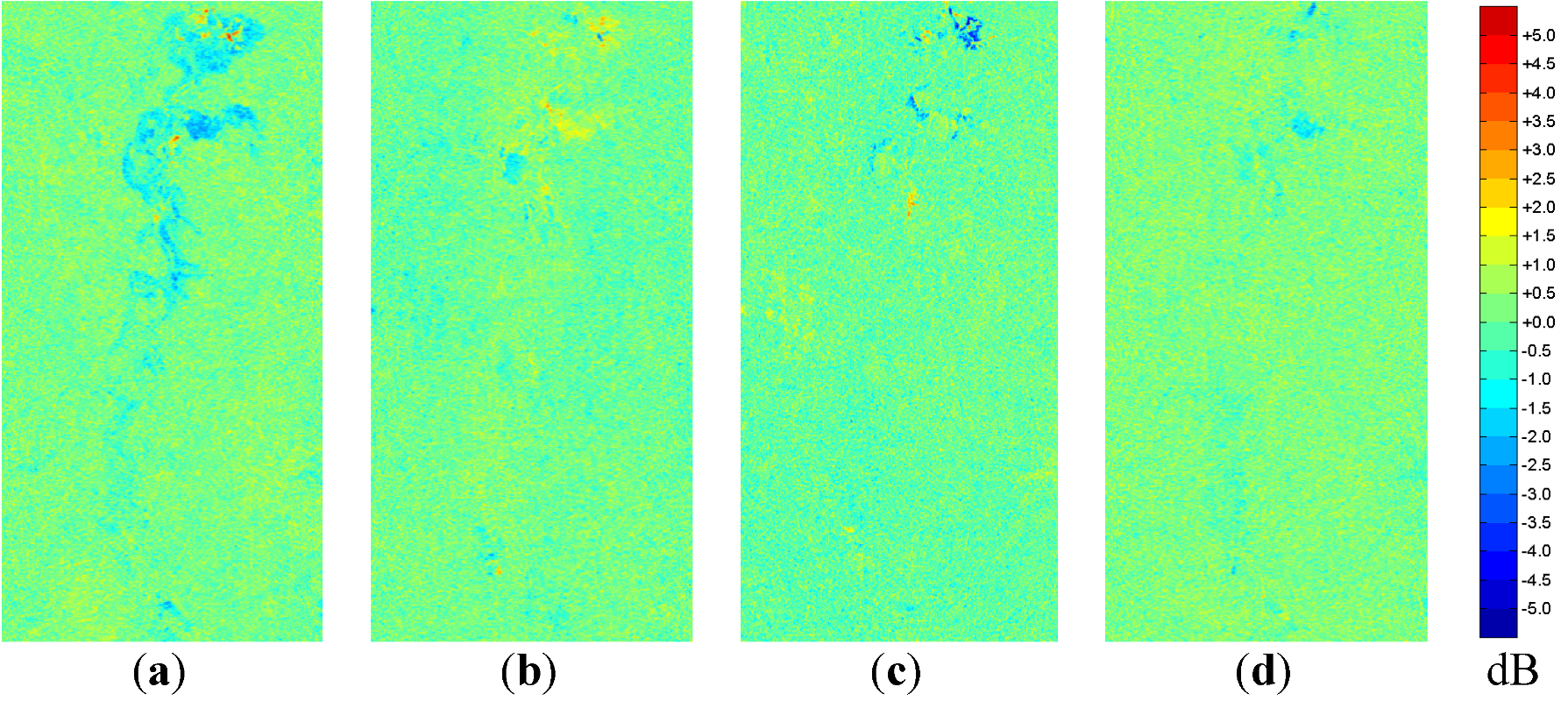
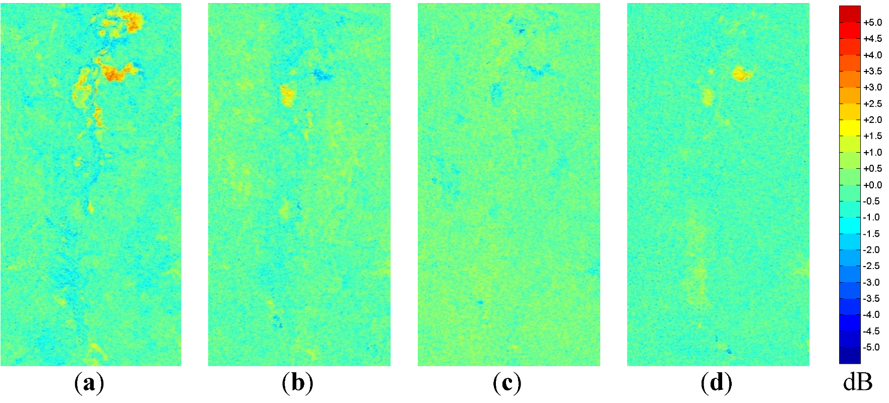
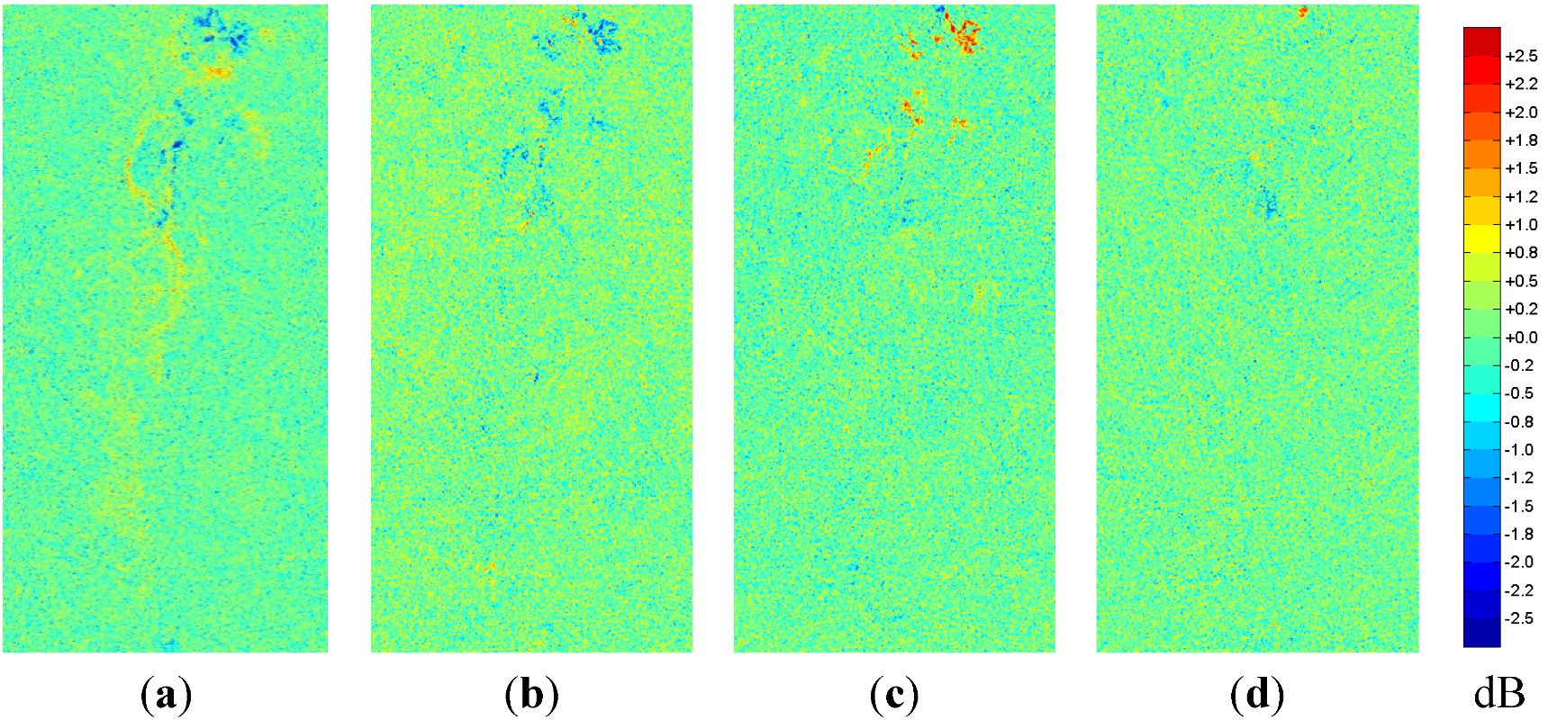
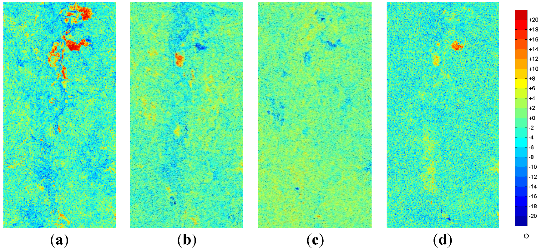
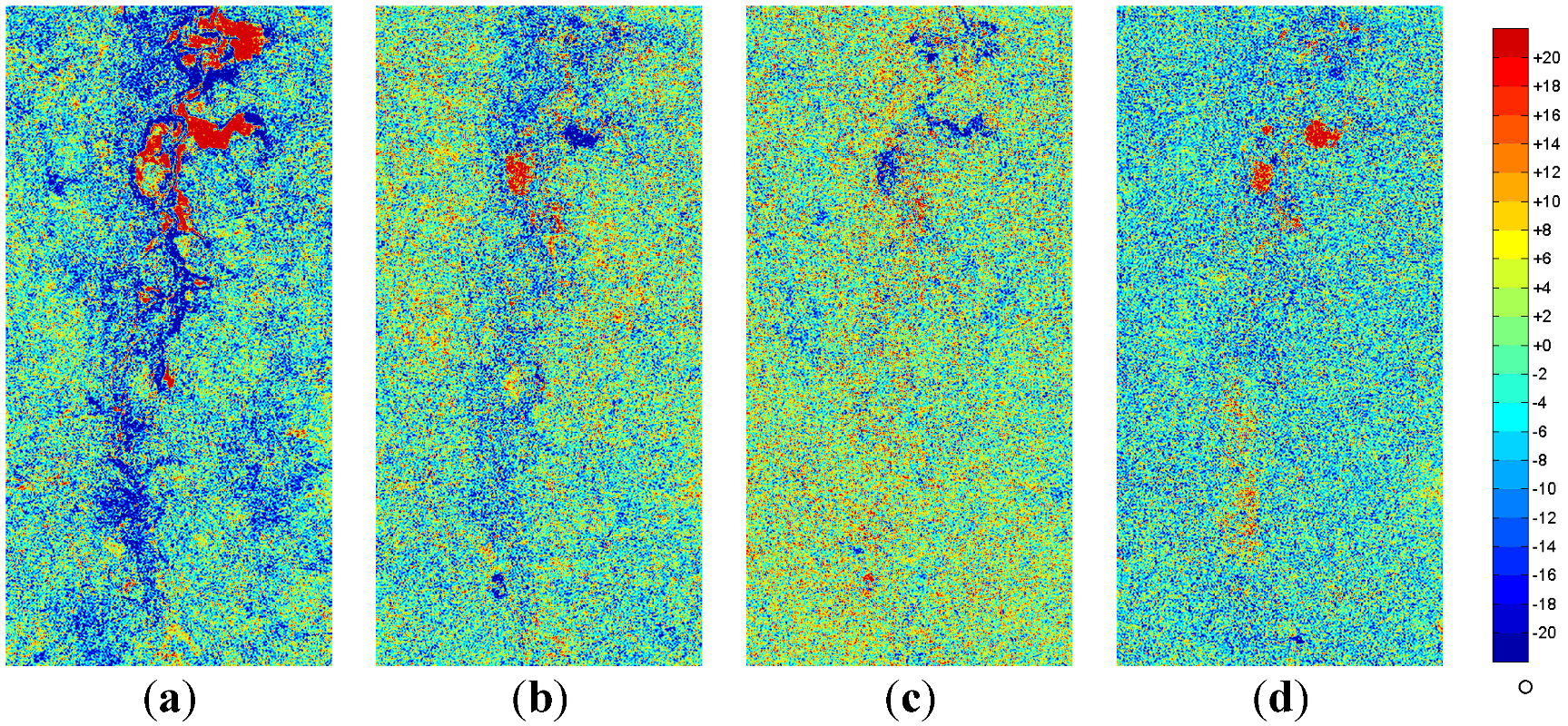
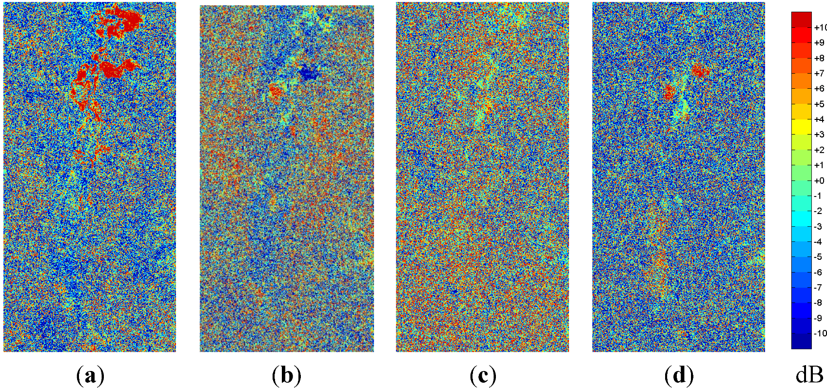
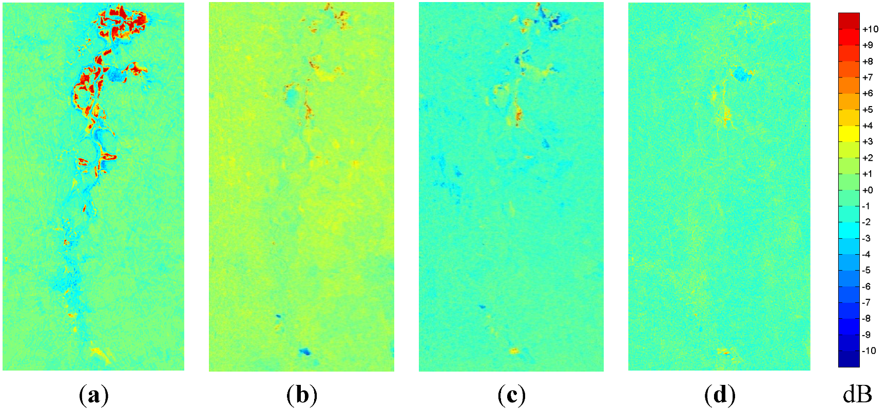
The continuous change detection results are presented in this section. Four comparison images can be calculated from neighboring images throughout the time series: Change from April to May (a), from May to June (b), from June to July (c), and from July to August (d). The color coding is uniform for all images starting with blue for strong negative changes, showing green for only minor changes and ending with red for high positive changes. The corresponding units are given in the color bar at the right side of the images. The meaning of the changes detected is explained in the following sections.

4.1. Cloude-Pottier-Decomposition

The change in entropy according to the Cloude-Pottier decomposition is displayed in Figure 3. Positive changes refer to an increase in heterogeneity, i.e., that there is a development away from one dominant target towards three equally strong backscattering mechanisms. Blue by the way indicates the converse development. The changes in anisotropy (Figure 4) show higher differences between the second and the third eigenvalue in red and the assimilation of both in blue. The α angles—representing the scattering type—can be found in Figure 5, Figure 6. For both red indicates an increase in double-bounce while blue stands for an increase in surface scattering.

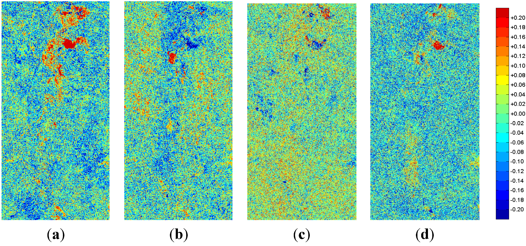
Figure 3. Cloude-Pottier entropy changes between sequent acquisitions (without unit): (a) April to May; (b) May to June; (c) June to July; and (d) July to August.

Figure 3. Cloude-Pottier entropy changes between sequent acquisitions (without unit): (a) April to May; (b) May to June; (c) June to July; and (d) July to August.

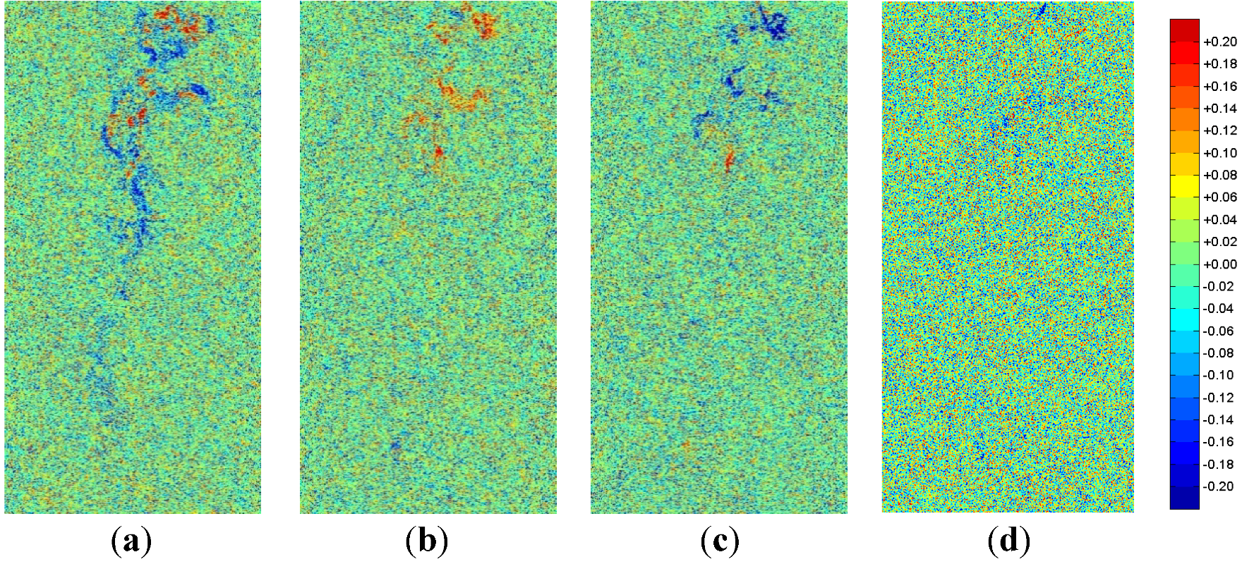
Figure 4. Cloude-Pottier anisotropy changes between sequent acquisitions (without unit): (a) April to May; (b) May to June; (c) June to July; and (d) July to August.

Figure 4. Cloude-Pottier anisotropy changes between sequent acquisitions (without unit): (a) April to May; (b) May to June; (c) June to July; and (d) July to August.

Figure 5. Cloude-Pottier mean alpha changes between sequent acquisitions in degrees: (a) April to May; (b) May to June; (c) June to July; and (d) July to August.

Figure 5. Cloude-Pottier mean alpha changes between sequent acquisitions in degrees: (a) April to May; (b) May to June; (c) June to July; and (d) July to August.

Figure 6. Cloude-Pottier dominant alpha changes between sequent acquisitions in degrees: (a) April to May; (b) May to June; (c) June to July; and (d) July to August.

Figure 6. Cloude-Pottier dominant alpha changes between sequent acquisitions in degrees: (a) April to May; (b) May to June; (c) June to July; and (d) July to August.

4.2. Freeman-Durden-Decomposition

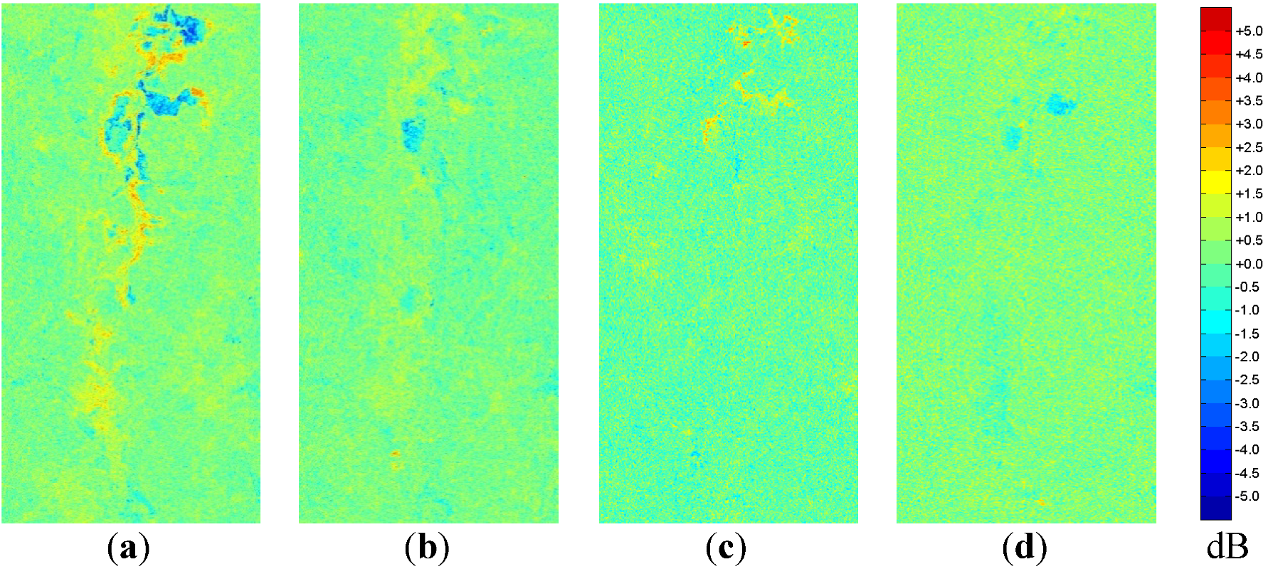
As all output layers the Freeman-Durden decomposition are intensity values the following images show the relative change in decibel for the corresponding scattering type, e.g., red symbolizes an increase in double-bounce scattering (Figure 7) and green means a reduction of the double-bounce scattering contribution. The same interpretation applies to the surface scattering in Figure 8 and the volume scattering in Figure 9.

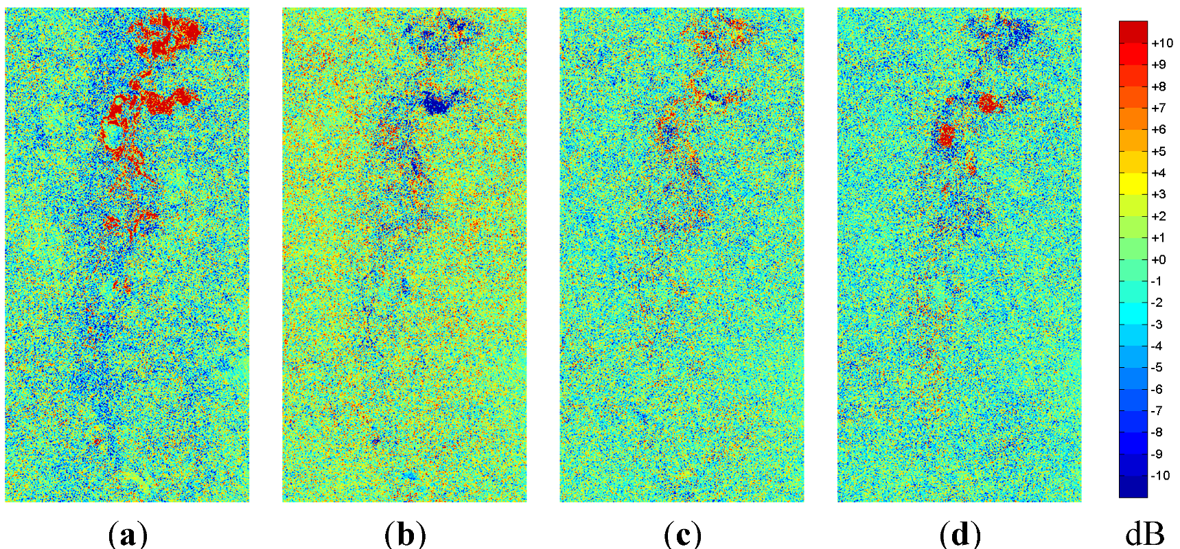
Figure 7. Change in double-bounce scattering intensity according to the Freeman-Durden decomposition between sequent acquisitions scaled to decibel values: (a) April to May; (b) May to June; (c) June to July; and (d) July to August.

Figure 7. Change in double-bounce scattering intensity according to the Freeman-Durden decomposition between sequent acquisitions scaled to decibel values: (a) April to May; (b) May to June; (c) June to July; and (d) July to August.

Figure 8. Change in surface scattering intensity according to the Freeman-Durden decomposition between sequent acquisitions scaled to decibel values: (a) April to May; (b) May to June; (c) June to July; and (d) July to August.

Figure 8. Change in surface scattering intensity according to the Freeman-Durden decomposition between sequent acquisitions scaled to decibel values: (a) April to May; (b) May to June; (c) June to July; and (d) July to August.

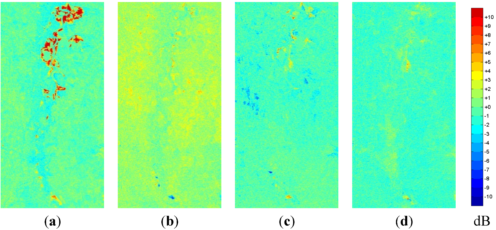
Figure 9. Change in volume scattering intensity according to the Freeman-Durden decomposition between sequent acquisitions scaled to decibel values: (a) April to May; (b) May to June; (c) June to July; and (d) July to August.

Figure 9. Change in volume scattering intensity according to the Freeman-Durden decomposition between sequent acquisitions scaled to decibel values: (a) April to May; (b) May to June; (c) June to July; and (d) July to August.

4.3. Normalized Kennaugh Elements

The change in the normalized Kennaugh elements—often called differential Kennaugh elements dk—is displayed in Figure 10, Figure 11, Figure 12, Figure 13, Figure 14, Figure 15. The change in k₀ directly reflects the change in intensity: red stands for an increasing while blue indicates a decreasing backscattering strength, see Figure 10. For the remaining elements the comparison delivers the change of the corresponding relation, i.e., a development towards a certain scattering behavior. 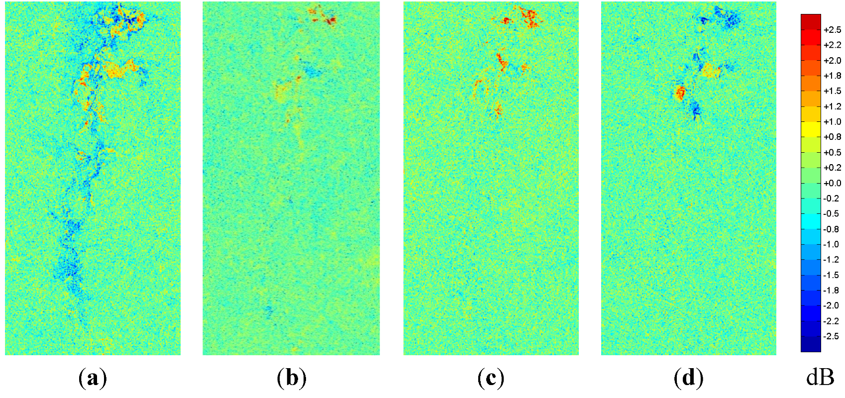For example out of the absorption elements the circular absorption k₃ in Figure 13 moves towards a positive rotation for red and towards negative—opposite direction—for blue. The parallel diattenuation exclusively containing the difference between HH and VV backscattering intensity shows red for an increase of the HH contribution and blue for a change towards VV. Thus, blue can be interpreted as an increase in the number of vertical dipoles, maybe wet culms in water. The change in parallel retardance marks the change in phase shift along the coordinate axes.

Figure 10. Change in Kennaugh Element k₀ (total intensity) between sequent acquisitions scaled in decibel: (a) April to May; (b) May to June; (c) June to July; and (d) July to August.

Figure 10. Change in Kennaugh Element k₀ (total intensity) between sequent acquisitions scaled in decibel: (a) April to May; (b) May to June; (c) June to July; and (d) July to August.

Figure 11. Change in Kennaugh Element k₁ (parallel absorption) between sequent acquisitionsscaled in decibel: (a) April to May; (b) May to June; (c) June to July; and (d) July to August.

Figure 11. Change in Kennaugh Element k₁ (parallel absorption) between sequent acquisitionsscaled in decibel: (a) April to May; (b) May to June; (c) June to July; and (d) July to August.

Figure 12. Change in Kennaugh Element k₂ (diagonal absorption) between sequent acquisitions scaled in decibel: (a) April to May; (b) May to June; (c) June to July; and (d) July to August.

Figure 12. Change in Kennaugh Element k₂ (diagonal absorption) between sequent acquisitions scaled in decibel: (a) April to May; (b) May to June; (c) June to July; and (d) July to August.

Figure 13. Change in Kennaugh Element k₃ (circular absorption) between sequent acquisitionsscaled in decibel: (a) April to May; (b) May to June; (c) June to July; and (d) July to August.

Figure 13. Change in Kennaugh Element k₃ (circular absorption) between sequent acquisitionsscaled in decibel: (a) April to May; (b) May to June; (c) June to July; and (d) July to August.

Figure 14. Change in Kennaugh Element k₄ (Parallel Diattenuation) between sequent acquisitions scaled in decibel: (a) April to May; (b) May to June; (c) June to July; and (d) July to August.

Figure 14. Change in Kennaugh Element k₄ (Parallel Diattenuation) between sequent acquisitions scaled in decibel: (a) April to May; (b) May to June; (c) June to July; and (d) July to August.

Figure 15. Change in Kennaugh Element k₇ (Parallel Retardance) in decibel: (a) April to May; (b) May to June; (c) June to July; and (d) July to August.

Figure 15. Change in Kennaugh Element k₇ (Parallel Retardance) in decibel: (a) April to May; (b) May to June; (c) June to July; and (d) July to August.

5. Discussion

The three decompositions compared in this study focus on different aspects of the polarimetric signal received. The Cloude-Pottier decomposition develops parameters to describe the relation of the three coherent targets in the resolution cell, the Freeman-Durden decomposition extracts intensities according to a pre-defined scattering model and the Normalized Kennaugh elements lend a physical meaning to the single elements of the incoherent backscattering matrix. The following section will exclusively discuss the suitability of the decompositions for this special application: wetland monitoring.

The entropy and anisotropy layers of the Cloude-Pottier decomposition (Figure 3, Figure 4) obviously are characterized by a very high noise content. Additionally, their change is not easy to interpret at all. In contrast, the α angles (Figure 5, Figure 6) can easily be referred to changes in the landscape: higher alpha means more flooded vegetation, lower alpha means less flooded vegetation, in which the dominant α angle shows more and stronger changes along the river and the mean α angle delivers much smoother results. The reason can be found in the definition of both. As the double-bounce effect always causes a very strong backscattering, it will mostly appear as the dominant backscattering mechanism in the resolution cell, i.e., in the dominant α angle. Where several equally strong targets are summed up in one resolution cell the α angle of the dominant—the strongest—one becomes somehow arbitrary. The mean alpha angle averaging the scattering type over all extracted targets deliver more robust and thus, more smooth results there. Unfortunately, because of the missing intensity layer changes concerning the open water surfaces are not visible in the change images.

The Freeman-Durden decomposition is divided in two steps: first the volume scattering component is extracted as ratio of the HV component and subsequently the remaining scattering information is classified into dominant double-bounce or dominant surface scattering in order to select the further processing steps. As this classification only delivers robust results as long as there is one really dominant target, the decision again becomes arbitrary when the scattering contributions of surface and double-bounce are approximately equal. Thus, the change detection images in Figure 7, Figure 8 appear very noisy except along the river. In contrast to that, the change in the volume component in Figure 9 is very smooth because this layer was calculated before the classification step.

In order to map the changes in flooded vegetation the change in the double-bounce layer can be used. The change in open water surfaces—i.e., a change in intensity—will produce similar changes over all three channels.

The Normalized Kennaugh elements obviously result in much smoother change images than the preceding ones though using the identical change detection algorithm. Being nothing else than linear combinations of the correlations between the measured polarization channels there is no classification process or eigenvalue decomposition that might heighten the noise content and additionally, the calculation effort is minimal. Furthermore, as the H-V coordinate system plays a key role in the definition of the Kennaugh elements, those elements including co- to cross-polarized correlations can be rejected because of their low information content over natural land cover. The change in k₀ (Figure 10) can directly be referred to the change in open water surface. Red clearly indicates the disappearance of open water surfaces i.e., falling water gauge. Amongst the absorption elements mainly the diagonal absorption k₂ shows interesting results: the yellow lines point to an increase in surface scattering, i.e., formerly flooded land now fallen dry while the deep blue areas indicate an increase in double-bounce i.e., more flooded vegetation. The circular absorption k₃ (Figure 13) in parts looks like the inversion of the element k₂ in Figure 12. The definitions in Equation 4 show this correlation. Thus, in future it will be enough to use one of both. The change in parallel diattenutation—the relation of HH to VV intensity—also reveals clear structures, see Figure 14. Blue might be interpreted as an increase of small vertical dipoles, e.g., wet culms causing a higher reflectance in VV while red stands for an increase of horizontal dipoles. The parallel retardance k₇ (Figure 15)—though containing some structures—is more affected by noise and not easy to interpret as change in the landscape. In summary, the change in open water surface can easily be detected by comparing k₀ and the change in flooded vegetation is indicated by k₂ and k₄ which even might allow a more detailed characterization of the flooding situation.

6. Conclusions

Three decomposition techniques for polarimetric SAR data have been tested for suitability for wetland monitoring with focus on open water and flooded vegetation. The time series of RADARSAT‑2 FineQuad data have been evaluated by the Curvelet-based change detection approach that automatically calculates and enhances the difference image in the Curvelet coefficient domain. Thus, the quality of the change detection results directly reflects the quality of the decomposition.

Amongst the three decompositions the Normalized Kennaugh elements turn out to be the most appropriate description for polarimetric data of wetlands because some of the layers can directly be attached to land cover types and land cover changes respectively. Thus, the number of layers needed can be reduced. On the other hand it delivers the smoothest and consequently the most distinct results. The Kennaugh elements recommended for wetland monitoring are k₀, k₂ and k₄.

As those elements predominantly hold information from the co-polarized layers—i.e., HH and VV—it is feasible to replace the quad-polarized image acquisition by a dual-co-polarized imaging mode enabling higher geometric resolution and larger coverage at the same time. Therefore, future studies will combine multi-polarized data of different sensors—e.g., RADARSAT-2 and TerraSAR-X—in order to highlight synergistic effects in the context of wetland monitoring and other fields of application.