Groundwater Risk Assessment Model (GRAM): Groundwater Risk Assessment Model for Wellfield Protection

Abstract

A groundwater risk assessment was carried out for 30 potable water supply systems under a framework of protecting drinking water quality across South Australia. A semi-quantitative Groundwater Risk Assessment Model (GRAM) was developed based on a “multi-barrier” approach using likelihood of release, contaminant pathway and consequence equation. Groundwater vulnerability and well integrity have been incorporated to the pathway component of the risk equation. The land use of the study basins varies from protected water reserves to heavily stocked grazing lands. Based on the risk assessment, 15 systems were considered as low risk, four as medium and 11 systems as at high risk. The GRAM risk levels were comparable with indicator bacteria—total coliform—detection. Most high risk systems were the result of poor well construction and casing corrosion rather than the land use. We carried out risk management actions, including changes to well designs and well operational practices, design to increase time of residence and setting the production zone below identified low permeable zones to provide additional barriers to contaminants. The highlight of the risk management element is the well integrity testing using down hole geophysical methods and camera views of the casing condition.

1. Introduction

A drinking water system is often described as an integrated chain of supply from source to tap or catchment to consumer [1,2]. When groundwater is the source for public water supply, understanding the impacts of land use and aquifer vulnerability are fundamental to groundwater protection. The risks to groundwater are two-fold—adverse land use and over extraction—thus requiring a dual nature of protection [3,4,5]. Therefore, it is important to identify which aquifer systems are at high risk in order to adopt appropriate risk management options.

Groundwater vulnerability assessment, such as the DRASTIC index [6] or the GODS index [7] have been used as early attempts of assessing risk to groundwater [8,9,10]. Index models are based on rating scores and key attributes such as depth to water, annual recharge, aquifer media, soil media, topography, vadose zone impact, and hydraulic conductivity [6]. These factors are weighted according to their relative importance in determining the ability of a pollutant to reach the aquifer and mapping areas of high groundwater vulnerability [11,12,13]. The common feature of the index approach is the additive utility assumption [14] such as in multi-criteria decision analysis (MCDA). Whilst the MCDA approach is commonly used because of its simplicity, disadvantages of this method include attributes with high value that compensate those with low values and vice versa [14].

Several process based approaches exist for assessing whether a contaminated site or surface applied chemicals constitutes a risk to groundwater [15,16,17,18,19]. Such an approach requires modeling of pollutant transport and fate. Similarly, statistical methods based on the concepts of uncertainty have been developed [20,21,22]. Both methods require an extensive data base, including monitoring and actual measurements of contaminant concentrations to calibrate and validate the models. Therefore, process based risk assessments are often subject to data limitations and significant uncertainties [23]. Uncertainties may arise from poor conceptual understanding, overly simplified assumptions about subsurface fate and transport or lack of soil and aquifer parameters. The conceptual uncertainties have been recognized as the most significant sources of error [24,25].

Such approaches can be useful for detailed risk assessment, but are of limited value to groundwater managers who need to achieve proactive and timely groundwater protection across extensive groundwater basins. For this purpose, risk screening models such as the Pattle Delamore Partners model [26], which is a modification of the Canadian Council of the Ministers of the Environment (CCME) [27] risk screening model are more useful. The assessment process of the Pattle Delamore Partners model is based upon the hazard-pathway-receptor risk equation. Although the model is fundamentally qualitative, numerical scores are assigned to various risk parameters, hence it is semi-quantitative. The ranking system is multiplicative rather than additive.

Development of a microbial contamination susceptibility model for private groundwater sources has been carried out by assessing the presence of thermotolerant coliform (TTC) in groundwater [28]. Risk analysis in the study [28] shows that source type, groundwater vulnerability, subsoil type, and set back distance from septic tanks are all important factors for the presence of TTC. However, risk assessment tools and risk management actions must be proactive rather than being a reactive response to the detection of coliform bacteria. In the first instance, risk has to be assessed using external parameters such as using the likelihood of release of risk agent, and pathway to the receptor. This is in support of new wells being drilled and new wellfields being developed to support water supply. Risk assessment tools and risk management actions also have a role in the proactive design of an adequately (water quality) sampling regime, and can be set up to include new information such as the detection of coliform bacteria and increasing salinity, once they become available.

In this paper, we present a semi-quantitative Groundwater Risk Assessment Model (GRAM) based on a multi-barrier approach to wellfield protection. The unique feature of GRAM is incorporation of groundwater vulnerability and well integrity into the risk equation. We applied the model to 30 potable water supply wellfields across South Australia, then implemented risk management actions to the identified high risk wellfields to secure the long-term quality of the groundwater source.

2. Methods

The GRAM is based on the premise that quantitative risk (R) can be expressed as a function of the complete set of triplets [29]:

R = {< s_i, l_i, x_i >}_c

(1)

• (s_i) = What can go wrong (what can happen or identification of hazard)?
• (l_i) = How likely is that to happen (what is its frequency/probability or likelihood)?
• (x_i) = If it does happen, what are the consequences (what is the damage)?

The index i specifies that more than one scenario may be of interest, curly brackets indicate a set of answers and index c indicates possible scenarios of interest that are considered [30]. The multiplicative semi-quantitative risk assessment approach is widely used in a variety of risk assessment models [31,32,33,34,35]. The GRAM is based on three distinct criteria: likelihood of release, exposure pathway to receptor and consequence. The ranking system is designed to avoid ultra-low scores which will result in removal of risk associated with a site. 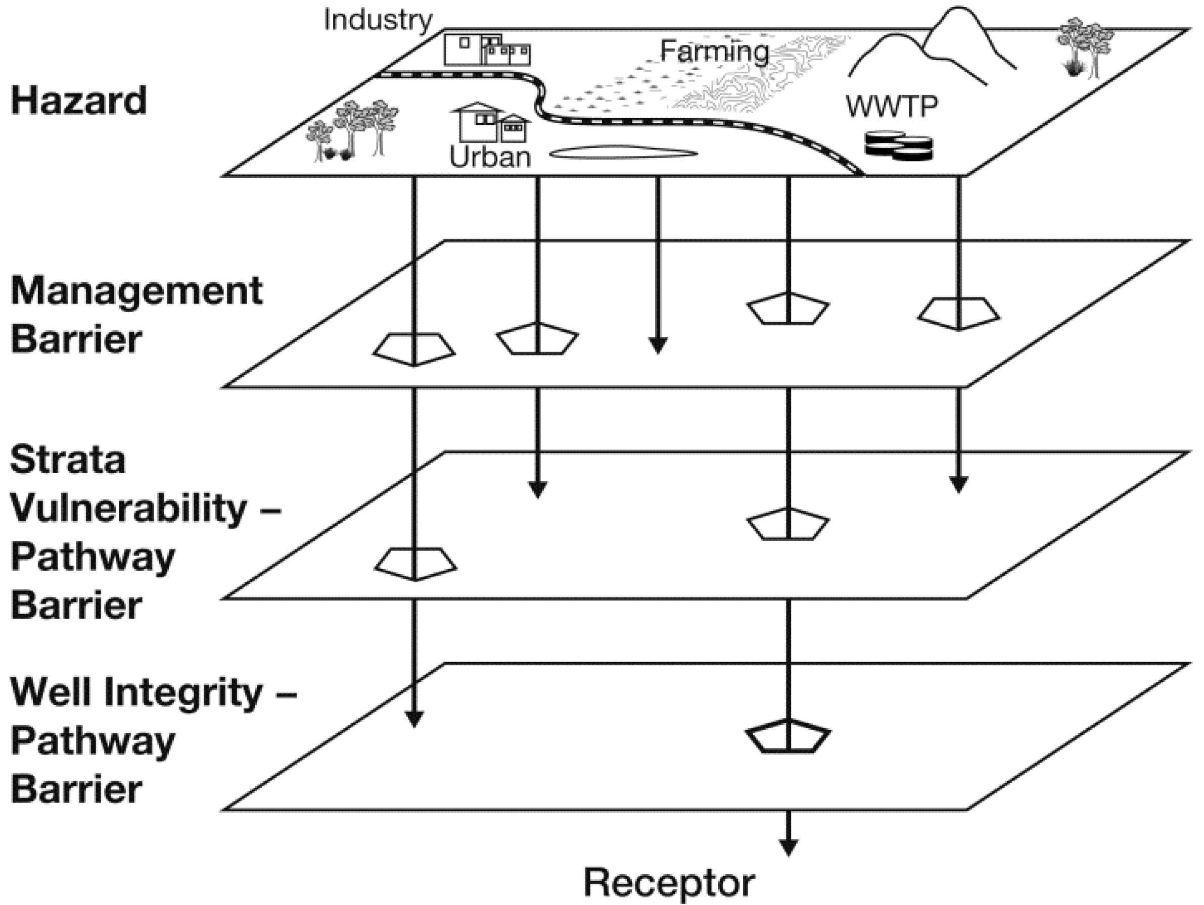The system is consistent with the Australian Drinking Water Guidelines’ (ADWG) [2] generic risk matrix. The model incorporates as many physical parameters as possible in order to reduce parameter uncertainty. The multi-barrier approach is followed based on implementation of multiple barriers throughout from hazard to receptor (Figure 1).

Figure 1. Conceptual model of the groundwater risk assessment model (GRAM).

Figure 1. Conceptual model of the groundwater risk assessment model (GRAM).

2.1. Likelihood of Release (Management Barrier)

Proactive catchment management is considered to be the first barrier and the likelihood of release of contaminants depends on how best the hazards are managed in the supply catchments. The assessment process starts by describing the potential of hazards being released into the environment. This is divided into four distinct categories, each having five levels. These levels are assigned scores based on both quantitative and qualitative criteria including informed judgments. The range of scores is derived from the Prattle Dellamore model [26] and reflects the importance and contribution to the likelihood of contaminant release, which are given in brackets in Table 1. The four categories are:

• Quantity: Release due to nature of the source, amount, type and occurrence;
• Attenuation: Contaminant characteristics, attenuation and degradation capacity;
• Control measures: Best management practices (BMP), regulations and guidelines;
• Mitigation measures: Emergency plans and effective monitoring.
• The likelihood of release is the multiplication of the above four distinct categories.

Likelihood of Release = Quantity × Attenuation × Control Measures × Mitigation Measures

(2)

Table 1. Scores for release categories.

Release Category	Category Levels
	Level 1	Level 2	Level 3	Level 4	Level 5
Quantity	consistently low quantity (0.4)	occasionally high quantity (0.5)	more frequently high quantity or continual low quantity (0.65)	frequently high quantity (0.8)	consistently high quantity (1)
Attenuation	very high (0.75)	high (0.8)	moderate (0.85)	low (0.95)	negligible (1)
Control measures	well developed and in place (0.4)	in place but not fully compliance with BMP (0.5)	moderately developed programs in place (0.65)	poorly developed programs in place (0.8)	None in place (1)
Mitigation measures	well developed and in place (0.75)	in place but not fully compliance (0.8)	moderately developed programs in place (0.85)	poorly developed programs in place (0.95)	None in place (1)

Table 1. Scores for release categories.

Release Category	Category Levels
	Level 1	Level 2	Level 3	Level 4	Level 5
Quantity	consistently low quantity (0.4)	occasionally high quantity (0.5)	more frequently high quantity or continual low quantity (0.65)	frequently high quantity (0.8)	consistently high quantity (1)
Attenuation	very high (0.75)	high (0.8)	moderate (0.85)	low (0.95)	negligible (1)
Control measures	well developed and in place (0.4)	in place but not fully compliance with BMP (0.5)	moderately developed programs in place (0.65)	poorly developed programs in place (0.8)	None in place (1)
Mitigation measures	well developed and in place (0.75)	in place but not fully compliance (0.8)	moderately developed programs in place (0.85)	poorly developed programs in place (0.95)	None in place (1)

Many of the above categories can be accessed through field survey and monitoring, but some may require experience and expert judgments. The South Australian Environment Protection Authority (SAEPA) and United States Environmental Protection Agency (USEPA) guidelines were used in assessing BMPs. In some cases, detailed groundwater flow and capture zone modelling were used, and hence, assessing the likelihood of a contaminant release from the source provides a crucial step in risk assessment. Consistent with likelihood estimates of risk assessment models [4,32,34,35], the likelihood of release was divided into five levels which are given in Table 2.

Table 2. Levels of likelihood of release.

Level	Score	Likelihood of release
1	0.1	Rare
2	0.2	Unlikely
3	0.3	Possible
4	0.6	Likely
5	1	Highly Likely

Table 2. Levels of likelihood of release.

Level	Score	Likelihood of release
1	0.1	Rare
2	0.2	Unlikely
3	0.3	Possible
4	0.6	Likely
5	1	Highly Likely

2.2. Exposure Pathway (Strata Vulnerability and Well Integrity Barrier)

The pathway component describes the likelihood of contact with, or transport to, a receptor. In this case, the receptor is considered to be a water supply well or the aquifer depending on the objectives of the risk assessment. This indicates the physical characteristics of the aquifer and its susceptibility to land use. For exposure to occur, a source of contamination or contaminated media must exist and transport from the source to a point where exposure could occur. This concept is referred to as an exposure pathway.

Two basic factors are considered to determine aquifer pollution vulnerability [7,9]:

• the level of hydraulic inaccessibility of the saturated zone of the aquifer or production zone of the water supply well;
• the contaminant attenuation capacity of the strata overlying the saturated aquifer or production zone of the water supply well.

Based on such considerations, the GODS vulnerability index [7] was used for the strata vulnerability component of the pathway barrier, which is given in Table 3.

Table 3. Aquifer vulnerability index.

Vulnerability Level	Score
Negligible	>0–0.1
Low	>0.1–0.3
Moderate	>0.3–0.5
High	>0.5–0.7
Extreme	>0.7–1.0

Table 3. Aquifer vulnerability index.

Vulnerability Level	Score
Negligible	>0–0.1
Low	>0.1–0.3
Moderate	>0.3–0.5
High	>0.5–0.7
Extreme	>0.7–1.0

Since risk assessment involves the consideration of all potential exposure pathways, well integrity (the degree to which the well is properly designed and constructed to achieve protection objectives) is considered as an important contaminant pathway. The well integrity testing using downhole geophysical methods includes gamma, neutron, caliper, density logs, casing collar locator and downhole camera view of the casing. These geophysical logs can confirm well casing construction and identify any irregularities such as reduction in casing size, casing corrosion, lamination, and low density anomalies. Downhole camera view can provide evidence of casing condition (corrosion, cracks and clogged screens), whilst the pan and tilt camera allows a detailed inspection of any area of the well casing. This ensures provision of adequate protection of the well collar, casing and sealing of the annular space against physical damage and seepage of contaminants. In this case, vulnerability levels (Table 3) were assigned based on the level of well integrity: properly maintained well integrity (Negligible), suspect of leaky casing (Moderate), corroded steel casing with no annulus sealing (High) and open dug wells and trenches (Extreme). In addition, when the water production zone of the aquifer is overlain by impermeable barriers such as stiff clay layers within an unconfined aquifer, it is considered equivalent to hydraulic confinement; hence, the vulnerability level is adjusted to Low or Negligible.

2.3. Consequence Assessment

The consequence is the outcome of an event expressed qualitatively or quantitatively being a loss, injury, disadvantage or gain [7]. There may be a range of possible outcomes associated with an event. The consequence assessment consists of describing the relationship between specified exposures to a risk agent and the consequences of those exposures. Consequence assessments typically include specifying the impact on health in the human and animal populations sustained under given exposure scenarios. In other words, the consequence assessment is the process of developing a description of the relationship between the specified exposures to a risk agent and the health and other consequences to humans and animals exposed. This may be estimated by multiplying hazard quantity by toxicity or hazard ratings [5]. In this study, the consequence score of severity is adopted from the Environment, Health and Safety manual of the University of Melbourne [33] for consequence levels, as outlined in Table 4.

Table 4. Consequence scores.

Level	Consequence	Score	Health Impact Indicator
1	Insignificant	1	An event resulting in non-detected impacts and short term isolated aesthetic impact.
2	Minor	2.5	An event resulting in non-detected impacts and short/medium term aesthetic impact requiring remedial action.
3	Moderate	5	An event resulting in public health impact causing short/medium minor illness or long-term aesthetic impact to a large population.
4	Major	10	An event resulting in public health impact causing medium/long-term severe illness resulting in medical treatment to a large population.
5	Catastrophic	20	An event resulting in public health impact causing severe illness resulting in permanent health effects to a wide population.

Table 4. Consequence scores.

Level	Consequence	Score	Health Impact Indicator
1	Insignificant	1	An event resulting in non-detected impacts and short term isolated aesthetic impact.
2	Minor	2.5	An event resulting in non-detected impacts and short/medium term aesthetic impact requiring remedial action.
3	Moderate	5	An event resulting in public health impact causing short/medium minor illness or long-term aesthetic impact to a large population.
4	Major	10	An event resulting in public health impact causing medium/long-term severe illness resulting in medical treatment to a large population.
5	Catastrophic	20	An event resulting in public health impact causing severe illness resulting in permanent health effects to a wide population.

Likelihood (or likelihood of contamination) is any unplanned event resulting in consequences and is expressed as a qualitative or quantitative description of probability or frequency. The likelihood assessment consists of describing the: (a) potential of a risk agent release from the source; and (b) existence of a pathway (the route a contaminant may follow) from hazard to the receptor. The likelihood (or likelihood of detection) is estimated using Equation (3) and residual risk by Equation (4).

Likelihood (or Likelihood of detection) = Likelihood of Release × Exposure Pathway

(3)

Residual Risk = Likelihood × Consequence

(4)

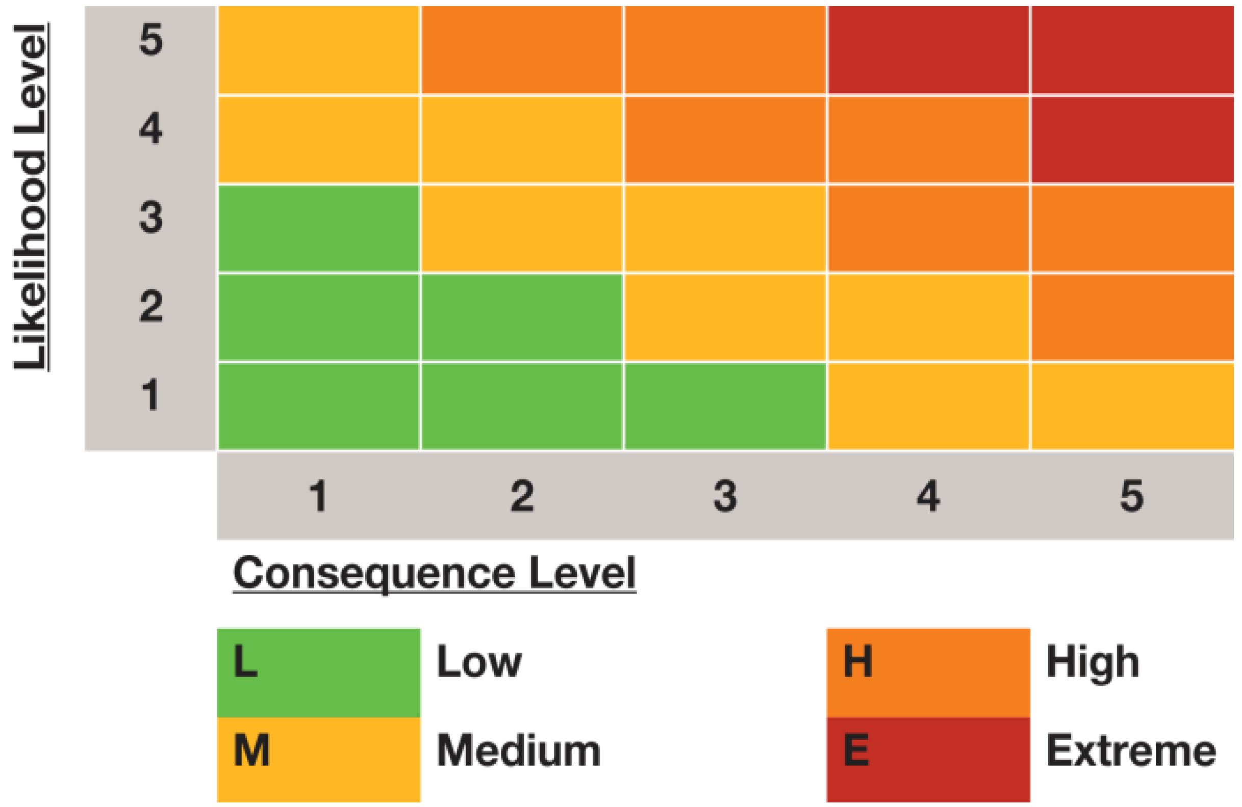
A systematic use of available information to determine how often specified events may occur and the magnitudes of their consequences is called residual risk analysis and assessment. The residual risk assessment integrates the results from release assessment, exposure assessment, and consequence assessment to produce quantitative measures of residual risk. Thereafter, the risk classes were categorised into Extreme (>10), High (2.5–10), Moderate (0.6–2.5<) and Low (0.6<) levels, in accordance with ADWG [2] and the generic risk matrix given in Figure 2.

Figure 2. Generic risk matrix.

Figure 2. Generic risk matrix.

3. Study of Groundwater Systems

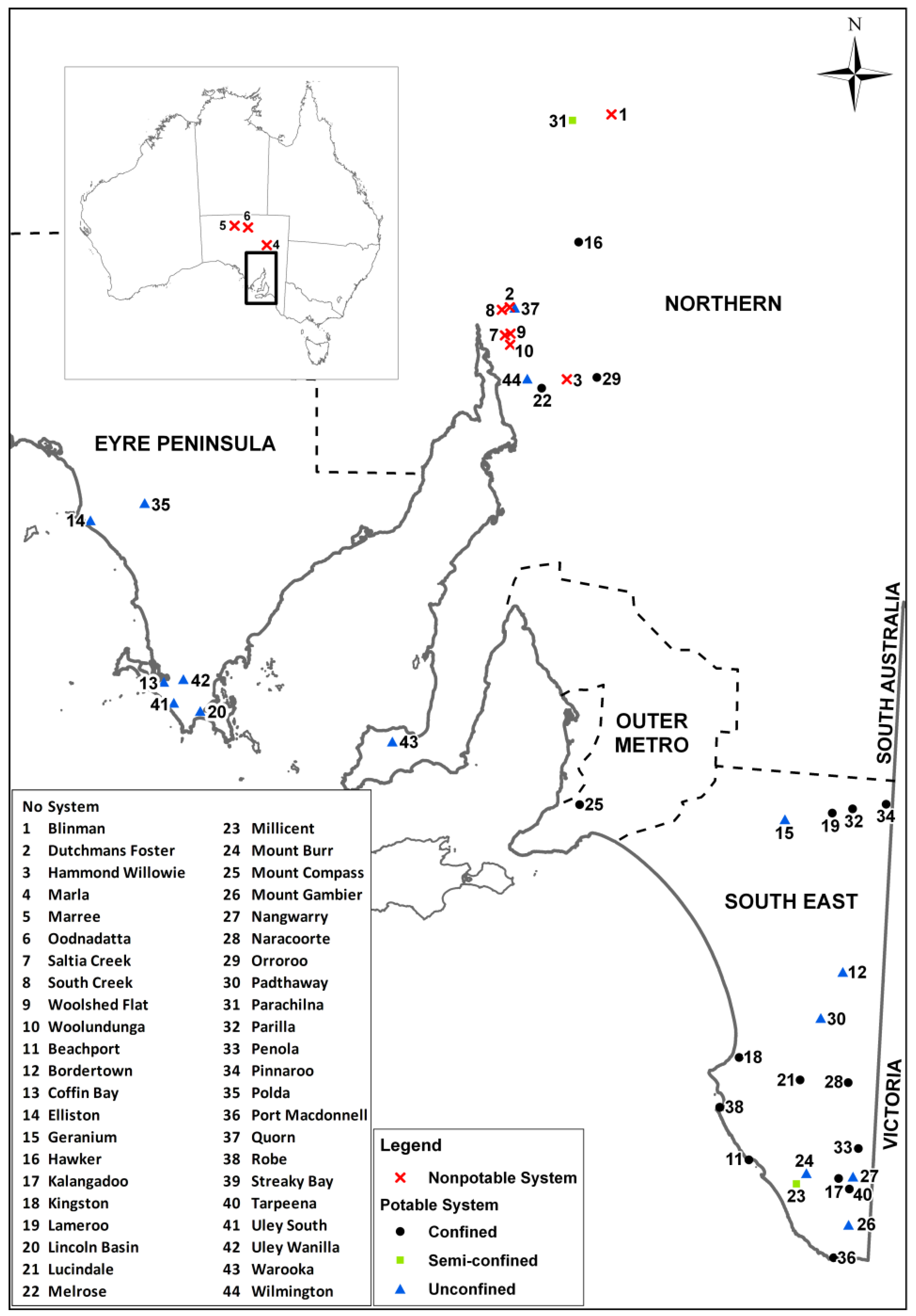
The model was tested on 30 potable town water supply systems spread across South Australia (Figure 3) that rely on groundwater as the primary domestic water supply [36] requiring protection. A risk based groundwater protection [5,37,38] was adopted and risk analysis was performed consistently across all systems in four regions.

Eyre region: The region is characterized as a temperate climate with warm to hot, dry summers and mild wet winters. Average annual rainfall and pan evaporation varies from 550 mm to 1500 mm at Port Lincoln and 375 mm to 2200 mm at Streaky Bay. The land use is predominantly broad acre cropping in winter months, and sheep grazing in summer. Low salinity groundwater occurs in the areas known as fresh water lenses, in the saturated limestone surrounded by either dry limestone or brackish water zones. Soils in the region are characterized as shallow, calcareous and overlaying calcrete or limestone. Groundwater systems in Uley South, Uley Wanilla, Coffin Bay and Robinson lens are in the South Australian Water Corporation water reserves and Lincoln basin is in a National Park.

Northern Region: The most southern water supply system in the Northern region is the Para Wurlie basin, which supplies potable water to the township of Warooka. The Para Wurlie groundwater basin is a calcareous limestone aquifer located approximately 20 km west of Warooka. The climate in the area is typically characterized by hot dry summers and wet winters, with the highest rainfall occurring between May through September. The average annual rainfall is 447 mm and average annual pan evaporation is 1400 mm. The far north of the Northern region is in arid lands and bounded by the Simpson Desert. The most northern water supply system is Marla, which receives highly variable annual rainfall of about 200 mm per year and evaporation exceeding 3300 mm per year. Except Para Wurlie basin, much of the groundwater systems extract from fractured rock aquifers or the deep confined aquifer in the Great Artesian Basin.

Figure 3. Groundwater supply systems.

Figure 3. Groundwater supply systems.

Outer Metro Region: The climate near Mount Compass is characterised by hot, dry summers and cool, wet winters. Mount Compass receives relatively high rainfall, averaging 840 mm per year. Most of the rainfall occurs in winter and early spring. The Mount Compass region has been extensively developed including irrigated horticulture (mainly berries, vegetables and olives), cattle grazing, some industry and mining. The township consists of semi-rural and residential areas. Two semi-confined water supply wells are located in a road reserve near the town.

South East Region: The climate of the South East region is characterised by cool, wet winters and hot, dry summers. Average annual rainfall varies considerably within the region, from approximately 750 mm in the south near Mount Gambier, to 250 mm in the north of the region around Pinnaroo. Potential annual evapotranspiration increases from ~1400 mm in the south to ~1800 mm in the north The dominant land use is dryland cropping and livestock grazing. There is some irrigated cropping, which includes pasture for dairy, wine grapes, lucerne, potatoes and cereals. Commercial forestry forms a significant industry in the southern part of the South East region, with both softwood and hardwood plantations. Except in Kingston SE, Millicent and Bordertown, all water supply wellfields are located within townships.

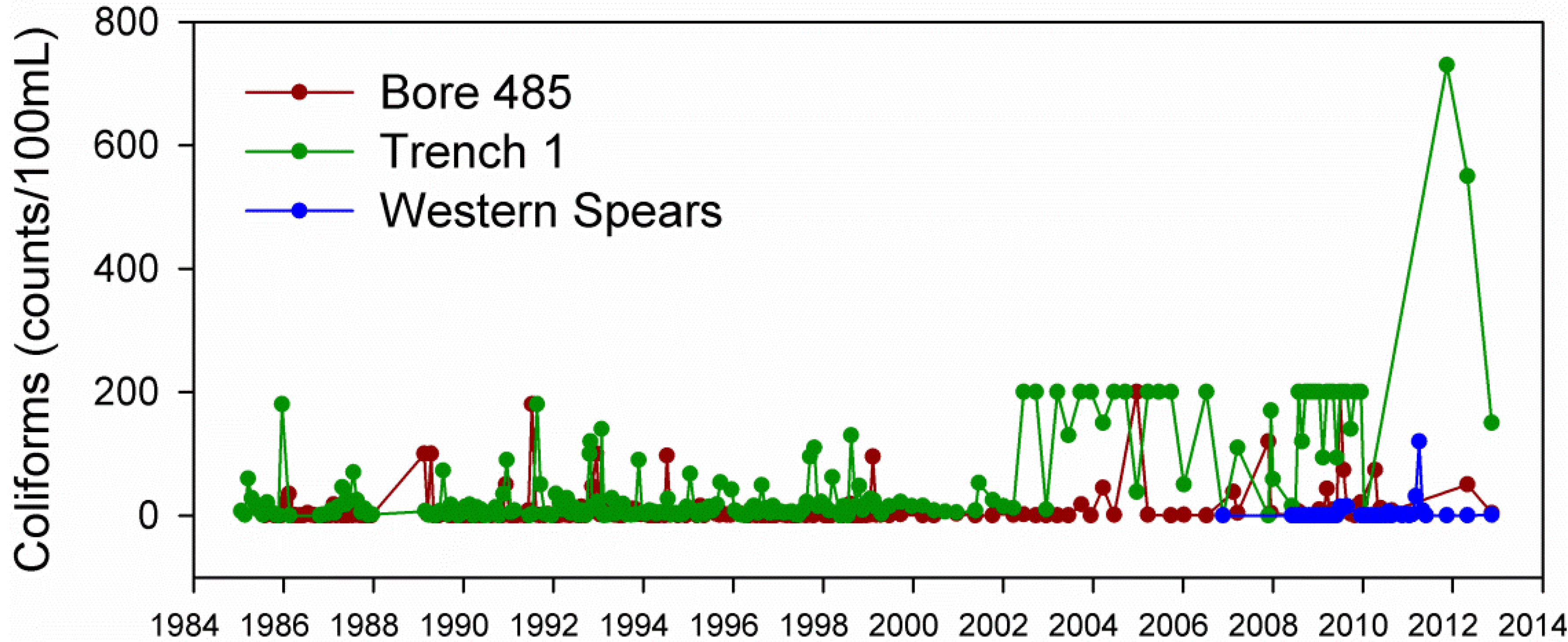
4. Results and Discussion

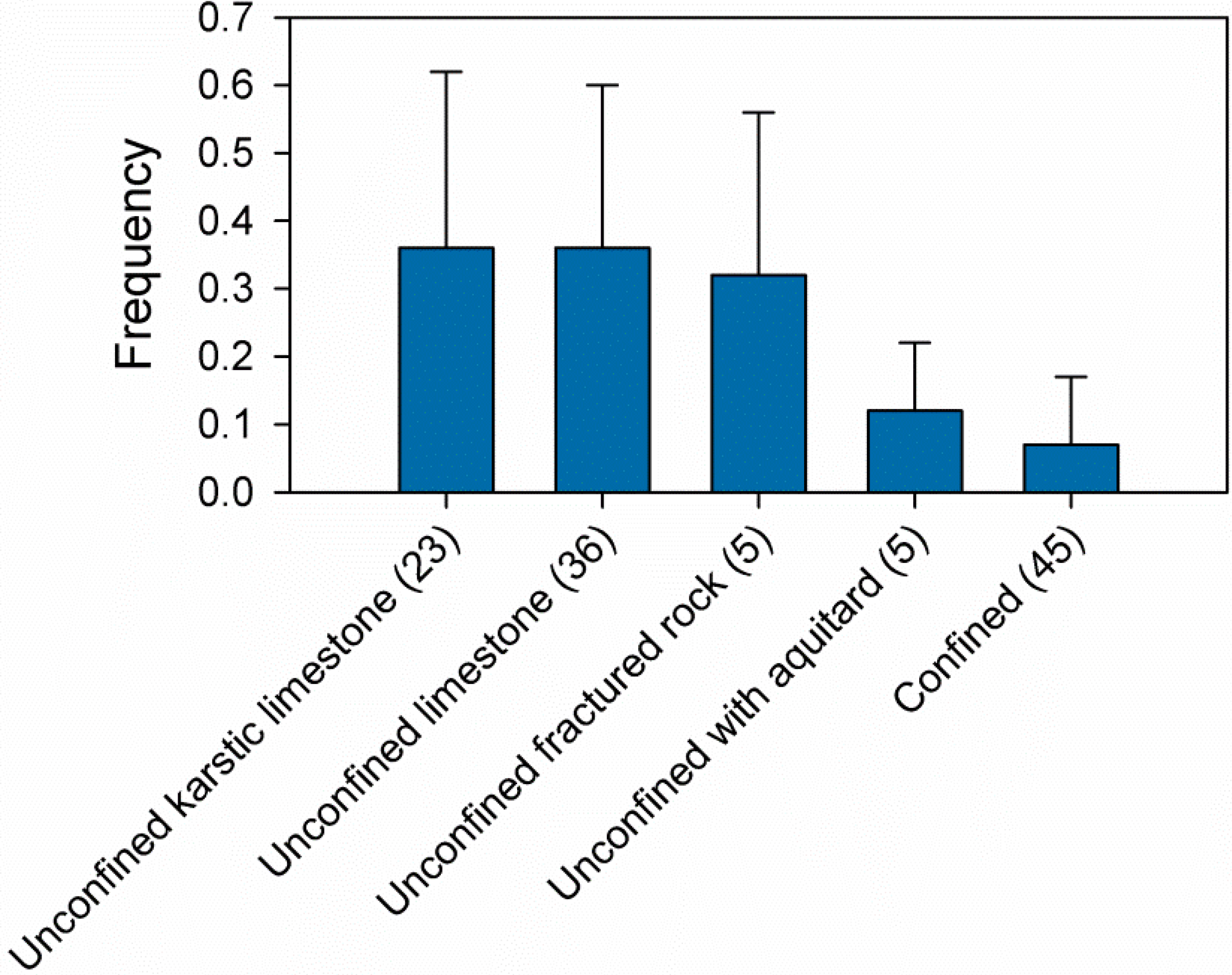
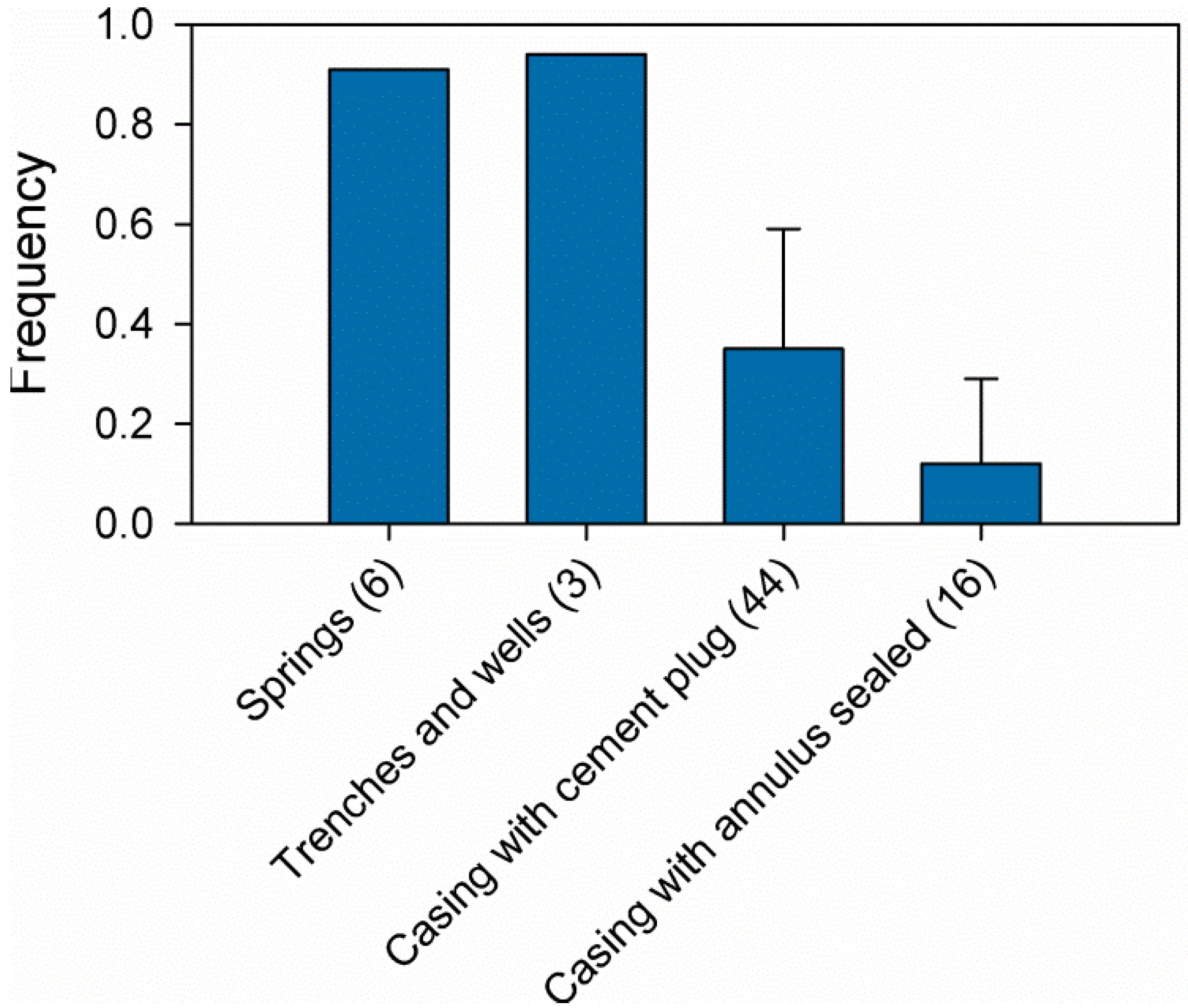
Potential sources of bacterial pollution in a catchment are many. The most prevalent and common is coliform bacteria which originate as organisms in soil or vegetation and in the intestinal tract of warm-blooded animals [39]. The bacteria could enter groundwater and water supply wells through many interacting variables related to land use, soil types, depth to water, types of geological strata and the method of well construction. Similarly, presence of nitrate in groundwater may indicate groundwater pollution, originating from land surface, particularly in rural catchments. In the absence of other significant pollutants, thus the presence of coliforms and nitrate in groundwater indicates connectivity between the ground surface and sampling zone of the aquifer, which may also facilitate the transfer of pathogens and other pollutants.

4.1. Detection of Coliform Bacteria

The survival of coliform bacteria in soil depends on the soil characteristics and warm, moist conditions for maximum survival [39]. In well aerated sandy soils, bacterial survival may be low, but if the depth to groundwater is small and the water flow rate is fast, bacterial contamination of the groundwater may be high [39]. Thus, shallow karstic aquifers and water sources that have direct contact with moist soils such as dug wells and trenches are prone to high bacterial contamination.

The number of wells available for each well construction category varied from 5 to 45, and from 3 to 44 in relation to geological strata. Where few wells are available (in some categories) rigorous statistical analysis proved difficult. Despite this, the frequency of coliform detection are clearly influenced by aquifer type, soil and geological strata (Figure 4) and well construction (Figure 5). An insufficient number of wells available in each category for assessing the likelihood of contaminant release precludes any analysis, particularly in relation to land use changes.

Figure 4. Frequency of coliform detection in relation to aquifer type and geological strata. Sample size is given in brackets.

Figure 4. Frequency of coliform detection in relation to aquifer type and geological strata. Sample size is given in brackets.

Figure 5. Frequency of coliform detection in relation to well construction. Sample size is given in brackets.

Figure 5. Frequency of coliform detection in relation to well construction. Sample size is given in brackets.

Frequent detection of coliforms with an occasional appearance of E. coli (Escherichia coli) is observed in most of the unconfined water supply wells. Historical well construction practices used steel casing with a cement plug at the casing shoe and the surface. The well annulus (annular space between the casing and the aquifer) had not been pressure cemented, and hence, provided a pathway for contaminants to move into groundwater. In Figure 6 and Figure 7, coliform and E. coli detection per 100 mL for the period of 1985–2013 is given for Robinson Lens, which is the water supply aquifer for the township of Streaky Bay. The land is a water reserve and fenced off from grazing animals, but kangaroos and rabbits are common in the reserve. Data is presented for a water supply trench (Trench 1: 25 m × 3 m × 5m), a 250 mm diameter water supply well (Bore 485) and the western wellfield comprising six 150 mm diameter spear points. The trench was dug into calcrete in 1934 and is a covered structure. The well was drilled in 1984 and steel cased (possibly now corroded) with a cement plug. The six spear points were drilled in 1995, cased with PVC and stainless steel screens in the production zones. The annulus sealed to a one metre depth with the remaining depth filled with gravel. Depth to groundwater varies between 3 and 4 m. The detections of coliform (Figure 6) and E. coli (Figure 7) are in the order of Trench > Bore 485 > western well field (six spear points) Figure 6), highlighting the importance of maintaining well integrity in concurrence with land management. A well integrity testing program was initiated and confirmed identified high risk wells. This revealed about 50% of wells failed well integrity testing.

Figure 6. Coliform detection in Trench 1, Bore 485 and western spear points.

Figure 6. Coliform detection in Trench 1, Bore 485 and western spear points.

Figure 7. E. coli detection in Trench 1, Bore 485 and western spear points.

Figure 7. E. coli detection in Trench 1, Bore 485 and western spear points.

The factors influencing coliform detection (aquifer type, source type, strata vulnerability, geology, well construction, and maintenance of well integrity) are consistent with similar studies conducted elsewhere [28].

4.2. Nitrogen in Groundwater

Typically, the pool of inorganic nitrogen (NH₄⁺ and NO₃⁻) in the soil is usually very small at any time because of rapid uptake by plants and microorganisms [40]. Organic nitrogen may however exist in large quantities in the soil, and through nitrification processes, nitrogen is leached through soil as NO₃⁻ reaching the groundwater. The complex nitrification-denitrification processes that control the reaction and movement make it difficult to use nitrogen as an indication of groundwater pollution influenced by land use. This is evidenced in detecting highest nitrate (as N) levels (4–6 mg/L) in the karstic Uley South basin, which is a water reserve with restricted access.

Whilst the most common nitrogen compound found in groundwater is NO₃⁻, in a strongly reducing environment NH₄⁺ can be the dominant form [40,41]. If the redox conditions are strongly reducing (i.e., anaerobic) combined with high amount of carbon and limited amounts of nitrate, microbes may reduce nitrate to ammonium according to the following reaction [41].

(5)

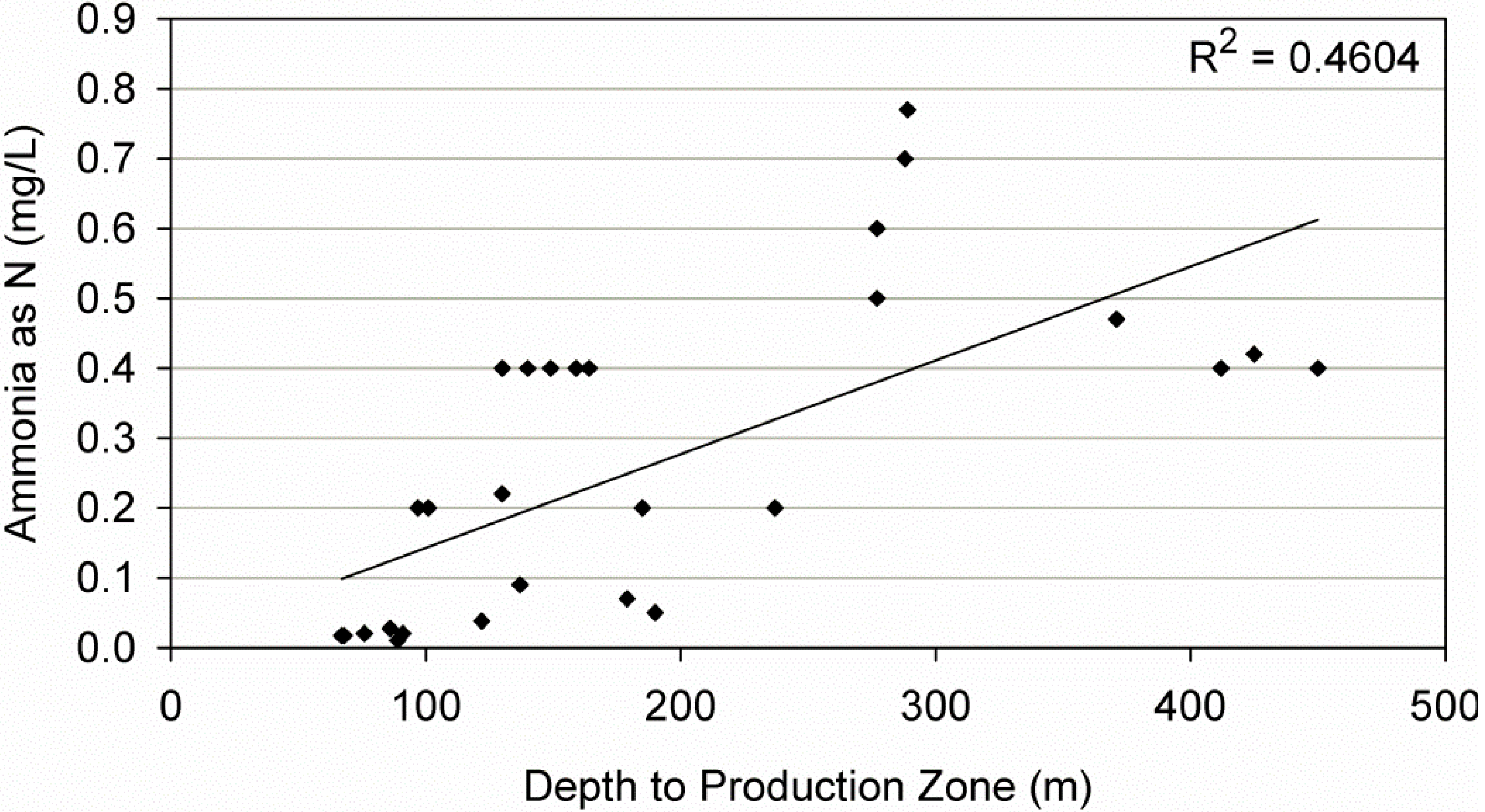
The reaction is known as dissimilatory nitrate reduction to ammonium. It could be seen from Figure 8, as the confining pressure increases (anaerobic conditions), the amount of ammonia in the confined aquifers increases, even exceeding the aesthetic limit of the 0.5 mg/L guideline value [2].

Figure 8. Ammonia in confined aquifers.

Figure 8. Ammonia in confined aquifers.

4.3. Relation of Actual Coliform Detection in Water Supply Wells to GRAM Likelihood

The GRAM calculated likelihood of detection using scores from Table 1, Table 2 and Table 3 are plotted against actual coliform detection frequency for each well in 30 potable water supply systems (Figure 9).

The results show a tendency of increasing detection with increasing likelihood. The fundamental reason for poor co-relation is, in proactive protection, GRAM calculates likelihood of release based on the four attributes given in Table 1 (not based on any actual measurements/detection), and therefore is a measure of release probability rather than actual release. However, coliform detection frequency increases with increasing GRAM risk levels, which are summarised in Table 5.

Figure 9. GRAM likelihood vs. actual coliform detection.

Figure 9. GRAM likelihood vs. actual coliform detection.

Table 5. GRAM risk levels and frequency of coliform detection for 30 groundwater systems; Number of systems in each category is given in brackets.

GRAM Risk Levels	Frequency of Coliform Detection
	Average	Median	Range
Low (15)	0.09	0.04	0–0.45
Medium (4)	0.13	0.08	0.01–0.63
High (11)	0.4	0.37	0–0.96

Table 5. GRAM risk levels and frequency of coliform detection for 30 groundwater systems; Number of systems in each category is given in brackets.

GRAM Risk Levels	Frequency of Coliform Detection
	Average	Median	Range
Low (15)	0.09	0.04	0–0.45
Medium (4)	0.13	0.08	0.01–0.63
High (11)	0.4	0.37	0–0.96

5. Risk Management Case Histories

5.1. Risk Reduction through Changes to Well Designs and Layout

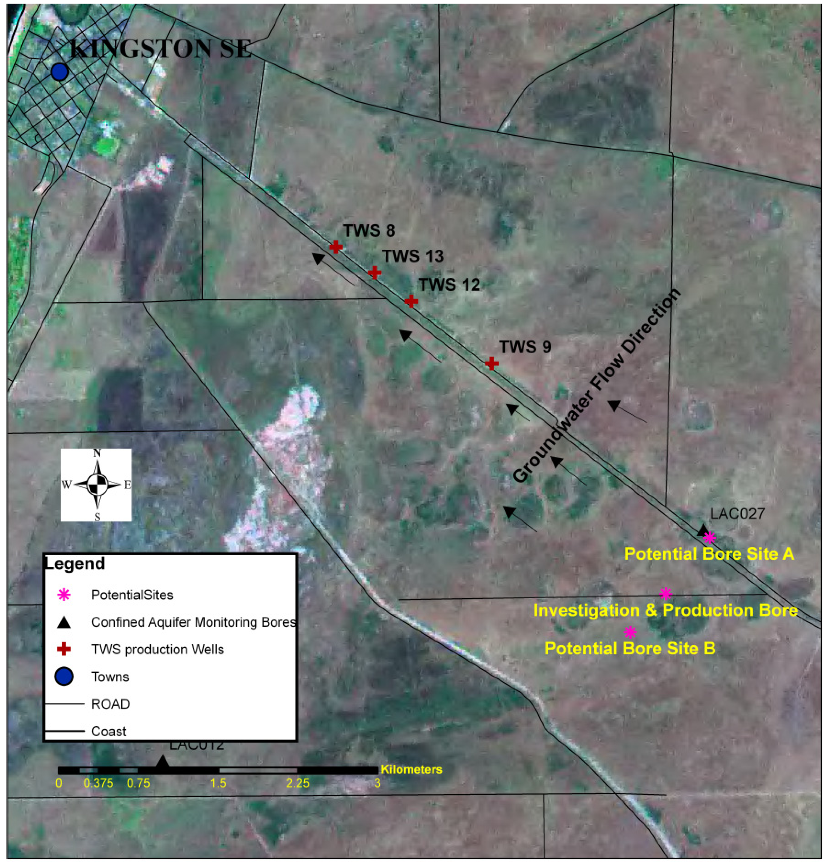
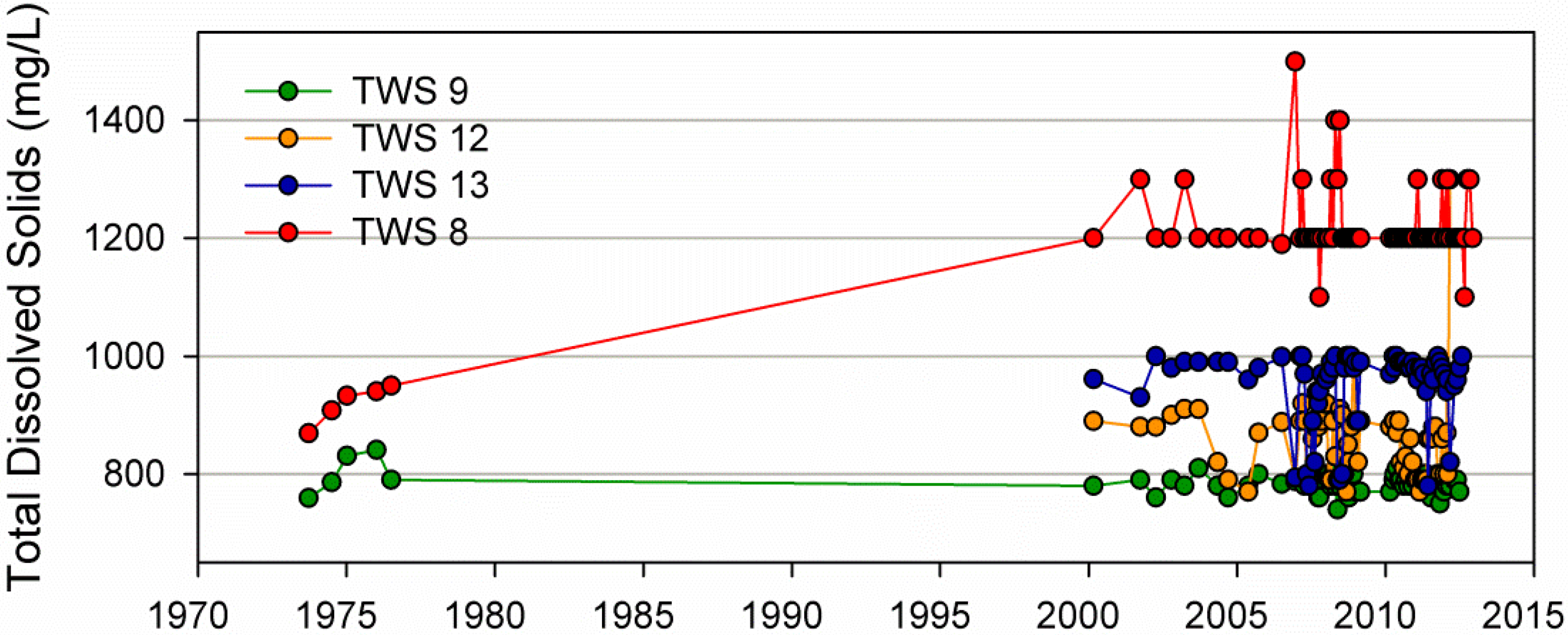
Water supply well design is an important aspect in maintaining groundwater quality and protecting the aquifer. In Kingston SE, four water supply wells were designed along the same flow path, one after the other along a road (Figure 10). On either side of the road is a marsh, linked to the upper Bridgewater Formation aquifer with salinity of 3000–15,000 mg/L. The town water supply wells targets the lower Mepunga Formation confined sand aquifer which contains fresh water of salinity 750–850 mg/L. The location of wells along the flow path is as follows: TWS 9 is the first well, which captures fresh groundwater flow, followed by TWS 12, TWS 13, and finally TWS 8 (Figure 10). Since groundwater flow is progressively reduced in the flow direction from TWS 12, TWS 13 and TWS 8, salinity of the wells progressively increases due to leaking of upper unconfined groundwater (Figure 11). A new wellfield was designed perpendicular to the flow direction, so that each well has individual capture zones in the deeper Dilwyn Formation confined sand aquifer. A new investigation/production well (TWS 15) was drilled into this formation and successfully tested with 40 L/s yield and salinity of 700 mg/L. Salinisation has caused long-term aesthetic impact to the drinking water quality of the township.

Figure 10. Layout of the Kingston South East (SE) wellfield.

Figure 10. Layout of the Kingston South East (SE) wellfield.

Figure 11. Salinity in Kingston SE water supply wells.

Figure 11. Salinity in Kingston SE water supply wells.

The Mepunga Formation is immediately below the Bridgewater Formation and separated by a sandy clay aquitard. Therefore, excessive and permanent drawdown caused by lack of groundwater replenishment due to interception led to downward leakage of brackish water to the production zone. Likelihood of release was assessed using scores from Table 1 (continuous low quantity release with no attenuation, no control or mitigation measures) to be 0.65. A summary of risk assessment for TWS 8 and new investigation/production well (TWS 15) is given in Table 6.

Table 6. Summary of risk assessment for town water supply TWS 8 and TWS 15.

Source and Hazards	Receptor	Consequence	Likelihood of release	Strata vulnerability	Well integrity	Risk level
Aquifer with brackish water: Salinity	TWS 8	5	0.65	0.1	0.3	Medium (0.97)
	TWS 15	5	0.1	0.1	0.1	Low (0.05)

Table 6. Summary of risk assessment for town water supply TWS 8 and TWS 15.

Source and Hazards	Receptor	Consequence	Likelihood of release	Strata vulnerability	Well integrity	Risk level
Aquifer with brackish water: Salinity	TWS 8	5	0.65	0.1	0.3	Medium (0.97)
	TWS 15	5	0.1	0.1	0.1	Low (0.05)

5.2. Risk Reduction through Changes to Well Operational Practice

Good well design and operational practices are critical in fragile groundwater systems. Coffin Bay town water supply relies on a small fresh groundwater lens formed in the upper Bridgewater Formation aquifer. Below this, Tertiary clay and Tertiary sand units contain brackish and saline water. Historically, three wells (TWS 1, TWS 2 and TWS 3) were used, operating 10–12 h per day with pumping rates of 8–12 L/s. Due to TWS 1 being drilled 1 m into the Tertiary clay and excessive pumping, up-conning occurred and the use of the well was ceased in 2005, thus relying on only TWS 2 and TWS 3 for water supply. A rising trend of salinity was noticed in TWS 3, and two additional wells were drilled in 2009 to handle the demand. An analytical model [42] was used to calculate well drawdowns for different pumping scenarios to assess drawdown effect.

A stiff-plastic clay aquitard separating the fresh water lens from the brackish to saline water aquifer has not been tested for vertical leakage. Therefore, based on similar aquitard parameters in adjacent Uley South basin, a vertical hydraulic conductivity of 0.022 m/day was used to calculate vertical leakage due to simulated drawdowns from the analytical model. The result of the risk assessment for pre- and post-implementation of an additional two wells is given in Table 7. In this risk assessment, well integrity is not applicable (NA) as the risk agent is upward leakage of brackish water. Strata vulnerability was set to negligible due to stiff clay layer and the main risk element is therefore caused by well operation (likelihood of release of brackish water). The likelihood of release was set to 0.65 and 0.4 (no attenuation, mitigation or control measures) based on potential leakage reduction from Level 3 to Level 1 from Table 1.

Table 7. Summary of risk assessment for TWS 3: pre- and post-implementation of an additional two production wells.

Source and Hazards	Receptor	Consequence	Likelihood of release	Strata vulnerability	Well integrity	Risk level
Up-coning: Salinity	TWS 3 (pre)	5	0.65	0.2	NA	Medium (0.65)
	TWS 3 (post)	5	0.4	0.2	NA	Low (0.4)

Table 7. Summary of risk assessment for TWS 3: pre- and post-implementation of an additional two production wells.

Source and Hazards	Receptor	Consequence	Likelihood of release	Strata vulnerability	Well integrity	Risk level
Up-coning: Salinity	TWS 3 (pre)	5	0.65	0.2	NA	Medium (0.65)
	TWS 3 (post)	5	0.4	0.2	NA	Low (0.4)

This resulted in a new operational cycle of 5 h with two wells pumping at 5 L/s with a 5 h resting period for recovery. The gradually increasing salinity in TWS 3 was observed from 2004 up until 2009, followed by stable and declining salinity after 2009 (Figure 12).

Figure 12. Coffin Bay TWS 3 salinity.

Figure 12. Coffin Bay TWS 3 salinity.

5.3. Increasing the Time of Residence

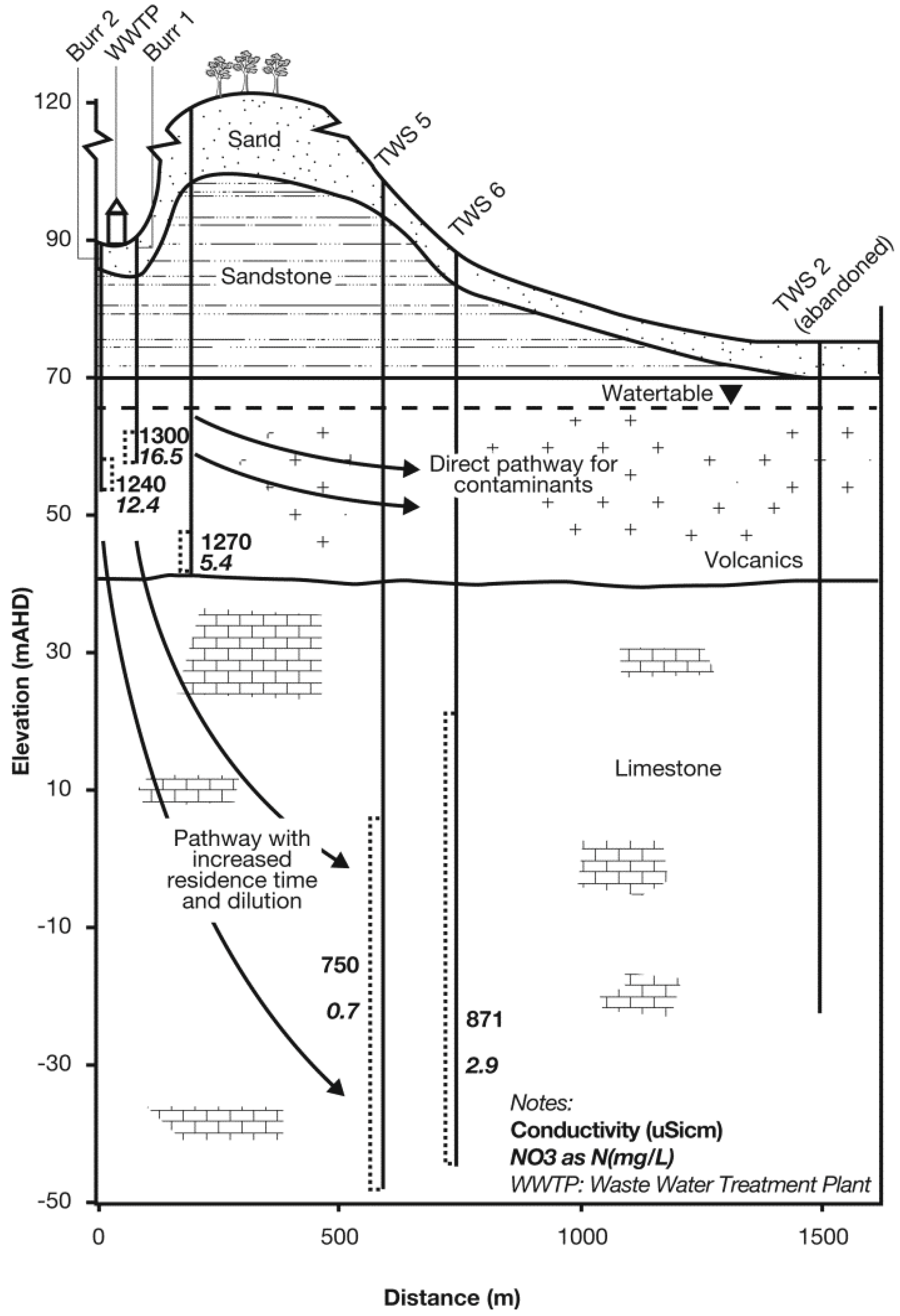
The time of residence for the contaminants and dilution within the aquifer can be used in a beneficial way to minimise risk. At Mount Burr, a waste water treatment plant (WWTP) is located 700 m down gradient of two water supply wells. The WWTP lagoon is known to leak and monitoring wells detected elevated nitrate (as N) up to 16.5 mg/L (Figure 13). Both town water supply wells failed the well integrity test, having failed casing requiring well replacement. Shifting replacement wells to other locations required additional infrastructure costs.

MODFLOW-2000 [43] and particle tracking model MODPATH [44] based groundwater models indicated drawdown curves of water supply wells extend up to 1 km, and that a hydraulic gradient exists towards the production wells. The limestone aquifer’s hydraulic conductivity is 2–5 m/day, and therefore, any pathogens that enter the saturated zone might die off, since a minimum of 375 days is required to reach the production wells at maximum drawdown. Therefore, WWTP induced pathogens were assessed to pose no risk to production wells. The production zones of the replacement wells were set 40 m below the watertable so that nutrients might dilute before reaching the production zones of the new wells. Even though it is possible to model nutrient transport through aquifer systems, this was not followed, as it requires a comprehensive measured data set to obtain reliable results. Therefore, a qualitative judgment was made to set the production zone deeper into the aquifer for maximum attenuation by dilution. This well design has reduced the risk level from Medium to Low level. A summary of risk assessment for failed well (TWS 1) and replacement well (TWS 6) is provided in Table 8.

Figure 13. Mount Burr town water supply wells and waste water treatment plant (WWTP).

Figure 13. Mount Burr town water supply wells and waste water treatment plant (WWTP).

Table 8. Summary of risk assessment for TWS 1 and TWS 6.

Source and Hazard	Receptor	Consequence	Likelihood of Release	Strata Vulnerability	Well Integrity	Risk level
WWTP: Nutrients	TWS 1	5	0.3	0.14	0.7	Medium (1.1)
	TWS 6	5	0.3	0.14	0.1	Low (0.21)

Table 8. Summary of risk assessment for TWS 1 and TWS 6.

Source and Hazard	Receptor	Consequence	Likelihood of Release	Strata Vulnerability	Well Integrity	Risk level
WWTP: Nutrients	TWS 1	5	0.3	0.14	0.7	Medium (1.1)
	TWS 6	5	0.3	0.14	0.1	Low (0.21)

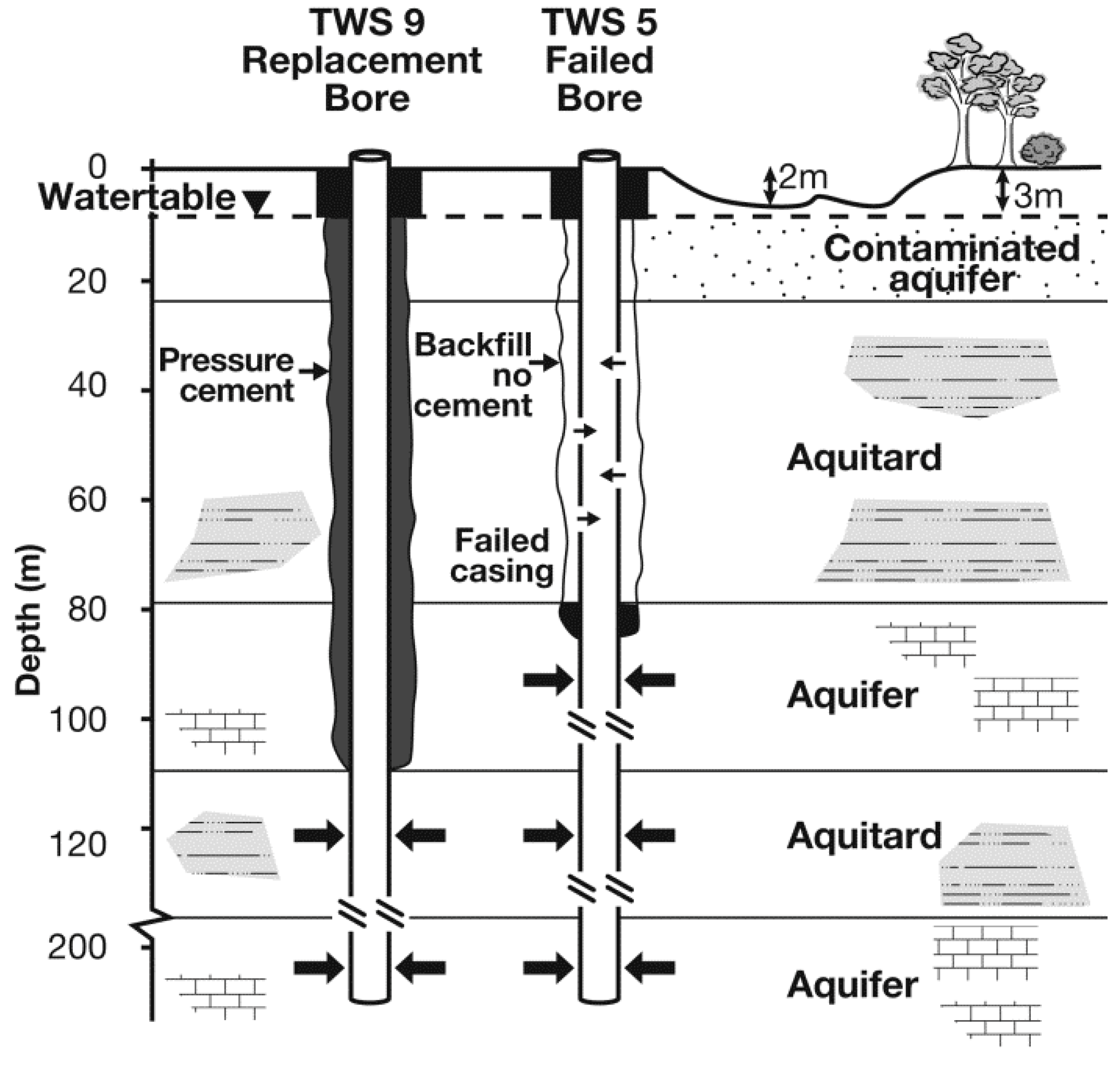
5.4. Risk Reduction through Use of Vertical Flow Barriers

The importance of setting a production zone of the well below an impermeable layer and maintaining well integrity is illustrated in Millicent’s (population 4000) TWS 5. The depth to water in the shallow unconfined Gambier Limestone unit is about 2–3 m. The upper aquifer unit is calcrete, with 1 m of silty soil cover. This results in the upper aquifer having a 0.57 vulnerability index (High vulnerability). However, setting the production zone below stiff clay aquitard of over 20 m thickness results in the vulnerability index being reduced to 0.1 (Negligible). The land use here is predominantly sheep and cattle grazing. A single tree is near the waterhole adjacent to the TWS 5, and therefore, animals flock for shelter at this point. Under these conditions, the likelihood of release of contaminant is 0.62 (most frequently, high quantity or continual low quantity release with low attenuation and no control and mitigation measures in place). The upper part of the aquifer is known to be polluted, having nitrate (as NO₃) levels exceeding 60 mg/L [45]. However, the production zone of TWS 5 has been set below an impermeable clay aquitard layer 80 m from the ground surface (Figure 14).

In 2009, coliform were detected at a frequency of 0.8 of detection, and subsequently, a well integrity test was carried out in 2010. This confirmed that the corroded casing had failed in several locations. The annulus of the well had not been pressure cemented, and failed casing made a pathway of contact with the polluted upper part of the aquifer. A replacement well (TWS9) with PVC casing and pressure cemented annulus was constructed at the site, and is currently supplying coliform free water, despite the fact that an adjacent waterhole is hydraulically connected to the aquifer. For comparison, summary of risk assessments for TWS 5 and TWS 9 are given in Table 9.

Figure 14. Millicent water supply wells.

Figure 14. Millicent water supply wells.

Table 9. Summary of risk assessments for TWS 5 and TWS 9.

Source and Hazards	Receptor	Consequence	Likelihood of release	Strata vulnerability	Well integrity	Risk level
Waterhole: Pathogens, NO3, Ammonia	TWS 5	10	0.62	0.1	0.7	High (4.3)
	TWS 9	10	0.62	0.1	0.1	Medium (0.62)

Table 9. Summary of risk assessments for TWS 5 and TWS 9.

Source and Hazards	Receptor	Consequence	Likelihood of release	Strata vulnerability	Well integrity	Risk level
Waterhole: Pathogens, NO3, Ammonia	TWS 5	10	0.62	0.1	0.7	High (4.3)
	TWS 9	10	0.62	0.1	0.1	Medium (0.62)

6. Conclusions

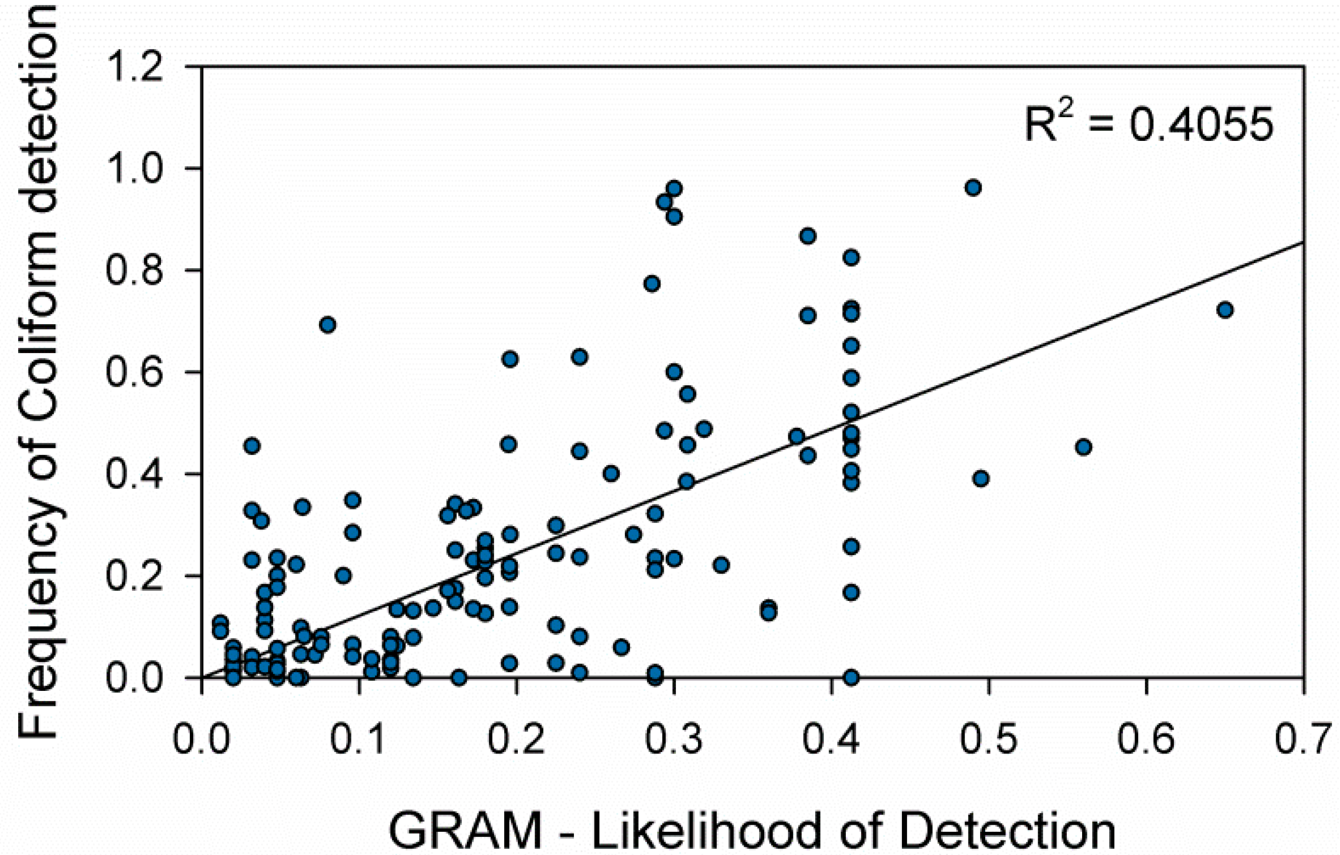
We show that semi-quantitative risk assessment models such as GRAM are useful tools in groundwater risk assessments utilizing a multi-barrier approach. In the multi-barrier approach, identification of the weakest barrier is necessary to enable effective risk management. In this study, groundwater vulnerability and well integrity are incorporated to the pathway component of the risk equation. Risk levels resulting from GRAM evaluation compared well to the indicator bacterium, total coliform detections. In our case studies, most high risk systems are related to poor well construction and casing corrosion rather than land use. Risk management actions, including changes to well designs and well operational practice, designs to increase time of residence, and setting the production zone below identified low permeable zones, provide additional barriers to protect and secure the water supply. The highlight of the risk management element is well integrity testing using downhole geophysical methods.