Article

An Approach Using a 1D Hydraulic Model, Landsat Imaging and Generalized Likelihood Uncertainty Estimation for an Approximation of Flood Discharge

1
Department of Civil Engineering, Inha University, 100 Inha-ro, Nam-gu, Incheon 402-751, Korea
2
School of Civil Engineering, Purdue University, 550 Stadium Mall Drive, West Lafayette, IN 47907, USA
3
Department of Biological & Agricultural Engineering, Texas A&M University, College Station, TX 77843, USA
4
School of Urban and Civil Engineering, Hongik University, Seoul 121-791, Korea
*
Author to whom correspondence should be addressed.
Water 2013, 5(4), 1598-1621; https://doi.org/10.3390/w5041598
Submission received: 31 July 2013 / Revised: 23 September 2013 / Accepted: 24 September 2013 / Published: 7 October 2013
(This article belongs to the Special Issue Advances in Remote Sensing of Flooding)

Abstract

:
Collection and investigation of flood information are essential to understand the nature of floods, but this has proved difficult in data-poor environments, or in developing or under-developed countries due to economic and technological limitations. The development of remote sensing data, GIS, and modeling techniques have, therefore, proved to be useful tools in the analysis of the nature of floods. Accordingly, this study attempts to estimate a flood discharge using the generalized likelihood uncertainty estimation (GLUE) methodology and a 1D hydraulic model, with remote sensing data and topographic data, under the assumed condition that there is no gauge station in the Missouri river, Nebraska, and Wabash River, Indiana, in the United States. The results show that the use of Landsat leads to a better discharge approximation on a large-scale reach than on a small-scale. Discharge approximation using the GLUE depended on the selection of likelihood measures. Consideration of physical conditions in study reaches could, therefore, contribute to an appropriate selection of informal likely measurements. The river discharge assessed by using Landsat image and the GLUE Methodology could be useful in supplementing flood information for flood risk management at a planning level in ungauged basins. However, it should be noted that this approach to the real-time application might be difficult due to the GLUE procedure.

1. Introduction

It is recognized that floods are one of the most severe and frequent globally-occurring natural hazards which can limit human activities, and, in this respect, continuous efforts and investments are leading to a better understanding of the nature of floods. Among flood properties, the measurement of river discharge provides fundamental information for flood risk management, and gauging stations play a critical role in collecting data of discharge, water level, and water quality, which are essential information to address real time flood forecasting and reservoir operation. Good gauging station networks allow flow estimations for various return periods, using extreme value statistics based on long gauge records [1,2]. However, the use of subjectivity in relation to the decision of theoretical probability distribution functions for data and the inference methods for parameters, can critically affect the estimation of flow for a rare extreme event [3,4,5,6]. Moreover, lack of the observed data gives a critical difficulty in planning flood risk through computer modeling, which requires hydrologic data, including discharge data that cannot be easily obtained in ungauged basins.
Flood discharge estimation gives significant contribution in identifying the design flood as fundamental information for flood risk management at a planning level. Therefore, flood estimation has been conducted in ungauged basins using hydrologic approaches such as regionalization techniques and conceptual models. Regionalization techniques are used to apply hydrologic information retrieved from neighboring basins, where the required data are collected, to a targeted ungauged basin [7,8,9,10]. The techniques are based on the hydrologic homogeneity between neighboring gauged and ungauged regions. Sometimes, the rational method is also used. The rational method is a simple transformation process of rainfall into runoff using the relationship between the runoff coefficient, rainfall intensity, and basin size [11]. However, estimating the runoff coefficient is difficult because it can vary depending on the rainfall intensity or the geometric properties of a basin. For these reasons, regionalization techniques and conceptual models can only estimate the design flow, but have difficulties in considering distinct attributes for individual flood events.
The availability of spatio-temporal data using remote sensing devices can provide an information-rich environment for analyzing flood properties [12,13,14]. In particular, satellite remote sensing imagery with specific cycles (e.g., daily or every 16 days), can be used to detect the spatiotemporal changes of floods [15,16]. Geographic information systems (GIS), also help to build a database, covering spatiotemporal flood evidence obtained from satellite imagery, and allows easy access for the analysis of flood properties with other geographic data (e.g., digital elevation models and land use maps). As a result, the extent of a flood or the water surface elevation obtained from satellite imagery, have played a role in the calibration of data in hydrologic and hydraulic modeling [17,18,19,20]. In addition of obtaining data, there have been great efforts to improve the quality of GIS and RS data in order to extend their applicability [21,22,23,24]. Due to these advantages, the application of satellite imaging and GIS has been considered as one of the most practical and cost-effective approaches for hydraulic and hydrologic analysis in data-poor, or even in ungauged basins, without limitations of spatial boundaries.
The generalized likelihood uncertainty estimation (GLUE) method, proposed by Beven and Binley [25], is one of the first methods to represent prediction uncertainty in hydrologic and hydraulic modeling. The GLUE method uses the Monte Carlo simulations in conjunction with Bayesian theory to produce parameter distributions conditioned on available data and associated uncertainty bounds. The parameter distributions are generated based on multi-parameter sets that can produce acceptable model outputs in comparison with observed data. The criterion for an acceptable model is based on the definition of a user-specified likelihood function. The GLUE method has found widespread implementation in various studies related to uncertainty analysis in environmental, hydraulic, and hydrologic modeling, including flood mapping [26,27,28]. However, the use of formal and informal likelihood measures for model calibration and uncertainty estimations have been debated in certain literatures [29,30,31]. Here, formal and informal mean statistical likelihood measure and non-statistical, respectively. In this study, we acknowledge limitations related to the subjectivity of GLUE’s informal likelihood measure, but assume that the GLUE methodology has the practical potential for incorporating the uncertainty in flood modeling in a data-poor environment, where a formal likelihood is not available. However, the use of the GLUE methodology in flood discharge estimation can make it difficult to forecast flood discharge in real time application.
Informal likelihood measures to be used in the GLUE methodology can be estimated by using flood information derived from remote sensing and water level information. In this context, the objectives of this study are to: (1) identify the flooded area and the water surface elevation from satellite imagery (Landsat TM); (2) propose a methodology for flood discharge estimate by using satellite imagery and GLUE; and (3) verify the approximate flood discharge for different informal likelihood measures using the observed discharge from gauge stations. These three objectives are accomplished with the use of satellite image processing, 1D hydraulic modeling, and the informal likelihood measurement estimation for two study reaches in the United States, including a reach along the Missouri River near Nebraska City, Nebraska, and the Wabash River near Montezuma, Indiana. The selected case studies are characterized by the presence of gauged sections where discharge data are available and are used as a benchmark for verifying the discharge values provided by the proposed methodology.

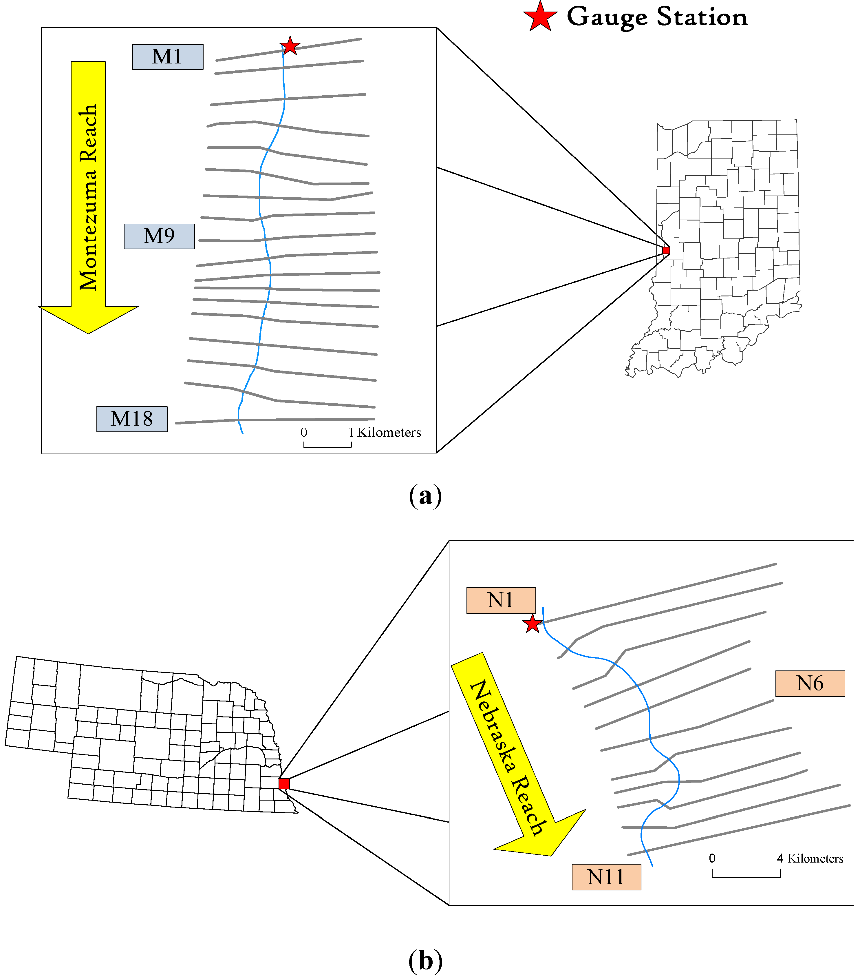
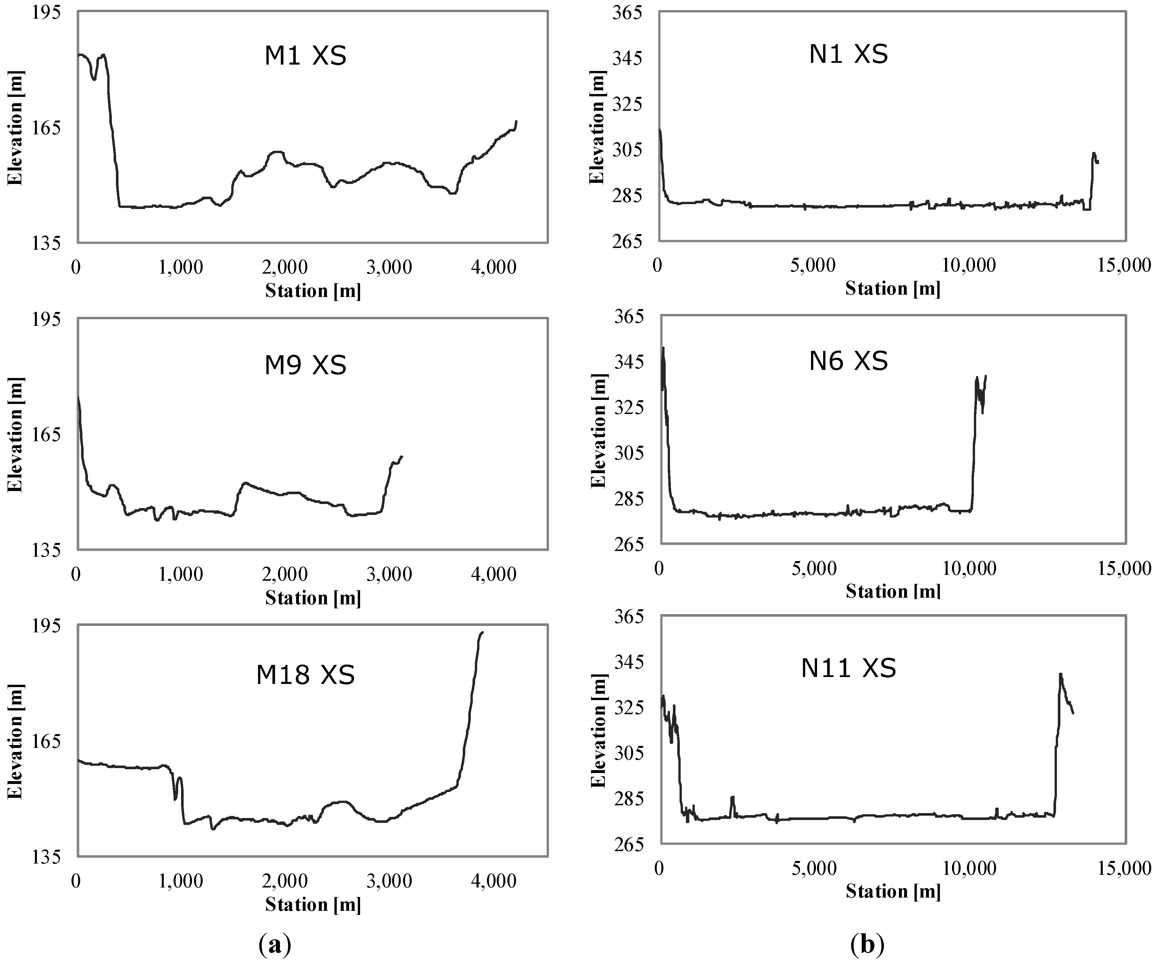
2. Study Area and Data Set

Two river reaches are selected as case studies: one along Missouri River near Nebraska City, Nebraska, USA, henceforth referred to as “Nebraska reach”, and another along the Wabash River near Montezuma, Indiana, USA, named as “Montezuma reach”, as shown in Figure 1. The two reaches are selected because of the difference in their physical conditions, i.e., in their geometry, size, and topography (Table 1). Satellite imagery taken by the Landsat 5 Thematic Mapper (TM) imaging sensors are available from the USGS Landsat Missions [32] for flood events that occurred after 1982, including the ones corresponding to the catastrophic floods that occurred on 11 June 2008 in Indiana, and on 9 July 2011, in Nebraska.
Figure 1. Study reaches. (a) The Wabash River at Montezuma, IN, USA (The Montezuma reach); (b) The Missouri River at Nebraska City, NE, USA (The Nebraska reach).
Water 05 01598 g001
Table 1. Geo-morphological properties of the two selected river reaches for hydraulic modeling.
Study ReachRiver length (km)Mean bed slope (m/km)Number of cross-sectionMean width of cross-section (km)Mean spacing cross-section (km)
Montezuma90.25183.610.53
Nebraska190.211112.841.90
In this study, the use of Hydrologic Engineering Center-River Analysis System (HEC-RAS), a 1D hydraulic model, is justified because the flood extent on the selected Landsat imagery distributes in both of the main channel and floodplain. The geometric data for HEC-RAS consist of eighteen cross sections for the Montezuma reach, and eleven cross sections for the Nebraska reach is commonly extracted from a 10 m × 10 m resolution USGS digital elevation model (DEM), by using HEC-geoRAS. The Manning’s n values for the HEC-RAS model are extracted from the National Land Cover Database 2001 [33]. As shown in Table 2, Moore [34] assigned Manning’s n roughness coefficients for each land use category in NLCD 2001, based on established literature [35,36].
Table 2. Manning’s n values for 2001 National Land Cover Database (NLCD) classification.
2001 NLCD ClassificationManning’s nSource
MinimumNormalMaximum
Open Water0.0250.0300.033[35]
Developed, Open Space 0.0100.0130.160[36]
Developed, Low Intensity 0.0380.0500.063[36]
Developed, Medium Intensity0.0560.0750.094[36]
Developed, High Intensity 0.0750.1000.125[36]
Barren Land 0.0250.0300.035[35]
Deciduous Forest0.1000.1200.160[35]
Evergreen Forest0.1000.1200.160[35]
Mixed Forest0.1000.1200.160[35]
Scrub/Shrub0.0350.0500.070[35]
Grassland/Herbaceous0.0250.0300.035[35]
Pasture/Hay0.0300.0400.050[35]
Cultivated Crops0.0250.0350.045[35]
Woody Wetlands0.0800.1000.120[35]
Emergent Herbaceous Wetland0.0750.1000.150[35]
Each reach has distinct topographic and geomorphic settings which provide good test beds for comparison: The Wabash River, one of the major rivers in Indiana, drains to the Mississippi River, and another reach, the White River, drains to Wabash River. The selected Montezuma reach along the Wabash River is relatively straight and has a length of about nine kilometers. The floodplain of the Montezuma reach is rough and bumpy and is in a relatively U-shaped valley (Figure 2a). The Missouri River is the longest river (3767 km) in North America, and enters the Mississippi River. The selected Nebraska reach along the Missouri River meanders, and is about 19 km long. It has a flat floodplain and lies in a relatively rectangular valley (Figure 2b).
Discharge data are available at gauged sections, which are only used for verifying the methodology developed in this study. The discharge data available are from gauge stations USGS 03340500 [37] for the Montezuma reach, and USGS 06807000 [38] for the Nebraska reach (Table 3). In addition, both gauge stations provides discharge and gauge height for peak flow as well as daily, monthly, and annual stream flow.
Table 3. The observed discharge at USGS gauge stations for flood discharge on Landsat and peak flow in a flood event.
Study ReachUSGS gauge stationFor flood discharge on Landsat imageryFor a peak flow of the flood event
Date of Landsat imageDischarge at gauge station (m3/s)Date of peak flowDischarge at gauge station (m3/s)
Montezuma0334050011 June 200814508 June 20082197
Nebraska068070009 July 201160317 July 20116258
Note: the peak flow belongs to a flood event including the flood discharge on Landsat image.
Figure 2. Geometric shape of cross-sections for study reaches. (a) Montezuma reach; (b) Nebraska reach.
Water 05 01598 g002

3. Methodology

The proposed methodology involves the following steps: (1) identifying the flooded area from Landsat 5 TM satellite imagery using Iterative Self-Organizing Data Analysis (ISODATA); (2) running Monte Carlo simulations with the HEC-RAS model; and (3) approximating the flood discharge using different likelihood measures in the GLUE framework. A brief description of each process used in our methodology follows.

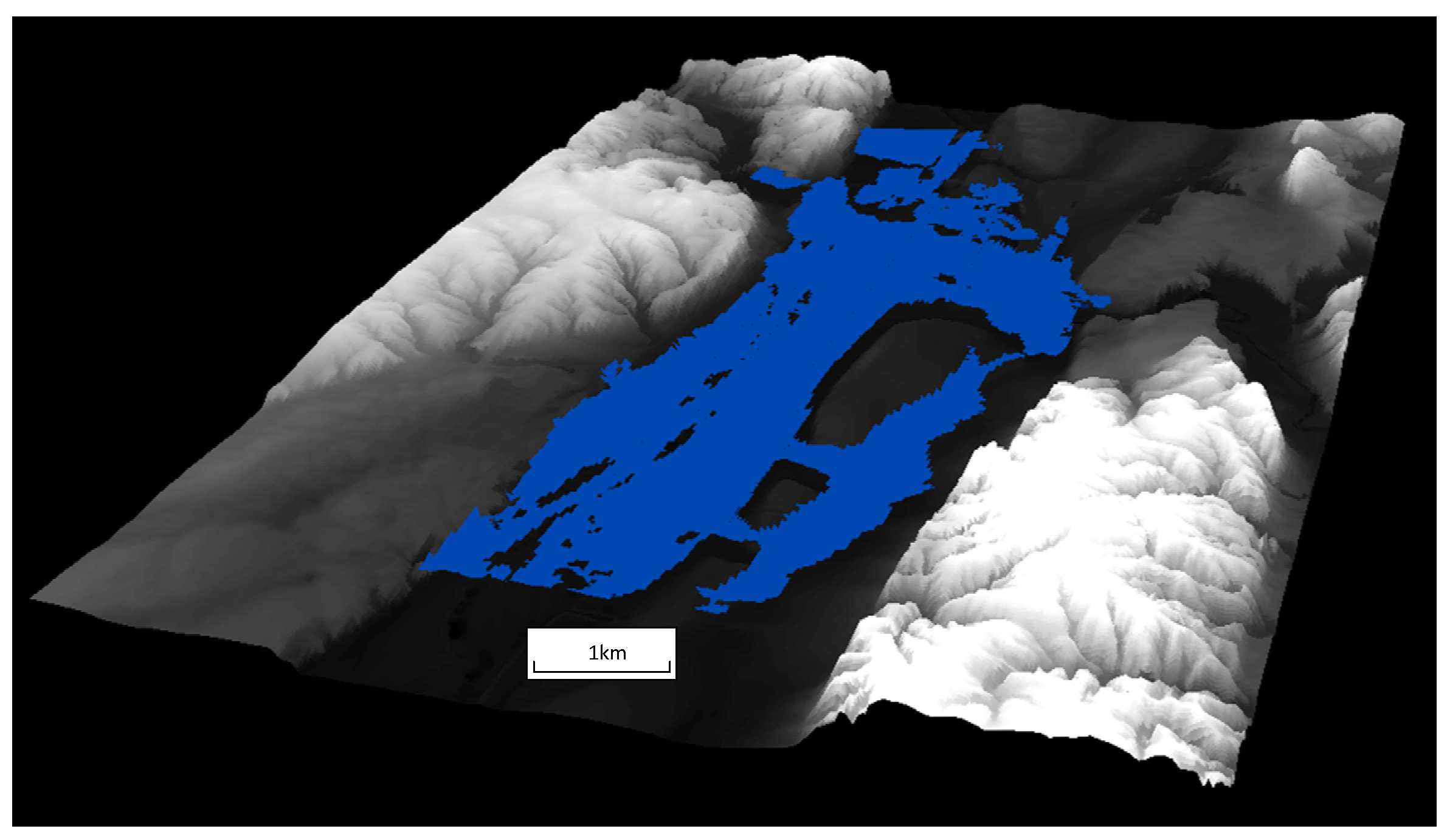
3.1. Extraction of the Observed Data from Landsat 5 TM Satellite Imagery

Image classification categorizes values, which indicate specific properties of pixels in a digital image. There are two main methods of classification used for image processing: supervised classification and unsupervised classification. In this study, the process of extracting the water-body from Landsat imagery is conducted using the image processing algorithm ISODATA (Iterative Self-Organizing Data Analysis), which is one of the unsupervised classification methods that uses cluster algorithms to categorize unknown pixels in the image data, without any foreknowledge of the classes [39,40,41,42,43]. In the processes of ISODATA, a number of points indicating cluster centers are randomly placed on the imagery. The pixels are then located within the given Euclidean distance from the placed points, and a cluster is developed. If the standard deviation for the pixel values in a cluster is greater than a certain threshold, the clusters are split, and if the distance between two clusters is less than the threshold, the clusters are merged. The iterative new cluster centers work as a standard to further divide or merge the cluster in the next iteration. Iterations are performed until: (1) the mean distance between adjacent clusters falls to a threshold in a successive iteration; or (2) the maximum number of iterations is reached. However, it should be noted that there are a few subjective decisions, which need to be made, such as the number of classifications and the number of iterations when using ISODATA. In this study, ISODATA classification is performed for 20 classes and 3 iterations [44].
Landsat 5 TM image has seven spectral bands with different wavelengths, and the resolution of all bands is 30 m, except band 6 with a resolution of 120 m. Bands in Landsat imagery can also be differently combined to classify a specific category, such as a water-body, urban land and farmland. In this study, the ISODATA technique was applied to a combination of the spectral bands 1, 4, and 7 of the Landsat 5 TM image, which was categorized into the 20 groups of land use. This specific combination of the spectral bands is considered for the water-body extraction due to the following reasons: (1) blue light (band 1) with the shortest wavelength penetrates clear water; (2) near infrared (band 4) is strongly absorbed by water, and reflected for soil and vegetation; and (3) mid infrared (band 7) has the distinct nature of absorption of water and reflectance for soil and rock [45]. The classified groups are then compared with the satellite imagery and visible spectral bands (bands 1–3), and the colors placed in water-bodies such as lakes, rivers, and reservoirs are then selected as the water-bodies to be extracted from the imagery. Among the selected clusters, ones, which are falsely classified as water-bodies were manually removed, compared with orthography data, and the rest are merged using the GIS tool. In this study, the water-bodies extracted are considered as a flood inundation map for a flood event, and are used to estimate the water surface elevation at each cross-section with DEM. The flood inundation map and the water surface elevation are then used as observations to estimate the likelihood measures in the approximation of flood discharge using the GLUE methodology.

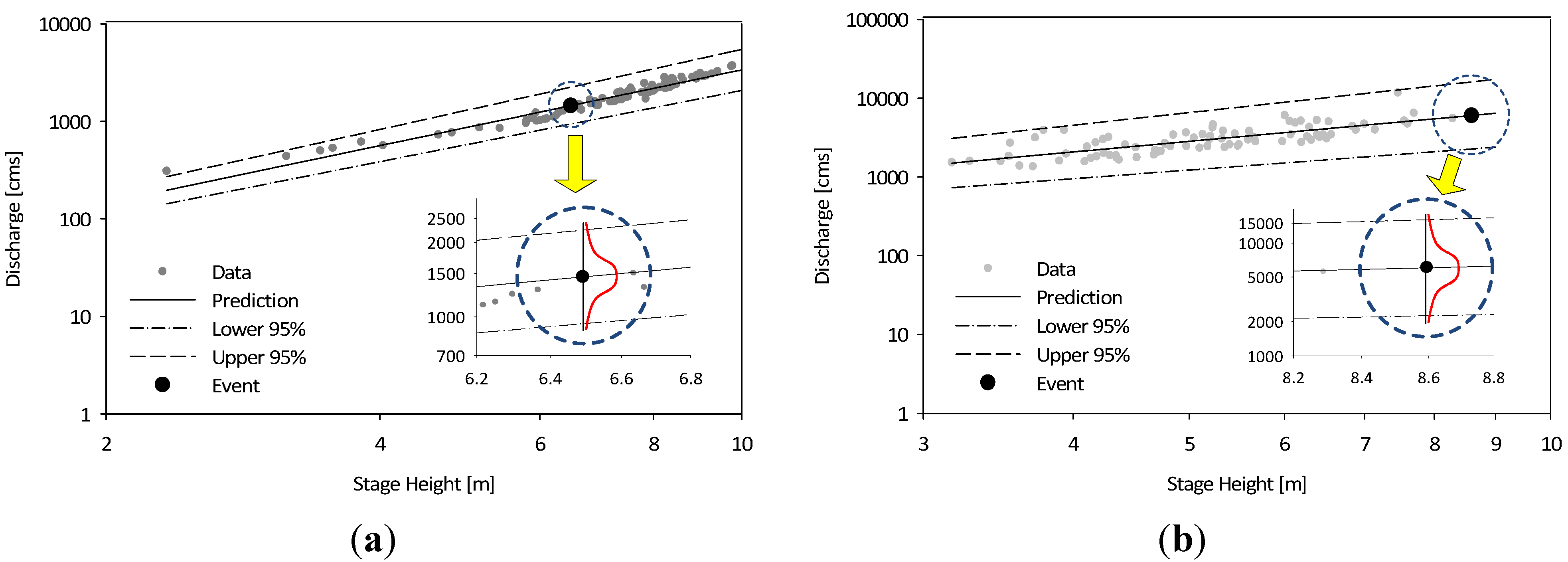
3.2. Approximation of Flood Discharge Using HEC-RAS and the GLUE Methodology

3.2.1. Monte Carlo Simulation Using HEC-RAS

The Hydrologic Engineering Center-River Analysis System (HEC-RAS) is a one-dimensional (1D) model developed by the Hydrologic Engineering Center (HEC), of the United States Army Corps of Engineers (USACE) [46]. The HEC-RAS has the ability to simulate water surface elevation for both steady and unsteady flow conditions in a river channel. Water surface elevations using HEC–RAS are calculated using the energy equation [Equation (1)] and the Manning’s equation [Equation (2)]:
Water 05 01598 i001
where: Y1, Y2 are the depth of water; V1, V2 are the average velocities; Z1, Z2 are the elevation of the main channel; α1, α2 are the velocity weighting coefficients; g is the gravitational acceleration; and he is the energy head loss. In addition, 1 and 2 refer to the upstream and downstream cross section, respectively.
Water 05 01598 i002
where, n is manning’s roughness coefficient; A is the flow area; Sf is the friction slope; and R is the hydraulic radius.
In this study, the hydraulic model HEC-RAS is used assuming that the main river and the floodplains can be simulated as a single channel and that the floodplain only provides a path of flow parallel to the river centerline not acting as a storage area. As with all the hydraulic models, HEC-RAS needs boundary conditions and input data, including cross-section geometry, roughness coefficients, and river discharge. The HEC-RAS needs boundary conditions and input data, including cross-section geometry, roughness coefficients and flow. HEC-GeoRAS, a GIS tool, helps with preprocessing to run the HEC-RAS model. The HEC-GeoRAS can extract the geometry of digitized cross sections with DEM, and export this geometric information to HEC-RAS.
In Monte Carlo simulations using HEC-RAS, A total of 10,000 HEC–RAS simulations are conducted by assuming a steady-state flow condition for each study reach. The model set-up is performed as follows: (1) Discharge is considered as a single input to the model, and, thus, only one random discharge value is generated to conduct one simulation; (2) The prior probability distribution function (PDF) of unknown discharge are assumed as a uniform because there is no available information on discharge in places where no gauge station exists [47,48,49]; (3) The random discharge for the Monte Carlo simulation is uniformly generated in ranges from 100 m3/s to 5000 m3/s for the Montezuma reach, and from 1000 m3/s to 10,000 m3/s for the Nebraska reach. Here, the ranges of discharge for both study reaches are determined to sufficiently cover the discharge on the target flood events, by considering the flood extend width and the water depth obtained from satellite imagery and DEM; (4) Manning’s n value is generally considered as a primary parameter in calibrating HEC-RAS [50,51]. However, in this study, the roughness coefficients extracted from NLCD 2001 (Table 2) are used for calculation of the water surface elevation without calibration of the model, due to the assumption that there is no gauged information regarding the discharge relationship. Downstream boundary condition is represented by normal depth.

3.2.2. Approximation of Flood Discharge Using the GLUE Methodology

The concept of the GLUE methodology is the basis of the Hornberger-Spear-Young (HSY) global sensitivity analysis [52,53], which involves Monte Carlo simulations using different datasets randomly selected from a feasible range. The GLUE methodology has the objective of classifying behavioral and non-behavioral models with feasible parameter datasets [25]. The results from Monte Carlo simulations are used to calculate likelihood measures, which describe the degree of fitness between the simulations and the observations. Generally, likelihood measures in the GLUE methodology are based on the Bayes equation [Equation (3)], and are estimated using several likelihood functions, including the inverse of the sum of the squared error, the inverse of the sum of absolute error, and the Nash-Sutcliffe efficiency:
Water 05 01598 i003
where: PL is posterior likelihood values; and X is the value of x simulated by model; L[M(Θ,I)] is a likelihood measure by model prediction (M) for given parameter (Θ) and set of input data (I); Pi is a penalty function; i is iteration; and r is a cut-off threshold.
As shown in Equation (3), a high likelihood measure means a good fit between the simulation and the observations, and vice versa. The classification of either a behavioral model or a non-behavioral model among likelihood measures is determined by the user-specific cutoff threshold. However, there is no obvious definition or criteria to select the cut-off threshold for classifying simulations into behavioral and non-behavioral datasets [54]. The cut-off threshold can be determined in terms of an absolute value (e.g., Nash Sutcliffe Efficiency >0.5), or as a percentage of total simulation (e.g., a top 30% of the 10,000 likelihood measures sorted from the highest to the lowest value). The selected likelihood measures as behavioral models are then rescaled from 0 to 1 by Equation (4):
Water 05 01598 i004
where, the ith rescaled likelihood measure (RSLi) is calculated by the ith likelihood measure (Li), the minimum likelihood measure (LMIN), and the maximum likelihood measure (LMAX).
The rescaled likelihood measures are used to obtain the probability density function (PDF) and cumulative density function (CDF) of the output prediction. Generally, the median of the CDF based on the rescaled likelihood measures, represents the deterministic model prediction, and the uncertainty bound can be represented with the 90% confidence interval bounded by 5% and 95% confidence levels [55,56,57]. In this study, the behavioral model is based on a cut-off threshold, by taking the top 30% of likelihood measures [58], and is used to estimate 90% of uncertainty bounds for approximation of a flood discharge.
In this study, the informal likelihood measure in the GLUE methodology is based on water surface elevations and continuous flood extents obtained from Landsat imagery and GIS. Equation (5) means the sum of the squared error (SSE) of the water surface elevations used in the GLUE methodology to calculate likelihood measures (E likelihood measure), using the difference between the observations and the simulations in flood modeling [59,60,61,62].
Water 05 01598 i005
where, Em,i and Eo represent the ith iteration of the modeled water surface elevation and the observed water surface elevation, respectively, for the jth among a total N of cross-sections.
Despite the limitation that water surface level at gauge stations as an observation cannot capture the spatial distribution of flooding, the water surface level still plays an important role, within a spatial data-poor area, in estimating the likelihood measure for the observed flood inundation maps, (due to the lack of observed flood inundation maps). In recent decades, the extent of flood inundation extracted from satellite imagery has been used as observations for capturing the spatial uncertainties in flooding [44,63,64,65]. F-statistic [Equation (6)] is a typical likelihood function using the spatial distribution of flooding, which means the goodness of fit between the observed flood area and the simulated flood area, based on their overlapped area [66,67,68,69,70].
Water 05 01598 i006
where Ao indicates the observed inundation area; Ap refers to the predicted flood inundation area; and Aop represents an overlap of both the observed and the predicted inundation areas.
In this study, the simulated flood area (Ap) of Equation (6) is based on results obtained from HEC-RAS, which provides water surface elevations only along cross sections. To produce the flood inundation area from these discrete model outputs, the DEM is subtracted from the water surface area, which is derived by the inverse distance weight (IDW) interpolation of the water surface elevations at each cross section. Equation (7) (EF likelihood measure) is a likelihood measure proposed in this study, which considers both the vertical and spatial differences due to the availability of the water surface elevation and the flood extents as observations.
Water 05 01598 i007
where, EF indicates the coupled likelihood measure based on the rescaled E likelihood measure (RSLE) and the rescaled F-statistic (RSLF); i is iteration; and α is the weight coefficient ranging from 0 to 1.
In this study, the value of α in Equation (7) is selected with 0.5, under the condition that the vertical and spatial effects of likelihood measure are the same on the extracted flood inundation map. As mentioned in the Introduction, the use of informal likelihood measure in the GLUE methodology has been criticized due to its subjectivity, but different informal likelihood functions, based on the water surface elevation and the extent of flood inundation, can be used to approximate flood discharge bounds, due to the unavailability of formal likelihood measure in this study.

4. Results and Discussion

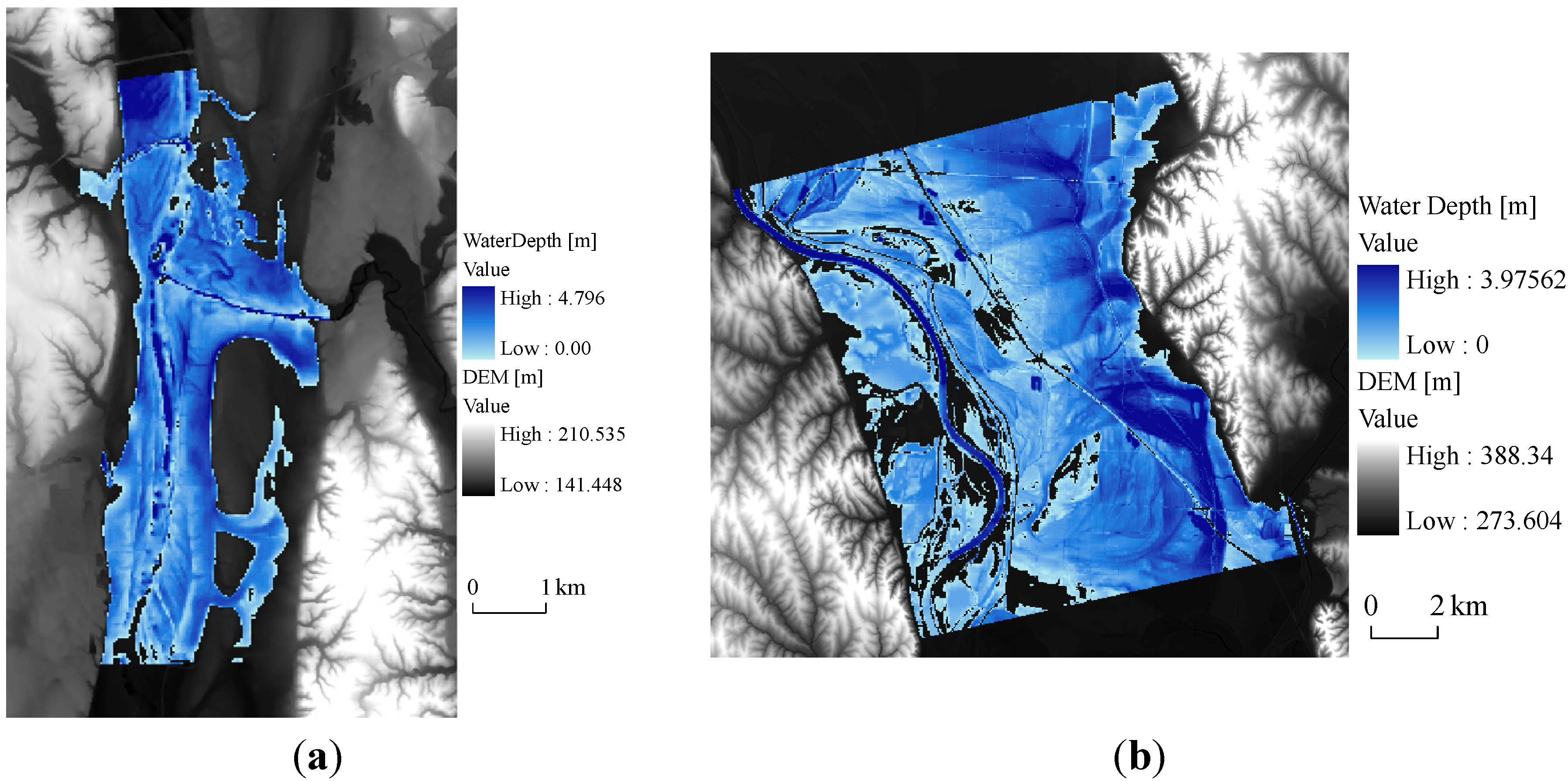
4.1. Extraction of the Observed Data from Landsat 5 TM Satellite Imagery

The water-bodies for both study reaches are extracted from spectral imageries consisting of bands 1, 4, and 7 of the Landsat 5 TM data. Figure 3 shows the water bodies extracted using the ISODATA technique. Considering the distribution of the flood extent for both study reaches, the result shows that the flow direction does not follow the original river center for extreme flood events because the flood streamflow flowed over the main channel and the floodplain, while the original flow direction in only main channel located inside floodplain is relatively meandering (Figure 4). This restrains the application for high flow conditions using the model calibrated for low flow conditions, because the downstream slope of flow can be changed by water level corresponding to the magnitude of streamflow. The total area of the extracted water-body is 13.2 km2 for the Montezuma reach and 105.0 km2 for the Nebraska reach, and is used as the observed flood inundation maps to estimate the F likelihood measures in the GLUE methodology.
Figure 3. Three-dimensional representations of water-body overlaid on DEM extraction using ISODATA (Montezuma reach, 11 June 2008). Water-body (blue solid) extracted from Landsat image on DEM.
Water 05 01598 g003
Figure 4. Intersection points for reading water surface elevation from DEM (Montezuma reach, 11 June 2008).
Water 05 01598 g004
Another observation data obtained from Landsat image is the water surface elevation at each cross section used in the 1D model. To derive the water surface elevation from DEM, the intersection points between boundaries of the flood inundation extents and the cross-sections are required, because the water surface elevation simulated by HEC-RAS is calculated for each cross-section. The use of GIS enhances the accuracy of point locations and reduces the time in finding the intersection points and in reading the elevations of those points from the DEM. Figure 4 shows the cross-sections, extracted flood extent boundary, and intersections between the two overlaid features on DEM of the Montezuma reach. The results for the observed water surface elevations are shown in Figure 5. As a result, there is fluctuation in elevations of intersection points belonging to a cross-section. Thus, an observed water surface elevation at each cross-section is determined by taking an average of elevations of intersection points at the cross-section. Points at which the water-body is too small, or which cloud covers completely, are excluded in the calculation of the average elevation. For 18 cross-sections of the Montezuma reach, the average elevations range from 144.47 m to 148.00 m, and the standard deviations range from 0.03 m to 2.62 m. In the case of the Nebraska reach, the average elevations are in the range of 277.45 m to 281.27 m, and the standard deviations are between a minimum of 0.82 m and a maximum of 1.42 m, respectively. As a result obtained from Landsat and DEM, the Montezuma reach, with its relatively narrow and rough floodplain has a greatly fluctuating water level from upstream to downstream, compared with the Nebraska reach which has a wide and flat floodplain. From these results, the coarse resolution of Landsat imagery produces relatively greater uncertainty in reading the elevation from DEM in a small reach than in a large reach. In particular, compared with the Nebraska reach, rough floodplain of the Montezuma reach (Figure 2) would lead to high storage effect or water level deviation from the extracted flood inundation and DEM because the coarse resolution of Landsat data and the horizontal and vertical error of DEMs can be more propagated to the rough floodplain than to flat floodplain. With coarse resolution of Landsat data and horizontal and vertical errors in DEM, various uncertainty sources, such as the image processing technique, and the geometric characteristics in the processes of flood information acquisition should be considered to improve the accuracy of the flood information obtained from GIS and RS data.
Figure 5. The water surface elevation (WSE) obtained from Landsat image and water surface elevation from Monte Carlo (MC) simulations. (a) For the Montezuma reach; (b) For the Nebraska reach.
Water 05 01598 g005

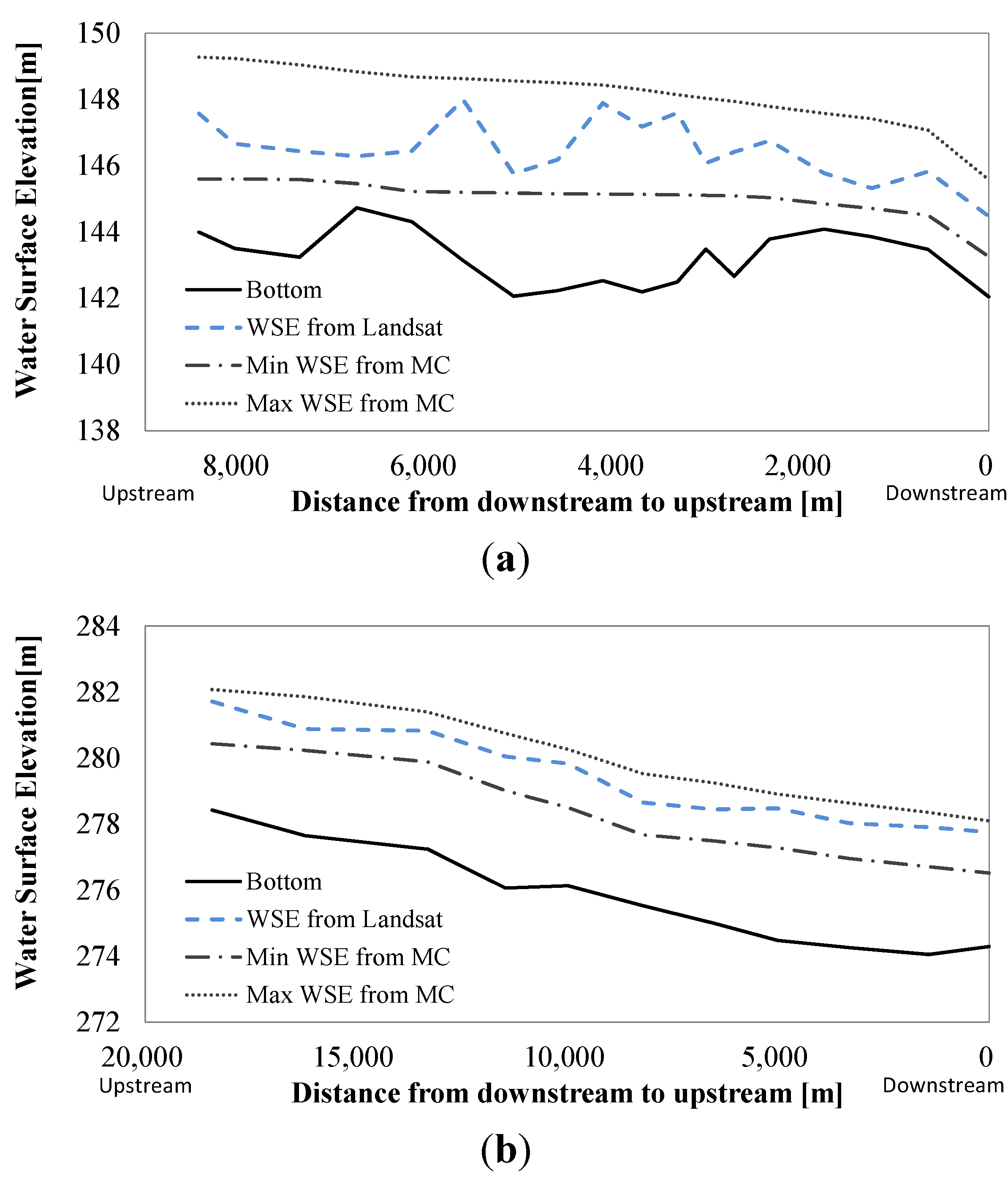
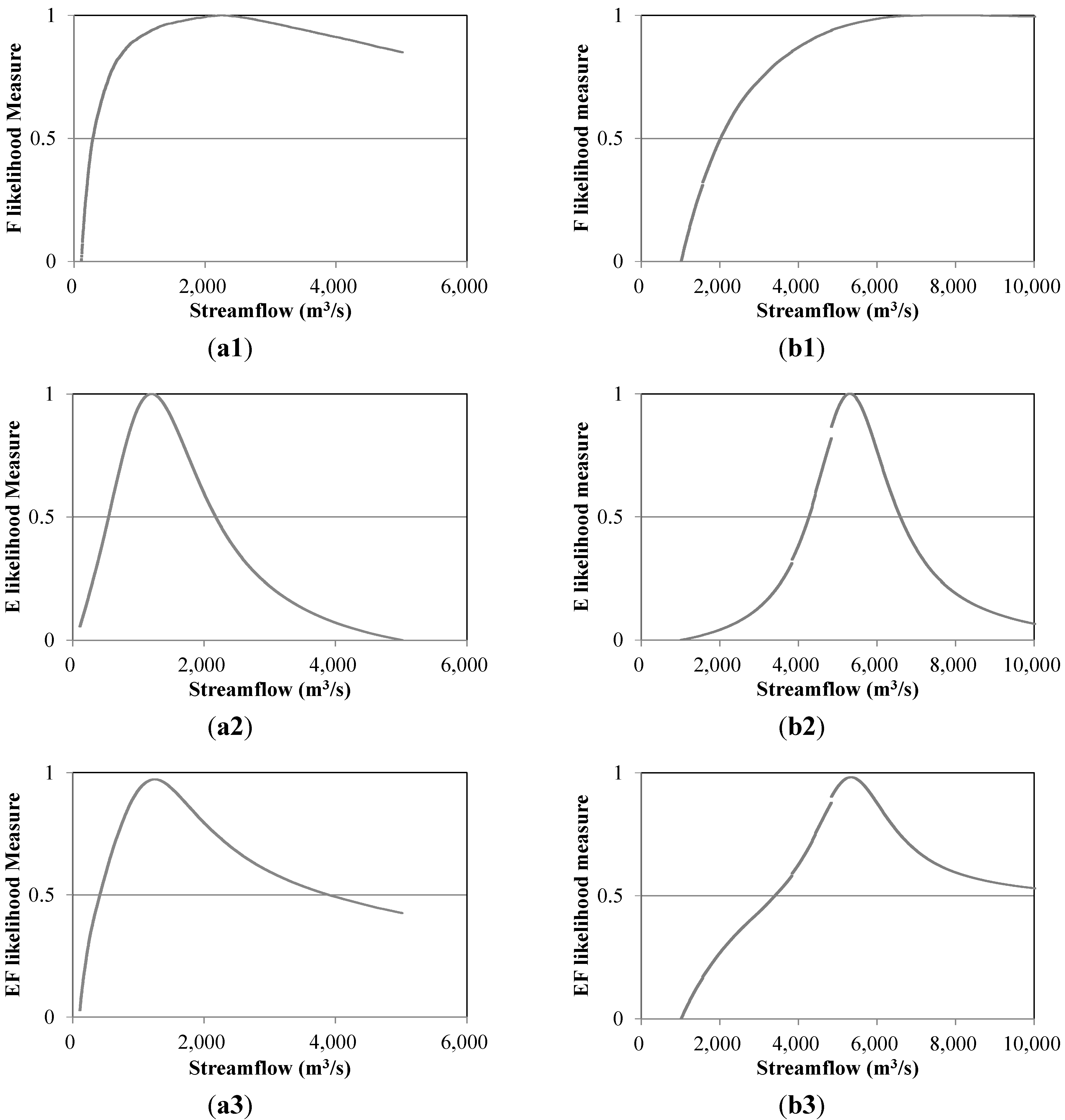
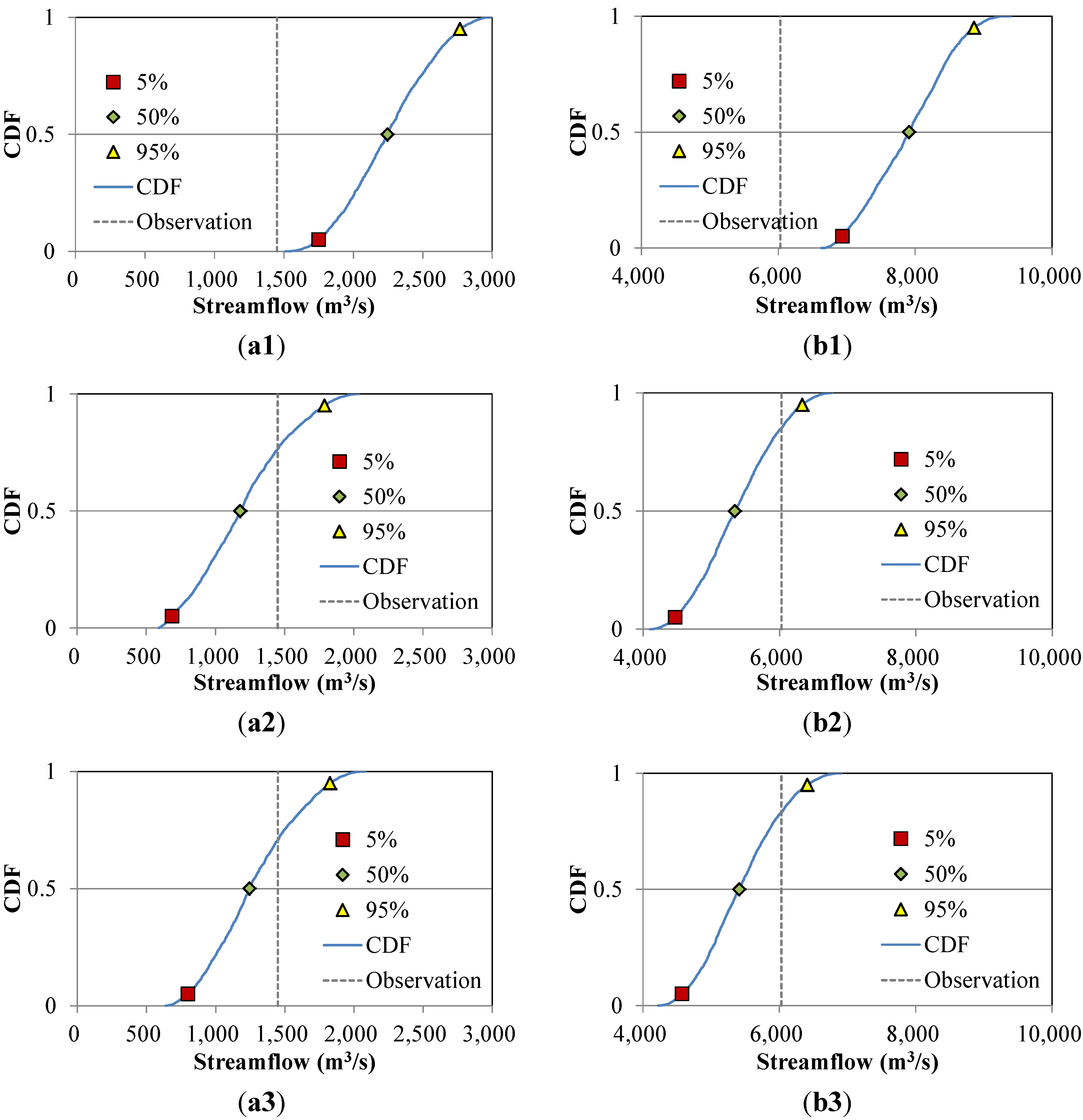
4.2. Approximation of Flood Discharge Using HEC-RAS and the GLUE Methodology

Results from Monte Carlo simulations for river discharge are presented in Figure 5. Results show that the water surface elevations obtained using satellite Landsat image and DEM for each study reach, are contained within boundaries of minimum and maximum outputs, based on a total of 10,000 simulations carried out by randomly sampling the steady discharge from the identified variation range and assuming a uniform probability distribution. The simulated water surface elevations over all cross-sections range from 143.26 m to 149.28 m for the Montezuma reach, and from 276.52 m to 281.86 m for the Nebraska reach, respectively. The simulation for the Nebraska reach is conducted with a wider range of discharge than that of the Montezuma reach, but results in a smaller deviation of the simulated water surface elevations. These surface elevations obtained from each simulation are used to calculate E likelihood measures [Equation (5)]. Water surface elevations produced from HEC-RAS are used to produce flood inundation areas using IDW interpolation. The minimum and maximum areas are 7.2 km2 and 16.8 km2 for the Montezuma reach, and 63.9 km2 and 144.1 km2 for the Nebraska reach, respectively. The Nebraska reach has a twice-longer river than the Montezuma reach. However, although minimum random discharge (1000 m3/s) in the Nebraska reach is much less than maximum (5000 m3/s) in the Montezuma reach, the minimum inundated area (63.9 km2) of the Nebraska reach is about four times larger than the maximum (16.8 km2) of the Montezuma reach. From these results, it can be expected that the flood inundation depth in the Nebraska reach is shallower than that in the Montezuma reach.
This study used NED DEMs with 10 m resolution for estimation of flood discharge, but available DEMs in most ungauged basins all over the world have low resolutions. Therefore, application using satellite-based DEMs such as SRTM, ASTER can enhance the value of the suggested methodology in ungauged basins for flood discharge estimation. In this context, Sanders [71] evaluated the effect of on-line DEMs such as NED (3 m, 10 m, and 30 m), SRTM (1 s and 3 s), IfSAR (3 m), and LiDAR (3 m) for flood inundation modeling, and obtained the result that the 3 s SRTM (90 m) produced a flood zone only 12% larger than NED DEMs (3 m, 10 m, and 30 m) predictions in the unsteady flow, and a 25% larger flood zone in the steady flow. In addition, the effect of DEM on flood inundation maps could further decrease when the discharge is high or inundated area is large. Thus, the topographic details extracted from high resolution DEM can over-estimate or under-estimate floodwater [72]. These results support the applicability of other satellite-based DEMs in the suggested methodology for flood inundation. However, it should be noted that this methodology has limitations corresponding to the uncertainty sources such as assumption of flow condition and the use of normal roughness values. If errors in the roughness value and flow condition are added, the range of the estimated discharge will be much wider due to uncertainty propagated from them. The assumption of flow condition that the main river and the floodplains can be simulated as a single channel leads to no storage effects in flood inundation modeling. Although the assumption is applied to the flood inundation modeling using hydraulic models [73,74,75], it still has a weakness that the simulated water levels using 1D hydraulic model can be overestimated or underestimated because the stored water in floodplain is not considered. In addition, the roughness is a key uncertainty source in flood inundation modeling. In particular, the HEC-RAS model is based on the Manning’s equation [Equation (2)], in which roughness is one of variables. In this study, normal roughness values [34] are used because calibration of the roughness is difficult without the observed discharge. However, we can expect that lower roughness will typically produce lower water level by Manning’s equation. In addition, there are additional uncertainty sources such as DEM, rating curve, modeling type, model set-up and assumption, model parameter, and lack of model calibration data in flood inundation modeling [76,77].
The results from Figure 6 show the PDF based on the rescaled likelihood measures of discharge based on three different likelihood functions (F, E, and EF) through the MC simulations. The rescaled value indicates the probability of discharge weighted by each likelihood measure.
Figure 6. PDFs of discharge based on the rescaled likelihood measure. F likelihood measure: (a1) Montezuma Reach; (b1) Nebraska Reach; E likelihood measure: (a2) Montezuma Reach; (b2) Nebraska Reach; The combination of E and F likelihood measure (EF likelihood measure): (a3) Montezuma Reach; (b3) Nebraska Reach.
Water 05 01598 g006
For both reaches, the distribution of F likelihood measure, considering only spatial distribution of flood extents, commonly show that they slope very steeply upwards in low discharge and very mildly downward (or almost constant) in high discharge (Figure 6a1,b1). This result is related to the shape of the valley in both study reaches. The U-shaped or rectangular valley has geometric characteristics where a variation of discharge leads to an abrupt change in the inundation area in low flow conditions and a slight change in high flow conditions. For E likelihood measure, considering only elevational differences, likelihood measures of discharge turn very steeply upwards in low discharge, and after the peak they turn very steeply downward in high discharge (Figure 6a2,b2). In this study, the peak in distribution of the E likelihood measure is obviously detected. The distribution of the likelihood measures is almost symmetrical for the Nebraska reach and positively skewed for the Montezuma reach. The distribution of the likelihood measures are likely to be skewed due to the side slope of the valley and the observed surface elevations. The EF likelihood measure of discharge are calculated by taking α of 0.5 in Equation (7), which is the average of F and E likelihood measures rescaled from 0 to 1. Figure 6a3,b3 shows that the PDFs of discharge based on EF likelihood measures follow the shape of the ones based on the E likelihood. In actual, α in EF likelihood measures can be another uncertainty source in the GLUE methodology. However, research about α will be performed in future because α is a factor to explain how physical characteristics of flood inundation affect to informal likelihood measure. For example, α in U-shaped valley will be greater than 0.5 for more accurate flood discharge approximation because the variation in discharge around fully filled water in the U-shaped valley brings very small change in flood inundation area.
Figure 7 and Table 4 show the results from GLUE that the boundaries of the approximated flood discharge is compared with the observations including water surface elevation and flood extents obtained from Landsat 5 TM imagery. The flood discharge is approximated on the CDFs of discharge, which are based on the behavioral models selected by taking the top 30% of each likelihood measure [52]. Figure 7 and Table 4 show the 5%, 50%, and 95% boundaries of the approximated flood discharge using different likelihood measures. The approximation boundary for the Nebraska reach is in the range of 6938 to 8862 m3/s for the F likelihood measure, 4471 to 6344 m3/s for the E likelihood, and 4576 to 6412 m3/s for the EF likelihood measure. The 50% of the CDF giving the deterministic model output, ranges from 5346 to 7911 m3/s. Considering the gauged discharge of 6030 m3/s, the relative errors of approximated discharge are in the range of 10% (617 m3/s) to 31% (−2830 m3/s). In the case of the Montezuma reach, the flood discharge over all likelihood measures is approximated in the range of 687 m3/s to 2769 m3/s. Considering the gauged discharge of 1450 m3/s, the relative errors range from 14% (205 m3/s) to 55% (−797 m3/s). From these results, E likelihood based on the elevational difference, commonly produced a much better approximation of discharge than the F likelihood measure, based on spatial differences for both study reaches. The use of the EF likelihood measure improves the approximation of discharge, by reducing the relative error of 1% for the Nebraska reach and 4% for the Montezuma reach. A relative error of 10% in the Nebraska reach indicates a better approximation of discharge than the 14% in the Montezuma reach. The gauged discharge used in this study is estimated from a stage-discharge rating curve involving uncertainty. For comparing results from the suggested method with uncertainty in rating curves, the regression equation for the stage-discharge rating curve based on peak flows provided by USGS is developed assuming a Student’s t-distribution (Figure 8). Using a 95% confidence interval, uncertainty for discharge of 1450 m3/s at USGS gauge station in Montezuma ranges from 938 to 2241 m3/s and uncertainty for discharge of 6030 m3/s at USGS gauge station in Nebraska city rages from 2263 to 16,048 m3/s. These results show that almost all discharge estimated by the suggested method are in the bound of uncertainty in discharge estimated from rating equations (Table 4). Figure 9 shows the simulated flood inundation maps for the approximated discharge, which are deterministic representation values (50% of CDF) based on the EF likelihood measure. Among the three different likelihood measures used in this study, EF likelihood measures commonly produced the best approximation of discharge for both study reaches.
Figure 7. Cumulative density function (CDF) obtained by taking top 30% of likelihood measure and the 5%, 50%, and 95% boundaries of the approximated flood discharge. Based on F likelihood measure: (a1) Montezuma Reach; (b1) Nebraska Reach; Based on E likelihood measure: (a2) Montezuma Reach; (b2) Nebraska Reach; Based on the combination of E and F likelihood measure (EF likelihood measure): (a3) Montezuma Reach: (b3) Nebraska Reach.
Water 05 01598 g007
Table 4. Boundaries of the approximated discharge for each likelihood measures.
Likelihood MeasureCDFDischarge (m3/s)
MontezumaNebraska
F0.0517526938
0.5022477911
0.9527698862
E0.056874471
0.5011795346
0.9517886344
EF0.058014576
0.5012455413
0.9518276412
Observation14506030
Figure 8. Stage-discharge rating curve based on peak flows provided by USGS. (a) Montezuma reach; (b) Nebraska reach.
Water 05 01598 g008
Figure 9. The simulated flood inundation maps for the approximated discharge (50% of CDF based on EF likelihood measure). (a) Montezuma (Q = 1245 m3/s); (b) Nebraska (Q = 5413 m3/s).
Water 05 01598 g009

5. Summary and Conclusions

Obtaining flood information in data-poor regions is a difficult and uncertain task, but is very valuable for flood risk management in order to protect human civilization and the environment. The development of GIS, launching devices, and optical sensors have helped to investigate and analyze spatiotemporal flood attributes for past flood events, and the use of remote sensing data can therefore supplement flood information in poorly gauged area. In this paper, we have demonstrated the potential of Landsat image and the GLUE methodology in obtaining hydro-information in an ungauged basin, where formal likelihood measures are unavailable. To demonstrate the approach suggested in this study, Landsat images and the GLUE methodology are used to approximate the flood discharge without information from the gauge stations, which existed in the area.
The following conclusions are drawn from this study:
  • This study demonstrates that Landsat imagery can be used as secondary source for discharge estimation in a data-poor environment. The water-body extracted from the Landsat imagery can be used in conjunction with a hydraulic model to estimate flood discharge. However, the use of Landsat imagery in a small-scale study can produce relatively more uncertainty in reading water surface elevation from a DEM (10 m × 10 m) than in a large-scale study, due to the coarse resolution (30 m × 30 m) of a Landsat image. Therefore, flood information obtained from Landsat imagery in planning flood risk management in a data-poor environment is more appropriate for larger rivers. The approximated flood discharge estimated for the Nebraska reach is 5413 m3/s, and 1245 m3/s for the Montezuma reach. The relative errors between the gauged data and the approximations are 10% for the Nebraska reach and 14% for the Montezuma reach, respectively.
  • In the GLUE methodology, the different results between E Likelihood measure and F likelihood measure showed subjectivity on the selection of criteria meeting informal likelihood measure. However, when considering the physical conditions of the study reach, such as the shape of the valley, size of the reach, and the flood intensity, the informal likelihood measure in the GLUE methodology can enhance the ability of finding improved flood information in data-poor environment. In addition, each likelihood measure is differently responded corresponding to the random discharge, but produces common results in flood discharge estimation for both study reaches. For example, the approximated discharge for both reaches is overestimated for F likelihood measure on the spatial flood extent and underestimated for E likelihood measure on the observed water surface elevation. In addition, the combination (EF likelihood) of two likelihood measures estimates discharge closest to the observed discharge at gauge station.
This study shows that the use of satellite imagery provides an economical way of obtaining flood information at a planning level in ungauged basins. The approach suggested in this study uses relatively high quality DEM in flood discharge approximation at only two study reaches. Therefore, application of this methodology using available DEMs, such as STRM and ASTER, in most ungauged areas all over the world would give a significant contribution to the applicability of the suggested method. In addition, understanding uncertainty source such as roughness and channel geometry will enhance the accuracy of flood damage estimation in ungauged basin. Moreover, Sufficient RS data with high quality for flood events will provide useful information such as the relationship between flood inundation area and flood level to flood risk management in ungauged basin [16,78]. In this regard, it needs the improvement in sensors and easy access in stationary satellites. Although the use of GLUE involves uncertainty in the subjective decisions on the selection of informal likelihood, the effect of the uncertainty can be reduced by combination of informal likelihood measures considering the surrounding conditions (e.g., EF likelihood measure). The approach suggested in this study is based on flood discharge approximation at only two study reaches. Therefore, more case studies with various physical conditions, higher dimensional hydraulic models, and different remote sensing data, would be helpful in generalizing the role of remote sensing data and GLUE in estimating flood discharge in data-poor environments.

Acknowledgments

This study was supported financially by the Construction Technology Innovation Program (08-Tech-Inovation-F01), through the Research Center of Flood Defense Technology for the Next Generation, at the Korea Institute of Construction & Transportation Technology Evaluation and Planning (KICTEP), in the Ministry of Land, Transport and Maritime Affairs (MLTM).

Conflicts of Interest

The authors declare no conflict of interest.

References

  1. Stedinger, J.R.; Vogel, R.M. Foufoula-Georgiou E. Frequency Analysis of Extreme Events. In Handbook of Hydrology; Maidment, D.R., Ed.; McGraw-Hill: New York, NY, USA, 1993. [Google Scholar]
  2. Ramachandra, R.A.; Hamed, K.H. Flood Frequency Analysis; CRC Press: Boca Raton, FL, USA, 2000; p. 350. [Google Scholar]
  3. Vogel, R.M.; McMahon, T.A.; Chiew, F. Floodflow frequency model selection in Australia. J. Hydrol. 1993, 146, 421–449. [Google Scholar] [CrossRef]
  4. Klemeš, V. Tall tales about tails of hydrological distributions. J. Hydrol. Engrg. ASCE 2003, 5, 232–239. [Google Scholar] [CrossRef]
  5. Mitosek, H.T.; Strupczewski, W.G.; Singh, V.P. Three procedures for selection of annual flood peak distribution. J. Hydrol. 2006, 323, 57–73. [Google Scholar] [CrossRef]
  6. Laio, F.; di Baldassarre, G.; Montanari, A. Model selection techniques for the frequency analysis of hydrological extremes. Water Resour. Res. 2009, 45, W07416. [Google Scholar] [CrossRef]
  7. Dalrymple, T. Flood Frequency Analyses; USGS Water Supply Paper 1543-A; USGS: Reston, VA, USA, 1960. [Google Scholar]
  8. Viviroli, D.; Zappa, M.; Schwanbeck, J.; Gurtz, J.; Weingartner, R. Continuous simulation for flood estimation in ungauged mesoscale catchments of Switzerland—Part I: Modelling framework and calibration results. J. Hydrol. 2009, 377, 191–207. [Google Scholar] [CrossRef]
  9. Viviroli, D.; Mittelbach, H.; Gurtz, J.; Weingartner, R. Continuous simulation for flood estimation in ungauged mesoscale catchments of Switzerland—Part II: Parameter regionalisation and flood estimation results. J. Hydrol. 2009, 377, 208–225. [Google Scholar] [CrossRef]
  10. Grimaldi, S.; Petroselli, A.; Serinaldi, F. Design hydrograph estimation in small and ungauged watersheds: Continuous simulation method versus event-based approach. Hydrol. Process. 2012, 26, 3124–3134. [Google Scholar] [CrossRef]
  11. Chow, V.T.; Maidment, D.R.; Mays, L.W. Applied Hydrology; McGraw-Hill: New York, NY, USA, 1988. [Google Scholar]
  12. Oberstadler, R.; Honsch, H.; Huth, D. Assessment of the mapping capabilities of ERS-1 SAR data for flood mapping: A case study of Germany. Hydrol. Process. 1997, 10, 1415–1425. [Google Scholar] [CrossRef]
  13. Sivapalan, M.; Takeuchi, K.; Franks, S.W.; Gupta, V.K.; Karambiri, H.; Lakshim, V.; Liang, X.; McDonnell, J.J.; Mendiondo, E.M.; Connell, O.; et al. IAHS decade on predictions in ungauged basins (PUB), 2003–2012: Shaping an exciting future for the hydrological sciences. Hydrol. Sci. J. 2003, 48, 857–880. [Google Scholar] [CrossRef]
  14. Montanari, M.; Hostache, R.; Matgen, P.; Schumann, G.; Pfister, L.; Hoffmann, L. Calibration and sequential updating of a coupled hydrologic–hydraulic model using remote sensing-derived water stages. Hydrol. Earth Syst. Sci. 2009, 13, 367–380. [Google Scholar] [CrossRef]
  15. Smith, L.C. Satellite remote sensing of river inundation area, stage and discharge: A review. Hydrol. Process. 1997, 11, 1427–1439. [Google Scholar] [CrossRef]
  16. Pan, F.; Nichols, J. Remote sensing of river stage using the cross sectional inundation area—River stage relationship (IARSR) constructed from digital elevation model data. Hydrol. Process. 2012. [Google Scholar] [CrossRef]
  17. Bates, P.D.; Horritt, M.S.; Smith, C.N.; Mason, D. Integrating remote sensing observations of flood hydrology and hydraulic modelling. Hydrol. Process. 1997, 11, 1777–1796. [Google Scholar] [CrossRef]
  18. Sun, W.C.; Ishidaira, W.H.; Bastola, S. Prospects for calibrating rainfall-runoff models using satellite observations of river hydraulic variables as surrogates for in situ river discharge measurements. Hydrol. Process. 2012, 26, 872–882. [Google Scholar] [CrossRef]
  19. Bjerklie, D.M.; Moller, D.; Smith, L.C.; Dingman, S.L. Estimating discharge in rivers using remotely sensed hydraulic information. J. Hydrol. 2005, 309, 191–209. [Google Scholar] [CrossRef]
  20. Getirana, A.C.V.; Peters-Lidard, C. Estimating water discharge from large radar altimetry datasets. Hydrol. Earth Sys. Sci. 2013, 17, 923–933. [Google Scholar] [CrossRef]
  21. Durand, M.; Andreadis, K.M.; Alsdorf, D.E.; Lettenmaier, D.P.; Moller, D.; Wilson, M. Estimation of bathymetric depth and slope from data assimilation of swath altimetry into a hydrodynamic model. Geophys. Res. Letters 2008, 35, L20401. [Google Scholar] [CrossRef]
  22. Neal, J.; Schumann, G.; Bates, P.; Buytaert, W.; Matgen, P.; Pappenberger, F. A data assimilation approach to discharge estimation from space. Hydrol. Process. 2009, 23, 3641–3649. [Google Scholar] [CrossRef]
  23. Hostache, R.; Lai, X.; Monnier, J.; Puech, C. Assimilation of spatially distributed water levels into a shallow-water flood model. Part II: Use of a remote sensing image of Mosel river. J. Hydrol. 2010, 390, 257–268. [Google Scholar] [CrossRef] [Green Version]
  24. Matgen, P.; Montanari, M.; Hostache, R.; Pfister, L.; Hoffmann, L.; Plaza, D.; Pauwels, V.R.N.; de Lannoy, G.J.M.; de Keyser, R.; Savenije, H.H.G. Towards the sequential assimilation of SAR-derived water stages into hydraulic models using the particle filter: Proof of concept. Hydrol. Earth Syst. Sci. 2010, 14, 1773–1785. [Google Scholar] [CrossRef] [Green Version]
  25. Beven, K.J.; Binley, A.M. The future of distributed models: Model calibration and uncertainty prediction. Hydrol. Process. 1992, 6, 279–298. [Google Scholar] [CrossRef]
  26. Romanowicz, R.; Beven, K.J. Dynamic real-time prediction of flood inundation probabilities. Hydrol. Sci. J. 1998, 43, 181–196. [Google Scholar] [CrossRef]
  27. Pappenberger, F.; Beven, K.J.; Hunter, N.M.; Bates, P.D.; Gouweleeuw, B.T.; Thielen, J.; de Roo, A.P.J. Cascading model uncertainty from medium range weather forecasts (10 days) through a rainfall-runoff model to flood inundation predictions within the European Flood Forecasting System (EFFS). Hydrol. Earth Syst. Sci. 2005, 9, 381–393. [Google Scholar] [CrossRef]
  28. Pappenberger, F.; Matgen, P.; Beven, K.; Henry, J.; Pfister, L.; de Fraipont, P. Influence of uncertain boundary conditions and model structure on flood inundation predictions. Adv. Water Resour. 2006, 29, 1430–1449. [Google Scholar] [CrossRef]
  29. Mantovan, P.; Todini, E. Hydrological forecasting uncertainty assessment: Incoherence of the GLUE methodology. J. Hydrol. 2006, 330, 368–381. [Google Scholar] [CrossRef]
  30. Beven, K.J.; Smith, P.J.; Freer, J.E. Comment on “Hydrological forecasting uncertainty assessment: Incoherence of the GLUE methodology” by Pietro Mantovan and Ezio Todini. J. Hydrol. 2007, 338, 315–318. [Google Scholar] [CrossRef]
  31. Beven, K.J.; Smith, P.J.; Freer, J.E. So just why would a modeller choose to be incoherent? J. Hydrol. 2008, 354, 15–32. [Google Scholar] [CrossRef]
  32. USGS Landsat Missions Home Page. Available online: http://landsat.usgs.gov/ (accessed on 26 September 2013).
  33. The National Map Viewer and Download Platform. Available online: http://seamless.usgs.gov/ (accessed on 26 September 2013).
  34. Moore, M.R. Development of a High-Resolution 1D/2D Coupled Flood Simulation of Charles City, Iowa. Master’s thesis, University of Iowa, Iowa city, IA, USA, May 2011. [Google Scholar]
  35. Chow, V.T. Open-Channel Hydraulics; McGraw-Hill: New York, NY, USA, 1959. [Google Scholar]
  36. Calenda, G.C.; Mancini, C.P.; Volpi, E. Distribution of extreme peak floods of the Tiber River from the XV century. Adv. Water Resour. 2005, 28, 615–625. [Google Scholar] [CrossRef]
  37. National Water Information System: Web Interface. USGS Water Resources. USGS 03340500. Available online: http://waterdata.usgs.gov/usa/nwis/uv?03340500 (accessed on 26 September 2013).
  38. National Water Information System: Web Interface. USGS Water Resources. USGS 06807000. Available online: http://waterdata.usgs.gov/usa/nwis/uv?site_no=06807000 (accessed on 26 September 2013).
  39. Tou, J.T.; Gonzales, R.C. Pattern Recognition Principles. Isodata Algorithm, Pattern Classification by Distance Functions; Addison-Wesley: Reading, MA, USA, 1974; pp. 97–104. [Google Scholar]
  40. Richards, J.A. Remote Sensing Digital Image Analysis: An Introduction, 2nd ed.; Springer-Verlag: Berlin, Germany, 1993. [Google Scholar]
  41. Castañeda, C.; Herrero, J.; Casterad, M.A. Facies identification within the playalakes of the Monegros Desert, Spain, with field and satellite data. Catena 2005, 63, 39–63. [Google Scholar] [CrossRef]
  42. Lang, M.W.; McCarty, G.W. LiDAR intensity for improved detection of inundation below the forest canopy. Wetlands 2009, 29, 1166–1178. [Google Scholar] [CrossRef]
  43. Thomas, N.E.; Huang, C.; Goward, S.N.; Powell, S.; Rishmawi, K.; Schleeweis, K.; Hinds, A. Validation of north American forest disturbance dynamics derived from Landsat time series stacks. Remote Sens. Environ. 2011, 115, 19–32. [Google Scholar] [CrossRef]
  44. Khan, S.I.; Hong, Y.; Wang, J.; Yilmaz, K.K.; Gourley, J.J.; Adler, R.F.; Brakenridge, G.R.; Policelli, F.; Habib, S.; Irwin, D. Satellite remote sensing and hydrologic modeling for flood inundation mapping in Lake Victoria basin: Implications for hydrologic prediction in ungauged basins. IEEE Trans. Geosci. Remote Sens. 2011, 49, 85–95. [Google Scholar] [CrossRef]
  45. Song, C.; Woodcock, C.E.; Seto, K.C.; Pax-Lenney, M.; Macomber, S.A. Classification and change detection using Landsat TM data: When and how to correct atmospheric effects. Remote Sens. Environ. 2001, 75, 230–244. [Google Scholar] [CrossRef]
  46. U.S. Army Corps of Engineers (USACE). HEC–RAS Hydraulic Reference Manual; Hydrologic Engineering Center: Davis, CA, USA, 2006. [Google Scholar]
  47. Pappenberger, F.; Beven, K.; Horritt, M.; Blazkova, S. Uncertainty in the calibration of effective roughness parameters in HEC-RAS using inundation and downstream level observations. J. Hydrol. 2005, 302, 46–69. [Google Scholar] [CrossRef]
  48. Horritt, M.S. A methodology for the validation of uncertain flood inundation models. J. Hydrol. 2006, 326, 153–165. [Google Scholar] [CrossRef]
  49. Fewtrell, T.J.; Bates, P.D.; Horritt, M.; Hunter, N.M. Evaluating the effect of scale in flood inundation modelling in urban environments. Hydrol. Process. 2008, 22, 5107–5118. [Google Scholar] [CrossRef]
  50. Hicks, F.E.; Peacock, T. Suitability of HEC-RAS for flood forecasting. Can. Water Resour. J. 2005, 30, 159–174. [Google Scholar] [CrossRef]
  51. Meselhe, E.A.; Pereira, J.F.; Georgiou, I.Y.; Allison, M.A.; McCorquodale, J.A.; Davis, M.A. Numerical Modeling of Mobile-Bed Hydrodynamics in the Lower Mississippi River. American Society of Civil Engineers. In Proceedings of the World Environmental and Water Resources Congress (EWRI), Providence, RI, USA, 16–20 May 2010; pp. 1433–1442.
  52. Hornberger, G.M.; Spear, R.C. An approach to the preliminary analysis of environmental systems. J. Environ. Manag. 1981, 12, 7–18. [Google Scholar]
  53. Young, P.C. The Validity and Credibility of Models for Badlydefined Systems. Uncertainty and Forecasting of Water Quality; van Straten, B., Ed.; Springer: Berlin, Germany, 1983; pp. 69–98. [Google Scholar]
  54. Beven, K.J. Environmental Modelling: An Uncertain Future? Routledge: London, UK, 2009. [Google Scholar]
  55. Wang, X.; Frankenberger, J.R.; Kladivko, E.J. Uncertainties in DRAINMOD predictions of subsurface drain flow for an Indiana silt loam using the GLUE methodology. Hydrol. Process. 2006, 20, 3069–3084. [Google Scholar] [CrossRef]
  56. Blasone, R.S.; Madsen, H.; Rosbjerg, D. Uncertainty assessment of integrated distributed hydrological models using GLUE with Markov chain Monte Carlo sampling. J. Hydrol. 2008, 353, 18–32. [Google Scholar] [CrossRef]
  57. Blasone, R.S.; Vrugt, J.A.; Madsen, H.; Rosbjerg, D.; Robinson, B.A.; Zyvoloski, G.A. Generalized likelihood uncertainty estimation (GLUE) using adaptive Markov chain Monte Carlo sampling. Adv. Water Resour. 2008, 31, 630–648. [Google Scholar] [CrossRef]
  58. Hornberger, G.M.; Cosby, B.J. Selection of parameter values in environmental models using sparse data: A case study. Appl. Math. Comp. 1985, 17, 335–355. [Google Scholar]
  59. Kiczko, A.; Pappenberger, F.; Romanowicz, R.J. Flood Risk Analysis of the Warsaw Reach of the Vistula River. In ERB 2006: Uncertainties in the ‘Monitoring-Conceptualisation-Modelling’ Sequence of Catchment Research; European Network of Experimental and Representative Basins (ERB): Luxembourg, 2007. [Google Scholar]
  60. Aronica, G.; Hankin, B.G.; Beven, K.J. Uncertainty and equifinality in calibrating distributed roughness coefficients in a flood propagation model with limited data. Adv. Water Resour. 1998, 22, 349–365. [Google Scholar] [CrossRef]
  61. Hunter, N.M.; Bates, P.D.; Horritt, M.S.; de Roo, A.P.T.; Werner, M.G.F. Utility of different data types for calibrating flood inundation models within a GLUE framework. Hydrol. Earth Syst. Sci. 2005, 9, 412–430. [Google Scholar] [CrossRef]
  62. Schumann, G.; Cutler, M.; Black, A.; Matgen, P.; Pfister, L.; Hoffmann, L.; Pappenberger, F. Evaluating uncertain flood inundation predictions with uncertain remotely sensed water stages. Int. J. River Basin Manag. 2008, 6, 187–199. [Google Scholar] [CrossRef]
  63. Horritt, M.S.; Bates, P.D. Evaluation of 1D and 2D numerical models for predicting river flood inundation. J. Hydrol. 2002, 268, 87–89. [Google Scholar] [CrossRef]
  64. Schumann, G.; Bates, P.D.; Horritt, M.S.; Matgen, P.; Pappenberger, F. Progress in integration of remote sensing derived flood extent and stage data and hydraulic models. Rev. Geophys. 2009, 47. [Google Scholar] [CrossRef]
  65. Di Baldassarre, G.; Schumann, G.; Bates, P.D. A technique for the calibration of hydraulic models using uncertain satellite observations of flood extent. J. Hydrol. 2009, 367, 276–282. [Google Scholar] [CrossRef]
  66. Horritt, M.S.; Bates, P.D. Predicting floodplain inundation: Raster-based modelling versus the finite element approach. Hydrol. Process. 2001, 15, 825–842. [Google Scholar] [CrossRef]
  67. Aronica, G.; Bates, P.D.; Horritt, M.S. Assessing the uncertainty in distributed model predictions using observed binary pattern information within GLUE. Hydrol. Process. 2002, 16, 2001–2016. [Google Scholar] [CrossRef]
  68. Bates, P.D.; Horritt, M.S.; Aronica, G.; Beven, K.J. Bayesian updating of flood inundation likelihoods conditioned on flood extent data. Hydrol. Process. 2004, 18, 3347–3370. [Google Scholar] [CrossRef]
  69. Pappenberger, F.; Frodsham, K.; Beven, K.J.; Romanowicz, R.; Matgen, P. Fuzzy set approach to calibrating distributed flood inundation models using remote sensing observation. Hydrol. Earth Syst. Sci. 2007, 11, 739–752. [Google Scholar] [CrossRef]
  70. Cook, A.; Merwade, V. Effect of topographic data, geometric configuration and modeling approach on flood inundation mapping. J. Hydrol. 2009, 377, 131–142. [Google Scholar] [CrossRef]
  71. Sanders, B.F. Evaluation of on-line DEMs for flood inundation modeling. Adv. Water Resour. 2007, 30, 1831–1843. [Google Scholar] [CrossRef]
  72. Zheng, T.; Wang, Y. Mapping flood extent using a simple DEM-inundation model. North Carol. Geographer. 2007, 15, 1–19. [Google Scholar]
  73. Bates, P.D.; Horritt, M.S.; Hunter, N.M.; Mason, D.C.; Cobby, D.M. Numerical Modelling of Floodplain Flow. In Computational Fluid Dynamics:Applications in Environmental Hydraulics; Bates, P., Ferguson, L., Eds.; John Wiley and Sons Ltd.: Chichester, UK, 2005. [Google Scholar]
  74. Fewtrell, T.J.; Neal, J.C.; Bates, P.D.; Harison, P.J. Geometric and structural river channel complexity and the prediction of urban inundation. Hydrol. Process. 2011, 25, 3173–3186. [Google Scholar] [CrossRef]
  75. Jung, Y.; Merwade, V. Uncertainty quantification in flood inundation mapping using generalized likelihood uncertainty estimate and sensitivity analysis. J. Hydrol. Eng. 2012, 17, 507–520. [Google Scholar] [CrossRef]
  76. Bales, J.D.; Wagner, C.R. Sources of uncertainty in flood inundation maps. J Flood Risk Manag. 2009, 2, 139–147. [Google Scholar] [CrossRef]
  77. Merwade, V.M.; Olivera, F.; Arabi, M.; Edleman, S. Uncertainty in flood inundation mapping—Current issues and future directions. ASCE J. Hydrol. Eng. 2008, 13, 608–620. [Google Scholar] [CrossRef]
  78. Pan, F.; Liao, J.; Li, X.; Guo, H. Application of the inundation area-lake level rating curves constructed from the SRTM DEM to retrieving lake levels from satellite measured inundation areas. Comput. Geosci. 2013, 52, 168–176. [Google Scholar] [CrossRef]

