Impacts of Future Climate Change and Baltic Sea Level Rise on Groundwater Recharge, Groundwater Levels, and Surface Leakage in the Hanko Aquifer in Southern Finland

Abstract
:
1. Introduction
2. Materials
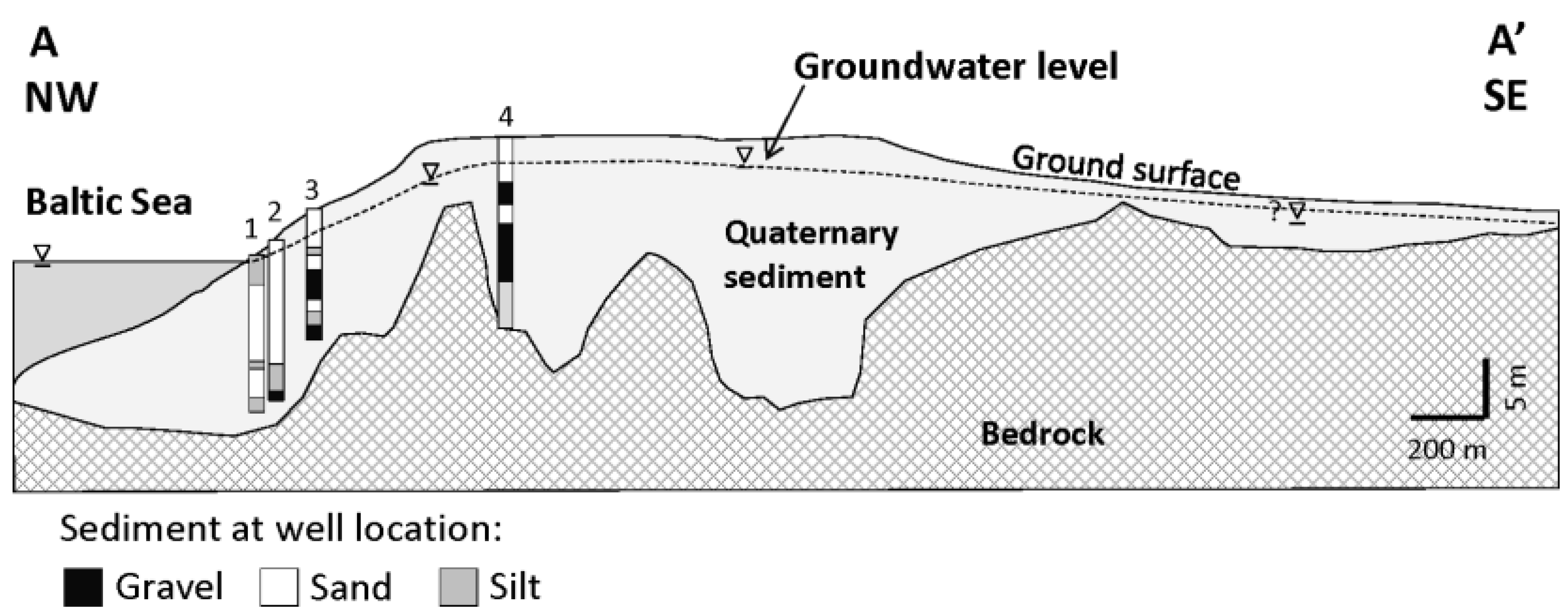
2.1. Study Area


2.2. Groundwater Level Data
2.3. Climate Data and Climate Change Scenarios
2.4. Sea Level Data and Sea Level Rise Scenarios

3. Methods
3.1. The Snow and Potential Evapotranspiration (PET) Models
3.2. Model Calibrations for the Snow and PET Models

3.3. Unsaturated Flow (UZF1 Package)

| Name | Description | Value Used in the Model |
|---|---|---|
| FINF | Potential Infiltration rate (m/d) | Estimated by the snowmelt model |
| PET | ET demand rate (m/d) | Estimated by the PET model |
| EXTDP | Extinction depth (m) | 0.5 |
| EXTWC | Extinction water content | 0.01 |
| EPS | Brook-Corey epsilon | 4.0 |
| THTS | Saturated water content | 0.3 |
| THTI | Initial water content | 0.2 |
| NUZTOP | Recharge/discharge location | Highest active cell |
| IUZFOPT | Unsaturated zone Kv (m/d) | Kv from the LPF package |
| VKS | Saturated zone Kv (m/d) | Kv from the LPF package |
| NTRAIL2 | Number of trailing waves | 10 |
| NSETS2 | Number of wave sets | 20 |
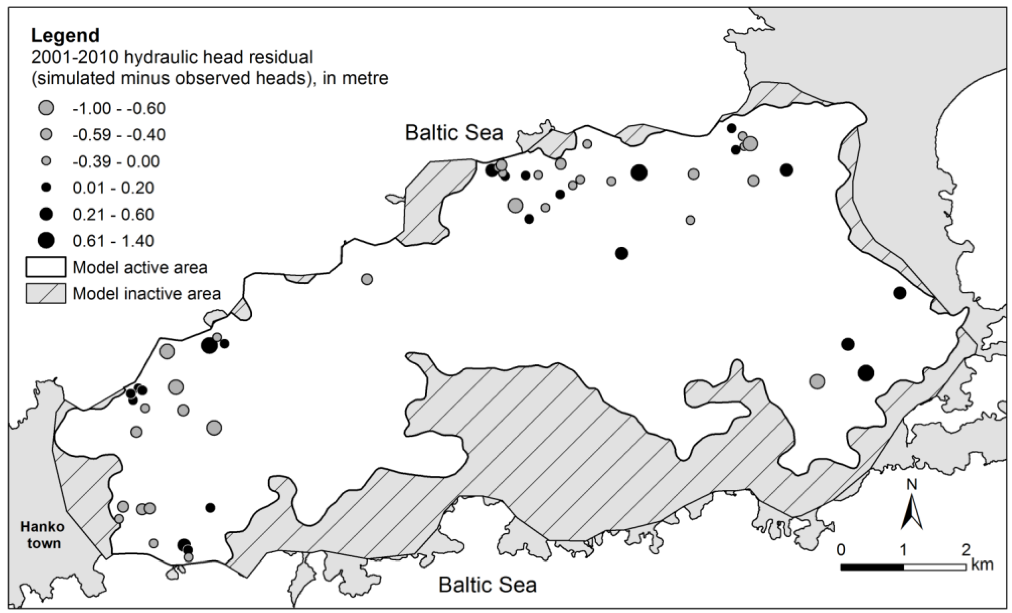
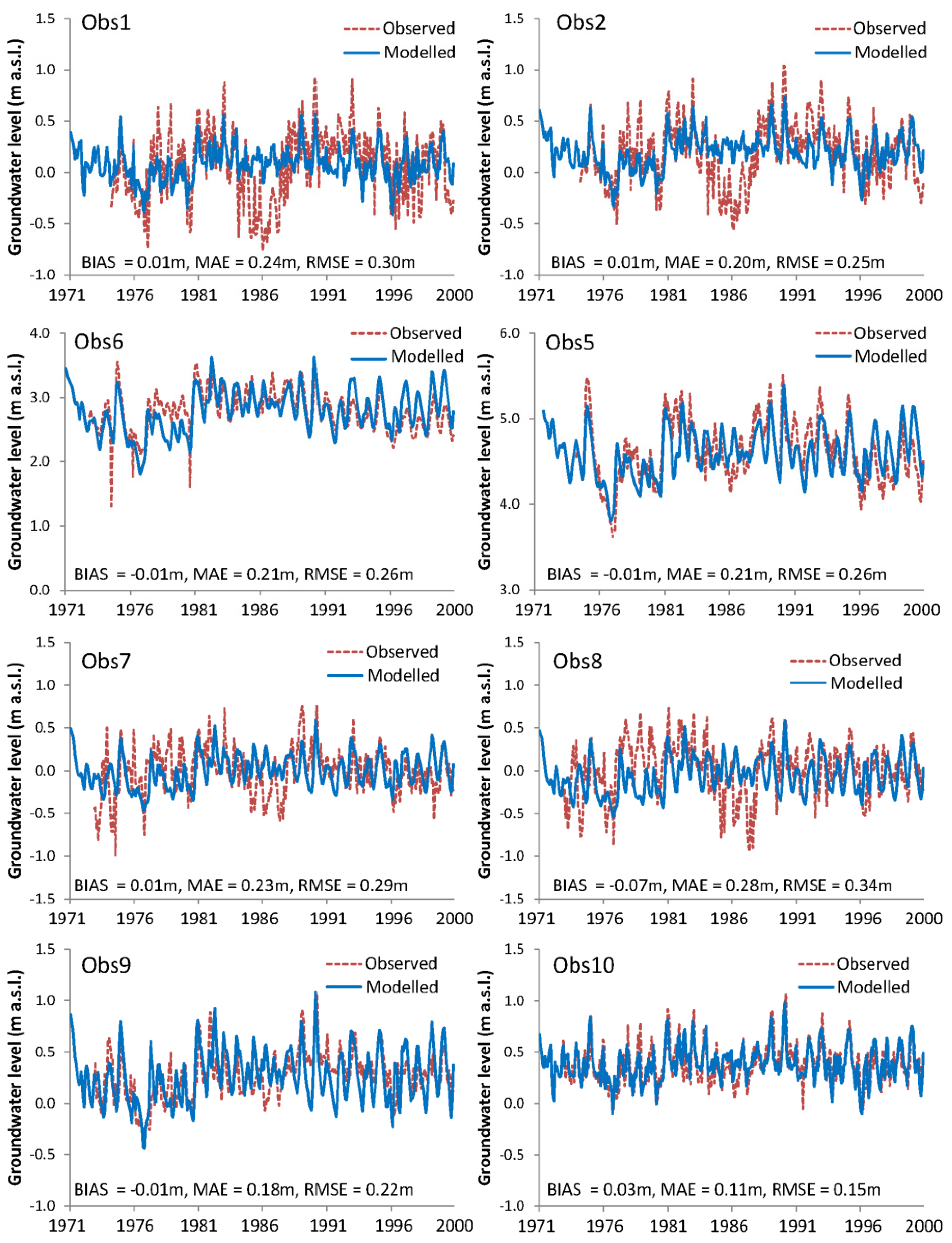
3.4. Groundwater Flow Model and Model Calibration


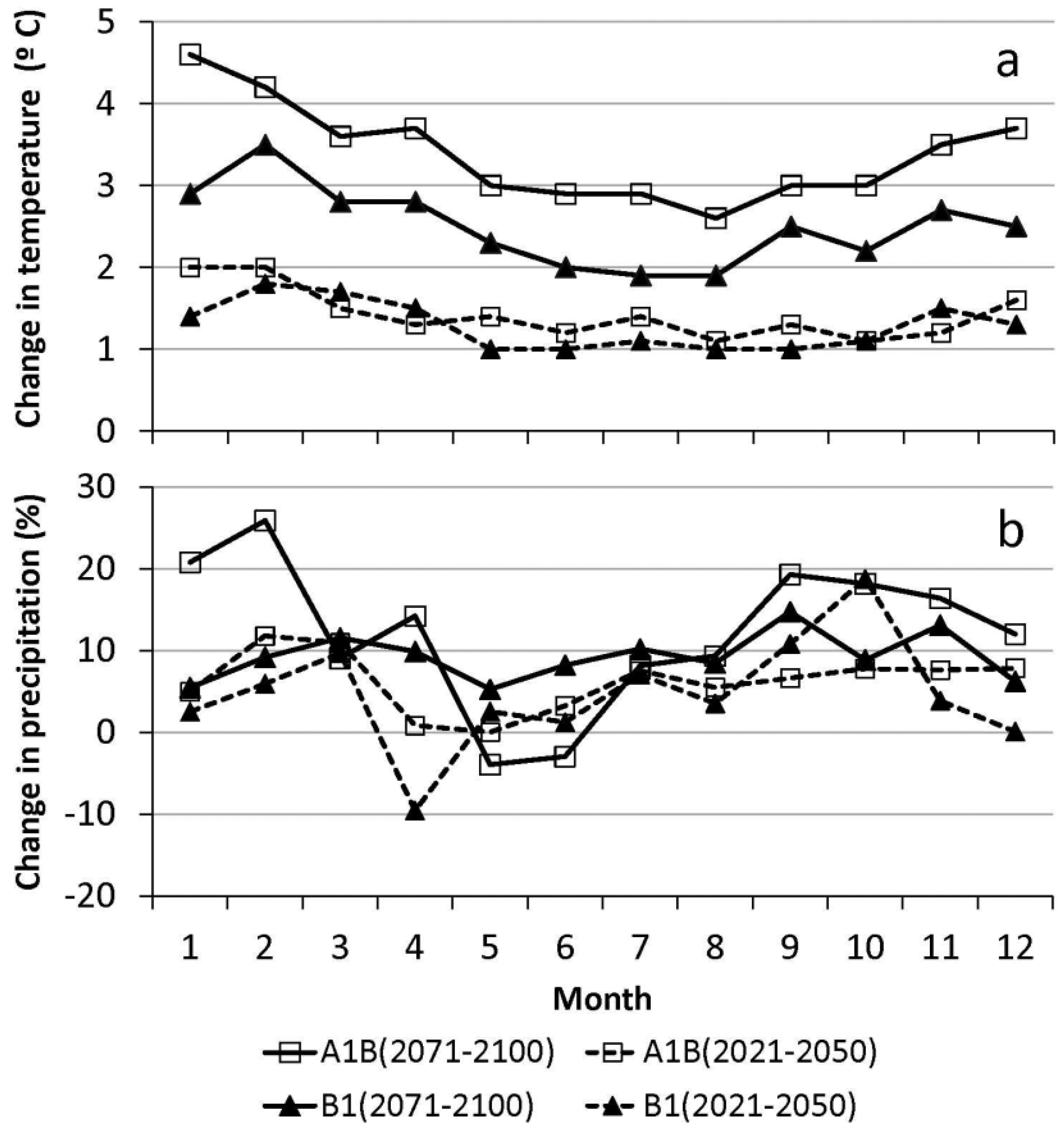
3.5. Climate Change Scenarios
4. Results
4.1. Climate Variables and Sea Level

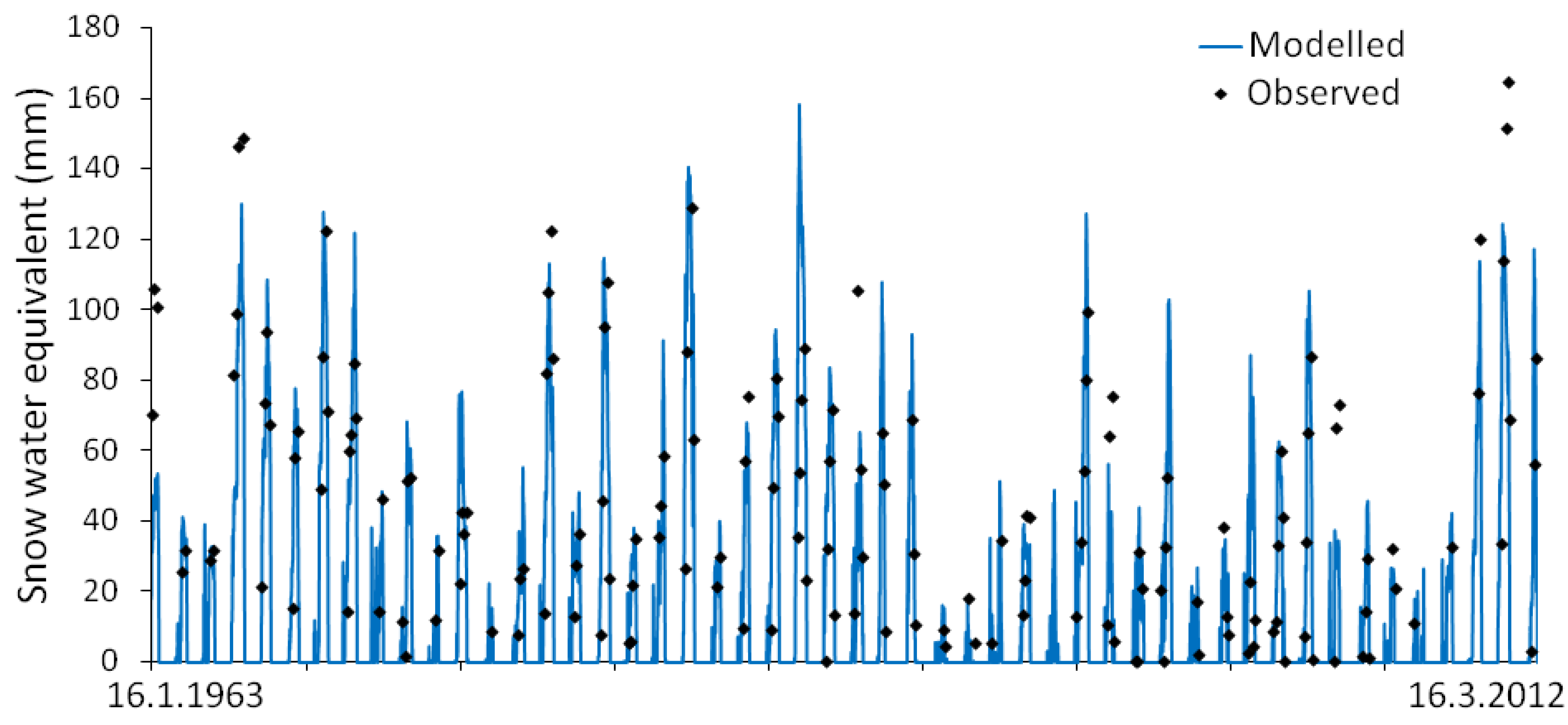
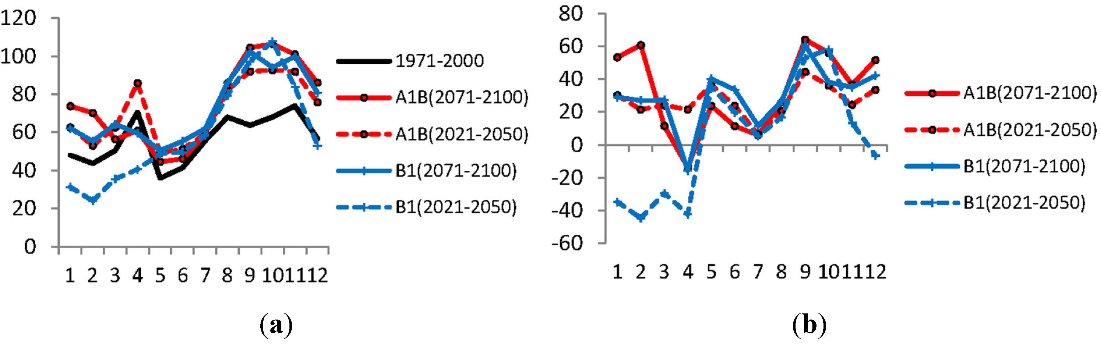
4.2. Snow-PET Model

| Month | 1971–2000 | A1B (2071–2100) | A1B (2021–2050) | B1 (2071–2100) | B1 (2021–2050) |
|---|---|---|---|---|---|
| January | 48 | 75 | 63 | 62 | 31 |
| February | 44 | 70 | 53 | 55 | 24 |
| March | 50 | 56 | 63 | 64 | 36 |
| April | 71 | 61 | 86 | 59 | 41 |
| May | 36 | 45 | 49 | 51 | 49 |
| June | 41 | 46 | 51 | 55 | 50 |
| July | 56 | 60 | 59 | 62 | 59 |
| August | 68 | 87 | 82 | 86 | 79 |
| September | 64 | 108 | 92 | 102 | 97 |
| October | 68 | 107 | 93 | 94 | 108 |
| November | 74 | 105 | 92 | 100 | 84 |
| December | 57 | 86 | 76 | 81 | 53 |
| Annual | 676 | 906 | 858 | 872 | 710 |
4.3. UZF1-MODFLOW
4.3.1. UZF1 Infiltration and UZF1 ET in the Unsaturated Zone

4.3.2. Evapotranspiration in the Saturated Zone (GW ET) and Groundwater Recharge
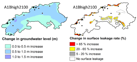
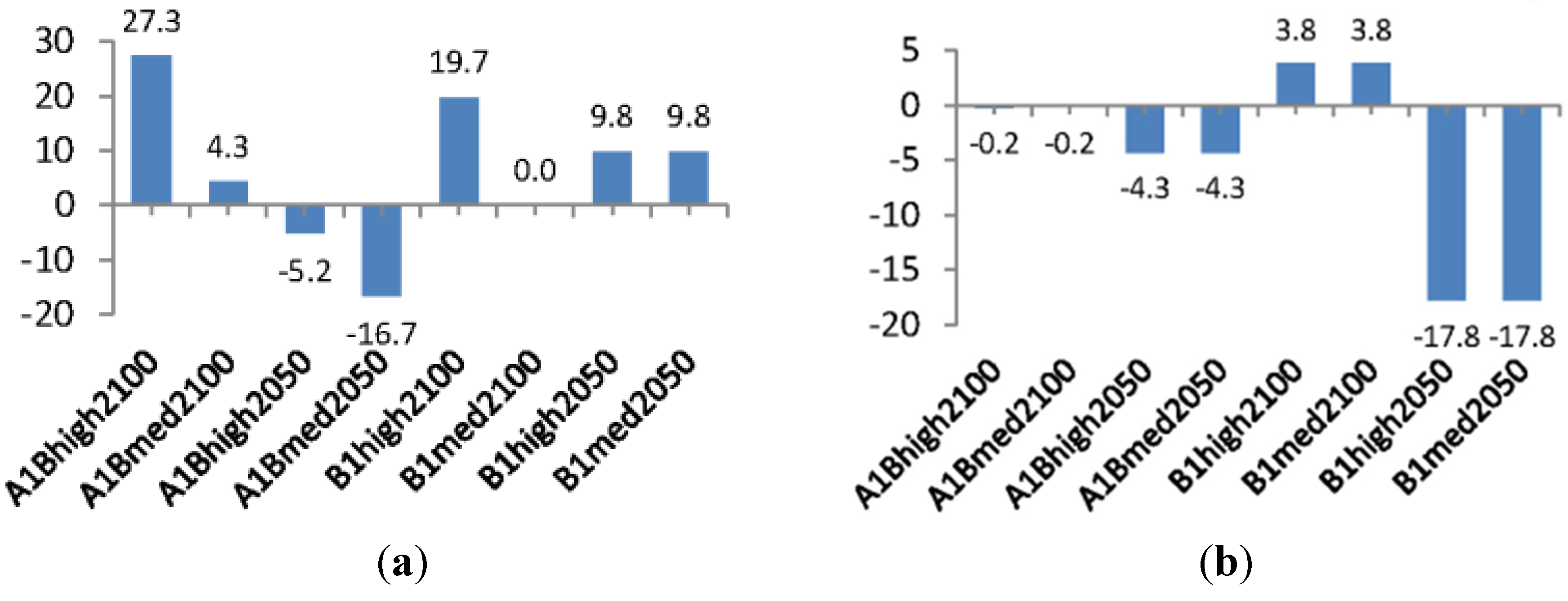
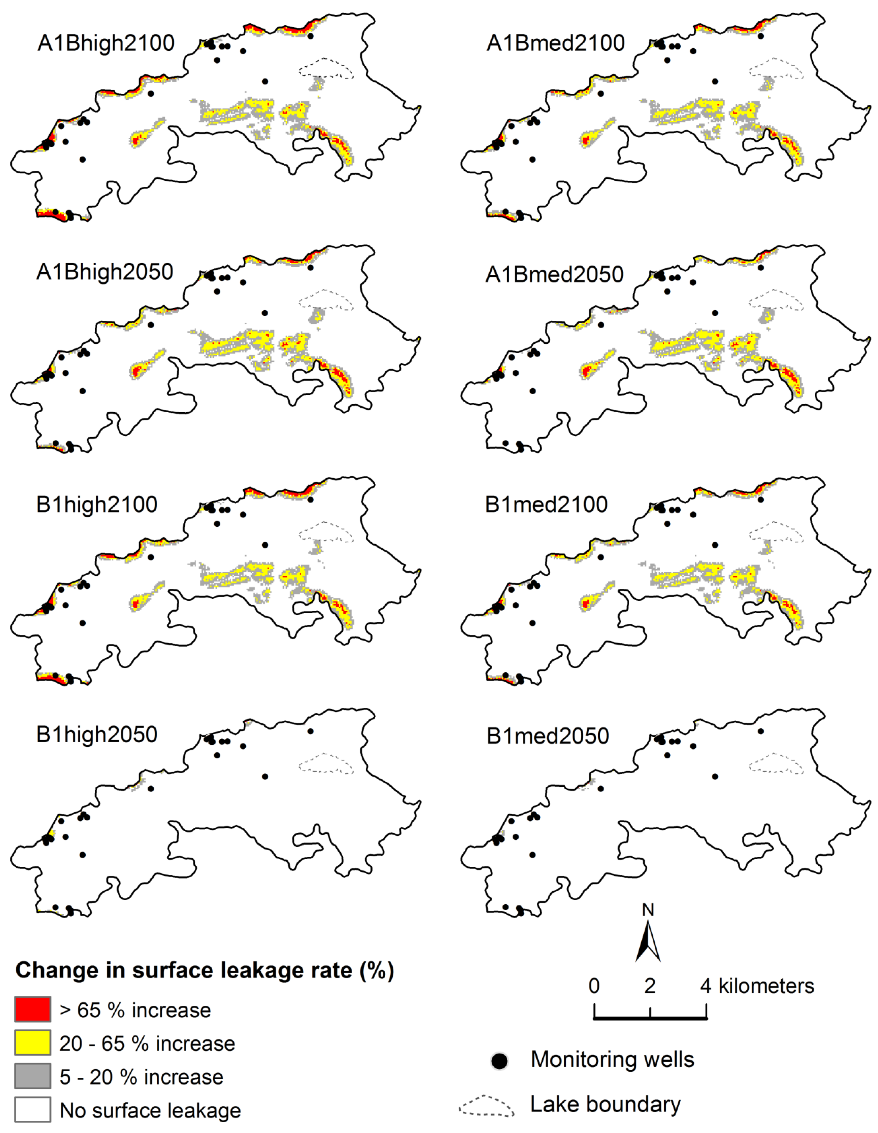
4.3.3. Surface Leakage
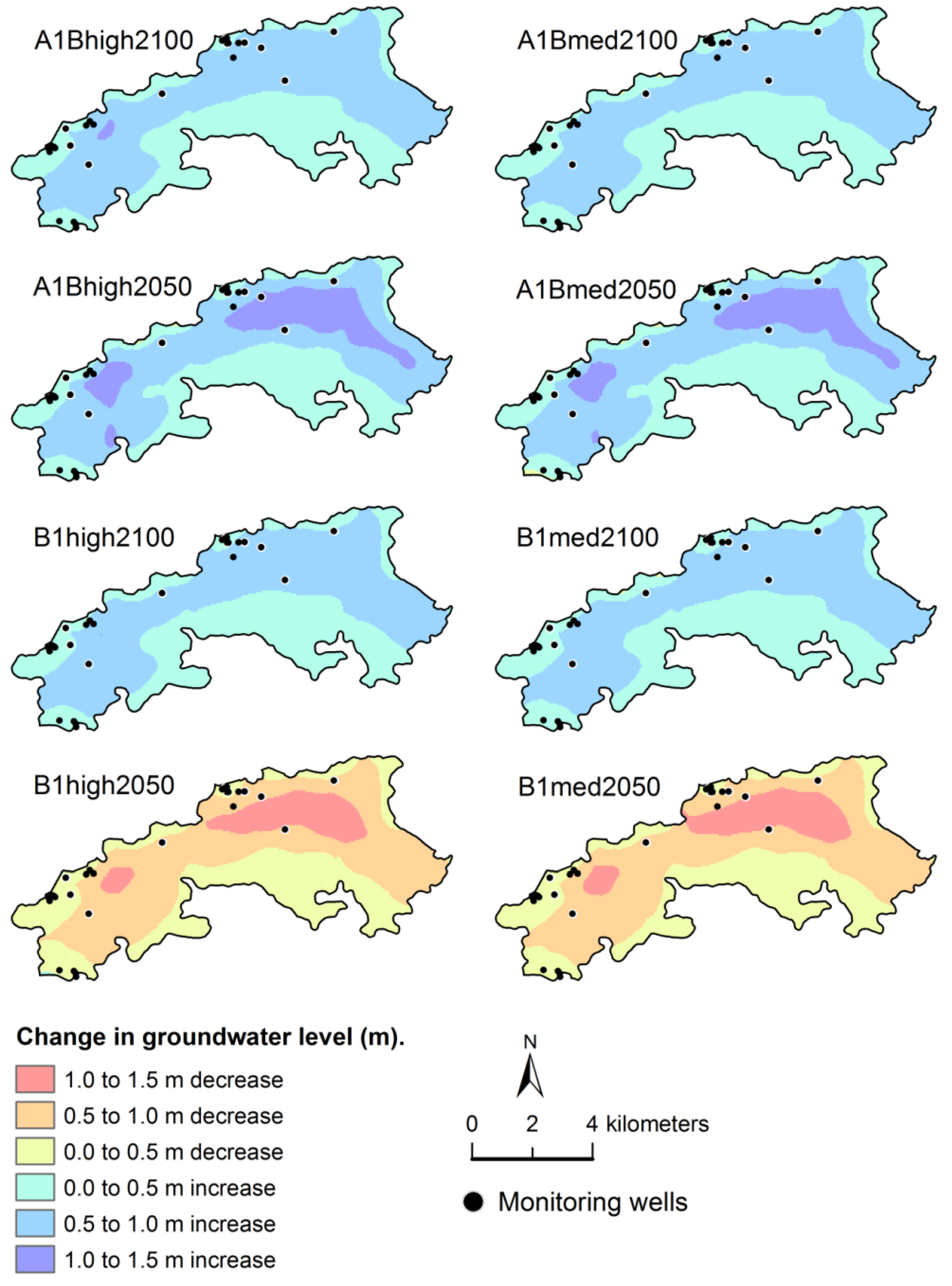
4.3.4. Relative Change in Groundwater Level and Baltic Sea Level

| Surface Leakage | Recharge | Inflow |
|---|---|---|
| A1Bhigh(2071–2100) | 0.55 | 0.55 |
| A1Bmed(2071–2100) | 0.67 | 0.41 |
| B1high(2071–2100) | 0.56 | 0.48 |
| B1med(2071–2100) | 0.62 | 0.37 |
| A1Bhigh(2021–2050) | 0.61 | 0.37 |
| A1Bmed(2021–2050) | 0.65 | 0.32 |
| B1high(2021–2050) | 0.35 | 0.67 |
| B1med(2021–2050) | 0.35 | 0.67 |

4.3.5. Change in Water Storage
4.4. Groundwater Level


5. Discussion
6. Conclusions
Acknowledgments
Conflicts of Interest
References
- Intergovernmental Panel on Climate Change. Emissions Scenarios: Summary for Policymakers—A Special Report of IPCC Working Group III. Available online: http://www.ipcc.ch/pdf/special-reports/spm/sres-en.pdf (accessed on 21 November 2011).
- Intergovernmental Panel on Climate Change. Climate Change 2007: Impacts, Adaptation and Vulnerability—Summary for Policymakers. In Contribution of Working Group II to the Fourth Assessment Report of the Intergovernmental Panel on Climate Change; Parry, M.L., Canziani, O.F., Palutikof, J.P., van der Linden, P.J., Hanson, C.E., Eds.; Cambridge University Press: Cambridge, UK, 2007; pp. 7–22. [Google Scholar]
- Oude Essink, G.H.P. Impact of sea-level rise in the Netherlands. In Seawater Intrusion in Coastal Aquifers: Concepts, Methods and Practices, Theory and Applications of Transport in Porous Media; Bear, J., Cheng, A.H.D., Sore, S., Quasar, D., Herrera, I., Eds.; Kluwer Academy: Norwell, MA, USA, 1999; pp. 507–530. [Google Scholar]
- Oude Essink, G.H.P. Improving fresh groundwater supply-problems and solutions. Ocean Coast. Manag. 2001, 44, 429–449. [Google Scholar]
- Oude Essink, G.H.P.; van Baaren, E.S.; de Louw, P.G.B. Effects of climate change on coastal groundwater systems: A modeling study in the Netherlands. Water Resour. Res. 2010, 46. [Google Scholar] [CrossRef]
- Rasmussen, P.; Sonnenborg, T.O.; Goncear, G.; Hinsby, K. Assessing impacts of climate change, sea level rise, and drainage canals on saltwater intrusion to coastal aquifer. Hydrol. Earth Syst. Sci. 2013, 17, 421–443. [Google Scholar] [CrossRef]
- Niswonger, R.G.; Prudic, D.E.; Regan, R.S. Documentation of the Unsaturated-Zone Flow (UZF1) Package for Modeling Unsaturated Flow between the Land Surface and the Water Table with MODFLOW-2005; U.S. Geological Survey Techniques and Methods 6-A19; U.S. Geological Survey: Reston, VA, USA, 2006; p. 62.
- Korkka-Niemi, K. Cumulative geological, regional and site-specific factors affecting groundwater quality in domestic wells in Finland. In Monographs of the Boreal Environment Research 20; Vammalan Kirjapaino Oy: Vammala, Finland, 2001; p. 100. [Google Scholar]
- Scibek, J.; Allen, D.M. Modeled Impacts of Predicted Climate Change on Recharge and Groundwater Levels. Water Resour. Res. 2006, 42. [Google Scholar] [CrossRef]
- Scibek, J.; Allen, D.M. Comparing the responses of two high permeability, unconfined aquifers to predicted climate change. Glob. Planet Chang. 2006, 50, 50–62. [Google Scholar] [CrossRef]
- Scibek, J.; Allen, D.M.; Cannon, A.; Whitfield, P. Groundwater-surface water interaction under scenarios of climate change using a high-resolution transient groundwater model. J. Hydrol. 2007, 333, 165–181. [Google Scholar] [CrossRef]
- Jyrkama, I.M.; Sykes, J.F. The impact of climate change on spatially varying groundwater recharge in the Grand River watershed (Ontario). J. Hydrol. 2007, 338, 237–250. [Google Scholar] [CrossRef]
- Okkonen, J. Groundwater and Its Response to Climate Variability and Change in Cold Snow Dominated Regions in Finland: Methods and Estimations. Ph.D. Thesis, Department of Process and Environmental Engineering, University of Oulu, Oulu, Finland, 2011. [Google Scholar]
- Jackson, C.R.; Meister, R.; Prudhomme, C. Modeling the effects of climate change and its uncertainty on UK Chalk groundwater resources from an ensemble of global climate model projections. J. Hydrol. 2011, 399, 12–28. [Google Scholar] [CrossRef] [Green Version]
- Ali, R.; McFarlane, D.; Varma, S.; Dawes, W.; Emelyanova, I.; Hodgson, G.; Charles, S. Potential climate change impacts on groundwater resources of south-western Australia. J. Hydrol. 2012, 475, 456–472. [Google Scholar] [CrossRef]
- Assefa, K.A.; Woodbury, A.D. Transient, spatially varied groundwater recharge modeling. Water Resour. Res. 2013, 49, 4593–4606. [Google Scholar] [CrossRef]
- Therrien, R.; McLaren, R.G.; Sudicky, E.A.; Park, Y.J. HydroGeoSphere—A Three-Dimensional Numerical Model Describing Fully-Integrated Subsurface and Surface Flow and Solute Transport; Groundwater Simulations Group, University of Waterloo: Waterloo, ON, Canada, 2012; p. 455. [Google Scholar]
- Kolditz, O.; Bauer, S.; Bilke, L.; Böttcher, N.; Delfs, J.O.; Fischer, T.; Görke, U.J.; Kalbacher, T.; Kosakowski, G.; McDermott, C.I.; et al. OpenGeoSys: An open source initiative for numerical simulation of thermo-hydro-mechanical/chemical (THM/C) processes in porous media. Environ. Earth Sci. 2012, 62, 589–599. [Google Scholar] [CrossRef]
- Maxwell, R.M.; Miller, N.L. Development of a coupled land surface and groundwater model. J. Hydrometeorol. 2005, 6, 233–247. [Google Scholar] [CrossRef]
- Kollet, S.J.; Maxwell, R.M. Capturing the influence of groundwater dynamics on land surface processes using an integrated, distributed watershed model. Water Resour. Res. 2008, 44. [Google Scholar] [CrossRef]
- Warsta, L. Modelling Water Flow and Soil Erosion in Clayey, Subsurface Drained Agricultural Fields. Ph.D. Thesis, Department of Civil and Environmental Engineering, Aalto University, Espoo, Finland, 2011. [Google Scholar]
- Harter, T.; Morel-Seytoux, H. Peer Review of the IWFM, MODFLOW and HGS Model Codes: Potential for Water Management Applications in California’s Central Valley and Other Irrigated Groundwater Basins-Final Report; California Water and Environmental Modeling Forum: Sacramento, CA, USA, August 2013. [Google Scholar]
- Niswonger, R.G.; Prudic, D.E. Modeling variably saturated flow using kinematic waves in MODFLOW. In Groundwater Recharge in a Desert Environment; Hogan, J.F., Phillips, F.M., Scanlon, B.R., Eds.; American Geophysical Union: Washington, DC, USA, 2004. [Google Scholar]
- Seo, H.S.; Šimůnek, J.; Poeter, E.P. Documentation of the HYDRUS package for MODFLOW-2000, the U.S. Geological Survey Modular Groundwater Model; GWMI 2007–01; International Ground Water Modeling Center, Colorado School of Mines: Golden, CO, USA, 2007. [Google Scholar]
- Harbaugh, A.W. MODFLOW-2005, the U.S. Geological Survey Modular Ground-Water Model—The Ground-Water Flow Process; U.S. Geological Survey Techniques and Methods 6-A16; U.S. Geological Survey: Reston, VA, USA, 2005; p. 253.
- Harbaugh, A.W.; Banta, E.R.; Hill, M.C.; McDonald, M.G. MODFLOW-2000, the U.S. Geological Survey Modular Ground-Water Model-Modularization Concepts and the Ground-Water Flow Process; U.S. Geological Survey Open-File Report 00-92; U.S. Geological Survey: Reston, VA, USA, 2000; p. 121.
- Twarakavi, N.K.C.; Šimůnek, J.; Seo, S. Evaluating interactions between groundwater and vadose zone using the HYDRUS-based flow package for MODFLOW. Vadose Zone J. 2008, 7, 757–768. [Google Scholar] [CrossRef]
- Twarakavi, N.K.C.; Šimůnek, J.; Seo, S. Reply to “Comment on ‘Evaluating Interactions between Groundwater and Vadose Zone Using the HYDRUS-based Flow Package for MODFLOW”. Vadose Zone J. 2009, 8, 820–821. [Google Scholar] [CrossRef]
- Niswonger, R.G.; Prudic, D.E. Comment on “Evaluating interactions between groundwater and vadose zone using the HYDRUS-based flow package for MODFLOW”. Vadose Zone J. 2009, 8, 818–819. [Google Scholar] [CrossRef]
- Leterme, B.; Gedeon, M.; Jacques, D. Groundwater Recharge Modeling of the Nete Catchment (Belgium) Using the HYDRUS-1D–MODFLOW Package. In Proceedings of the 4th International Conference HYDRUS Software Applications to Subsurface Flow and Contaminant Transport Problems, Prague, Czech Republic, 21–22 March 2013.
- Langevin, C.D.; Guo, W. MODFLOW/MT3DMS–Based Simulation of Variable-Density Ground Water Flow and Transport. Ground Water 2006, 44, 339–351. [Google Scholar] [CrossRef] [PubMed]
- Yang, J.; Graf, T.; Herold, M.; Ptak, T. Modelling the effects of tides and storm surges on coastal aquifers using a coupled surface-subsurface approach. J. Contam. Hydrol. 2013, 149, 61–75. [Google Scholar] [CrossRef] [PubMed]
- Werner, A.D.; Bakker, M.; Post, V.E.A.; Vandenbohede, A.; Lu, C.; Ataie-Ashtiani, B.; Simmons, C.T.; Barry, D.A. Seawater intrusion processes, investigation and management: Recent advances and future challenges. Adv. Water Res. 2013, 51, 3–26. [Google Scholar] [CrossRef]
- Leppäranta, M.; Myrberg, K. Physical Oceanography of the Baltic Sea; Springer/Praxis Pub.: Berlin, Germany, 2009; Available online: http://dx.doi.org/10.1007/978-3-540-79703-6 (accessed on 24 November 2014).
- Feistel, R.; Weinreben, S.; Wolf, H.; Seitz, S.; Spitzer, P.; Adel, B.; Nausch, G.; Schneider, B.; Wright, D.G. Density and Absolute Salinity of the Baltic Sea 2006–2009. Ocean Sci. 2010, 6, 3–24. [Google Scholar] [CrossRef]
- Fagerlund, G. Chloride Transport and Reinforcement Corrosion in Concrete Exposed to Sea Water pressUre; Division of Building Materials, Lund University: Lund, Sweden, 2008. [Google Scholar]
- Millero, F.J.; Kremling, K. The densities of Baltic Waters. Deep Sea Res. 1976, 23, 1129–1138. [Google Scholar]
- Neumann, T.; Eilola, K.; Gustafsson, B.; Müller-Karulis, B.; Kuznetsov, I.; Meier, H.E.M.; Savchuk, O.P. Extremes of Temperature, Oxygen and Blooms in the Baltic Sea in a Changing Climate. R. Swed. Acad. Sci. AMBIO 2012, 41, 574–585. [Google Scholar]
- Meier, H.E.M.; Kjellström, E.; Graham, L.P. Estimating uncertainties of projected Baltic Sea salinity in the late 21st century. Geophysic. Res. Lett. 2006, 33. [Google Scholar] [CrossRef]
- Finnish Meteorological Institute 2014. Available online: http://www.fmi.fi (accessed on 20 August 2014).
- Håkanson, L. The Baltic Sea. In Environmental Science: Understanding, Protecting and Managing the Environment in the Baltic Sea Region; Rydén, L., Migula, P., Andersson, M., Eds.; The Baltic University Programme, Uppsala University: Uppsala, Sweden, 2003. [Google Scholar]
- Hänninen, P.; Äikää, O. Hanko, Trollberget, DEMO-MNA Hankkeen Automaattiset Seuranta-Asemat; Geological Survey of Finland: Espoo, Finland, 2006; p. 21. (In Finnish) [Google Scholar]
- Sutinen, R.; Hänninen, P.; Venäläinen, A. Effect of mild winter events on soil water content beneath snowpack. Cold Reg. Sci. Technol. 2007, 51, 56–67. [Google Scholar] [CrossRef]
- Okkonen, J.; Kløve, B. A sequential modeling approach to assess groundwater-surface water resources in a snow dominated region of Finland. J. Hydrol. 2011, 411, 91–107. [Google Scholar] [CrossRef]
- Drebs, A.; Nordlund, A.; Karlsson, P.; Helminen, J.; Rissanen, P. Climatological Statistics of Finland 1971–2000; Meteorological Institute: Helsinki, Finland, 2002; p. 100. [Google Scholar]
- Gilbert, R.O. Statistical Methods for Environmental Pollution Monitoring; Van Nostrand Reinhold Company Inc.: New York, NY, USA, 1987; ISBN 0-442-23050-8. [Google Scholar]
- World Data Center for Climate. Hamburg. CERA Database. 2011. Available online: http://cera-www.dkrz.de (accessed on 26 August 2011).
- Jylhä, K.; Tuomenvirta, H.; Rosteenoja, K. Climate change projections for Finland during the 21st century. Boreal Environ. Res. 2004, 9, 127–152. [Google Scholar]
- Veijalainen, N.; Lotsari, E.; Alho, B.; Vehviläinen, B.; Käyhkö, J. National scale assessment of climate change impacts on flooding in Finland. J. Hydrol. 2010, 392, 333–350. [Google Scholar] [CrossRef]
- Petoukhov, V.; Ganopolski, A.; Brovkin, V.; Claussen, M.; Eliseev, A.; Kubatzki, C.; Rahmstore, S. CLIMBER-2: A climate system model of intermediate complexity, Part I: Model description and performance for present climate. Clim. Dyn. 2000, 16, 1–17. [Google Scholar] [CrossRef]
- Ganopolski, A.; Petoukhov, V.; Rahmstore, S.; Brovkin, V.; Claussen, M.; Eliseev, A.; Kubatzki, C. CLIMBER-2: A climate system model of intermediate complexity, Part II: Model sensitivity. Clim. Dyn. 2001, 17, 735–751. [Google Scholar] [CrossRef]
- Vehviläinen, B. Snow Cover Models in Operational Watershed Forecasting; National Board of Waters: Helsinki, Finland, 1992; Volume 11, p. 149. [Google Scholar]
- Kuusisto, E. Snow Accumulation and Snow Melt in Finland; National Board of Waters: Helsinki, Finland, 1984; Volume 55, p. 149. [Google Scholar]
- Bengtsson, L. The importance of refreezing on the diurnal snowmelt cycle with application to a northern Swedish catchment. Nordic Hydrol. 1982, 13, 1–12. [Google Scholar]
- Hamon, R.W. Computational of Direct Runoff Amounts from Storm Rainfall; International Association of Scientific Hydrology Publication: Wallingford, Oxon, UK, 1963; Volume 63, pp. 52–62. [Google Scholar]
- Male, D.H.; Gray, D.M. Snow cover ablation and runoff. In Handbook of Snow Principles, Processes, Management and Use; Gray, D.M., Male, D.H., Eds.; Pergamon Press: Toronto, NO, Canada, 1981; pp. 360–436. [Google Scholar]
- Førland, E.J.; Allerup, P.; Dahlström, B.; Elomaa, E.; Jónsson, T.; Madsen, H.; Perälä, J.; Rissanen, P.; Vedin, H.; Vejen, F. Manual for Operational Correction of Nordic Precipitation Data; Report 24/96; Norwegian Meteorological Institute: Oslo, Norway, 1996; p. 66. [Google Scholar]
- Okkonen, J.; Kløve, B. A conceptual and statistical approach for the analysis of climate impact on ground water table fluctuation patterns in cold conditions. J. Hydrol. 2010, 388, 1–12. [Google Scholar] [CrossRef]
- Abbott, M.B. An Introduction to the Method of Characteristics; Elsevier Publishing Company Inc.: New York, NY, USA, 1966; p. 243. [Google Scholar]
- Luoma, S. Steady-State Groundwater Flow Model of the Shallow Aquifer in Hanko, South Finland; Report 57/2012; Geological Survey of Finland: Espoo, Finland, 2012; p. 22. [Google Scholar]
- Luoma, S.; Klein, J.; Backman, B. Climate change and groundwater: Impacts and Adaptation in shallow coastal aquifer in Hanko, south Finland. In Climate Change Adaptation in Practice—From Strategy Development to Implementation; Schmidt-Thomé, P., Klein, J., Eds.; Wiley-Blackwell: Chichester, UK, 2013; pp. 137–155. [Google Scholar]
- Harbaugh, A.W.; McDonald, M.G. User’s Documentation for MODFLOW-96, an Update to the U.S. Geological Survey Modular Finite-Difference Groundwater-Water Flow Model; U.S. Geological Survey Open-File Report 94–4156; U.S. Geological Survey: Reston, VA, USA, 1996; p. 56.
- Doherty, J. PEST—Model-Independent Parameter Estimation—User’s Manual, 5th ed.; Watermark Numerical Computing: Brisbane, Australia, 2010; p. 336. [Google Scholar]
- McCuen, R.H. Modeling Hydrologic Change: Statistical Methods; Lewis Publishers: New York, NY, USA, 2003; p. 433. [Google Scholar]
- Venäläinen, A.; Tuomenvirta, H.; Heikinheimo, M.; Kellomäki, S.; Peltola, H.; Strandman, H.; Väisänen, H. Impact of climate change on soil frost under snow cover in a forested land scape. Clim. Res. 2001, 17, 63–72. [Google Scholar] [CrossRef]
- Mäkinen, R.; Orvomaa, M.; Veijalainen, N.; Huttunen, I. The climate change and groundwater regimes in Finland. In Proceedings of the 11th International Specialized Conference on Watershed and River Basin Management, Budapest, Hungary, 4–5 September 2008.
- Bindoff, N.L.; Willebrand, J.; Artale, V.; Cazenave, A.; Gregory, J.; Gulev, S.; Hanawa, K.; le Quéré, C.; Levitus, S.; Nojiri, Y.; et al. Observations: Oceanic climate change and sea level. In Climate Change 2007: The Physical Science Basis. Contribution of Working Group I to the Fourth Assessment Report of the Intergovernmental Panel on Climate Change; Solomon, S., Qin, D., Manning, M., Chen, Z., Marquis, M., Averyt, K.B., Tignor, M., Miller, H.L., Eds.; Cambridge University Press: Cambridge, UK; New York, NY, USA, 2007. [Google Scholar]
- Johansson, M.M.; Pellikka, H.; Kahma, K.K.; Ruosteenoja, K. Global sea level rise scenarios adapted to the Finnish coast. J. Marine Syst. 2014, 129, 35–46. [Google Scholar] [CrossRef]
- Johansson, M.M.; Kahma, K.K.; Boman, H.; Launiainen, J. Scenarios for sea level on the Finnish coast. Boreal Environ. Res. 2004, 9, 153–166. [Google Scholar]
- Tran, L.T.; Larsen, F.; Pham, N.Q.; Christiansen, A.V.; Tran, N.; Vu, H.V.; Tran, L.V.; Hoang, H.V.; Hinsby, K. Origin and extent of fresh groundwater, salty paleowaters and recent saltwater intrusions in Red River flood plain aquifers, Vietnam. J. Hydrogeol. 2012, 20, 1295–1313. [Google Scholar] [CrossRef]
- Masterson, J.P.; Garabedian, S.P. Effects of sea-level rise on ground water flow in a coastal aquifer system. Ground Water 2007, 45, 209–217. [Google Scholar] [CrossRef] [PubMed]
- Backman, B.; Luoma, S.; Schmidt-Thomé, P.; Laitinen, J. Potential Risks for Shallow Groundwater Aquifers in Coastal Areas of the Baltic Sea, a Case Study in the Hanko Area in South Finland; CIVPRO Working Paper 2007 (2); Geological Survey of Finland: Espoo, Finland, 2007; p. 46. [Google Scholar]
- Luoma, S.; Okkonen, J.; Korkka-Niemi, K.; Hendriksson, N.; Backman, B. Confronting vicinity of the surface water and sea shore in a shallow glaciogenic aquifer in southern Finland. Hydrol. Earth Syst. Sci. Discuss. 2014, 18, 1–45. [Google Scholar] [CrossRef]
- Philipp, S.-T.; Johannes, K. Climate Change Adaptation in Practice—From Strategy Development to Implementation; Philipp, S.-T., Johannes, K., Eds.; Wiley-Blackwell: Chichester, UK, 2013; p. 327. [Google Scholar]
© 2014 by the authors; licensee MDPI, Basel, Switzerland. This article is an open access article distributed under the terms and conditions of the Creative Commons Attribution license (http://creativecommons.org/licenses/by/4.0/).
Share and Cite
Luoma, S.; Okkonen, J. Impacts of Future Climate Change and Baltic Sea Level Rise on Groundwater Recharge, Groundwater Levels, and Surface Leakage in the Hanko Aquifer in Southern Finland. Water 2014, 6, 3671-3700. https://doi.org/10.3390/w6123671
Luoma S, Okkonen J. Impacts of Future Climate Change and Baltic Sea Level Rise on Groundwater Recharge, Groundwater Levels, and Surface Leakage in the Hanko Aquifer in Southern Finland. Water. 2014; 6(12):3671-3700. https://doi.org/10.3390/w6123671
Chicago/Turabian StyleLuoma, Samrit, and Jarkko Okkonen. 2014. "Impacts of Future Climate Change and Baltic Sea Level Rise on Groundwater Recharge, Groundwater Levels, and Surface Leakage in the Hanko Aquifer in Southern Finland" Water 6, no. 12: 3671-3700. https://doi.org/10.3390/w6123671