Flood Risk Impact Factor for Comparatively Evaluating the Main Causes that Contribute to Flood Risk in Urban Drainage Areas

Abstract

Among the various factors that contribute to flood risk, heavy storms, inadequate storm drainage systems, and the concentration of population and assets have usually been considered to be fundamental factors affecting flood damage. Climate change is also a real threat, bringing heavier and more frequent storms. This study presents a methodology for comparatively evaluating the impact of the flood risk factors using a GIS-based flood damage prediction model (FDPM). The FDPM calculates flood inundation depths using the XP-SWMM routine and monetary flood damages using a flood damage estimation model for various storms and catchment conditions. The concept of flood risk in this context is defined as the product of flood damage and the probability of its occurrence. This study produces a flood risk structure in a risk assessment framework. The method is applied to the Kiba drainage area in Tokyo, Japan. The study gives a quantitative evaluation of the changes in flood risk due to risk factors such as increase in asset values, flood control, and climate change using a flood risk impact factor (FRIF). The FRIF is introduced as an index to evaluate the impact of various sources of increased or reduced flood risk to society.

1. Introduction

Many factors contribute to flood risk in urban catchment areas. Hydrological factors cause rapid flood runoff and flood discharge grows with an increase in impervious areas. Concentrated population and assets are also important social aspects of flood risk. Climate change is now considered an important factor that increases flood risk, with an increase in the frequency and their intensity of torrential storms [1,2]. To reduce flood risk, national and local governments have been implementing structural measures, constructing flood control reservoirs and infiltration and storage facilities with the funds they have available for flood prevention. Significant non-structural measures must also be employed to reduce flood risk using such tools as hazard maps and effective forecasting systems. Flood insurance mitigates flood inundation damage and contributes to relieving flood risk. For urban flood risk management, these factors should be compared and evaluated in the decision-making process.

There are many different definitions of flood risk. For risk evaluation, Wilson [3] was the first to emphasize the importance of measuring risks quantitatively. The risk of a hazardous event is generally quantified by multiplying its probability of occurrence by its impact [4]. Crichton [5] gives a simple comprehensive definition using the “Crichton Risk Triangle” that consists of hazard, vulnerability, and exposure. Some researchers adopt a narrow definition of flood risk, which is the probability of failure during a flood event [6]. Others strongly emphasize the psychological aspect of flood risk [7]. Samuels [8] broadly discusses flood risk management and gives the definition of flood risk as an evaluation of the combination of the probability of flooding and the adverse consequences that ensue. Klijn et al. [9] shows the standard definition of flood risk as the “product” of the probability of floods and their consequences. This definition, although not a new one, enables us to evaluate flood risk on a monetary basis. Using that construct, flood risk assessment focuses on the frequency and severity of flooding events [10,11]. Whatever the definition of flood risk, quantifying flood risk provides a basis for evaluating flood prevention measures and making appropriate flood risk management decisions [12].

Climate change will likely increase flood risks, especially the frequency and severity of future storms. Risk management studies have been carried out within the context of climate change [13]. They forecast changes of rainfall intensity-duration-frequency relationships used in urban drainage planning [2,14]. Such projections, formulated as return period shifts (RPS), have been applied to evaluating flood risk increases due to global warming [15,16].

This study presents a methodology to comparatively evaluate the impact of flood risk factors using a GIS-based flood damage prediction model (FDPM). The FDPM calculates flood inundation depths using the sewer simulation software XP-SWMM and estimates monetary flood damages with a flood damage estimation model for any given storm and its catchment conditions. Flood risk in this context is defined as the product of flood damage and the probability of its occurrence.

The risk assessment method is applied to the Kiba drainage area in Tokyo, Japan. The study reports a quantitative evaluation of the changes in flood risk due to four flood risk factors, urbanization, flood control projects, non-structural measures, and climate change, using a flood risk impact factor (FRIF). The concept of the FRIF was first introduced in Morita [16] for the risk assessment of an urban river basin. The assessment method with the FRIF was in Morita [17] extended and then applied to the flood risk evaluation for a different drainage area with flat topography. This study aims to clearly reorganize and formulate the previous method as a catchment-based risk assessment method to comparatively evaluate the effects of a number of factors contributing to flood risk. The study provides a flood risk structure in an urban flood risk management framework.

2. Flood Risk Assessment Methodology

This study’s methodology has three stages: FDPM simulation, flood risk analysis, and flood risk assessment. It uses the results of FDPM simulations and provides a basis for flood risk assessment to calculate flood risk costs and FRIFs.

2.1. FDPM Simulation

FDPM simulations provide three curves: an inundation characteristic curve, a damage characteristic curve, and an inundation-damage characteristic curve (Figure 1).

Figure 1. Flood damage prediction model (upper) and three curves for flood damage characteristics (lower): (a) Inundation characteristic curve; (b) Damage characteristic curve; and (c) Inundation-damage characteristic curve.

Figure 1. Flood damage prediction model (upper) and three curves for flood damage characteristics (lower): (a) Inundation characteristic curve; (b) Damage characteristic curve; and (c) Inundation-damage characteristic curve.

Urbanization concentrates population and assets, increasing the potential for damage in urban catchments. This means urbanization, or the concentration of assets, shifts the damage characteristic curve upwards as shown by the dashed line in Figure 1b. Conversely, non-structural damage reduction measures, such as waterproofing activities and the removal of household articles before inundation can reduce inundation damage.

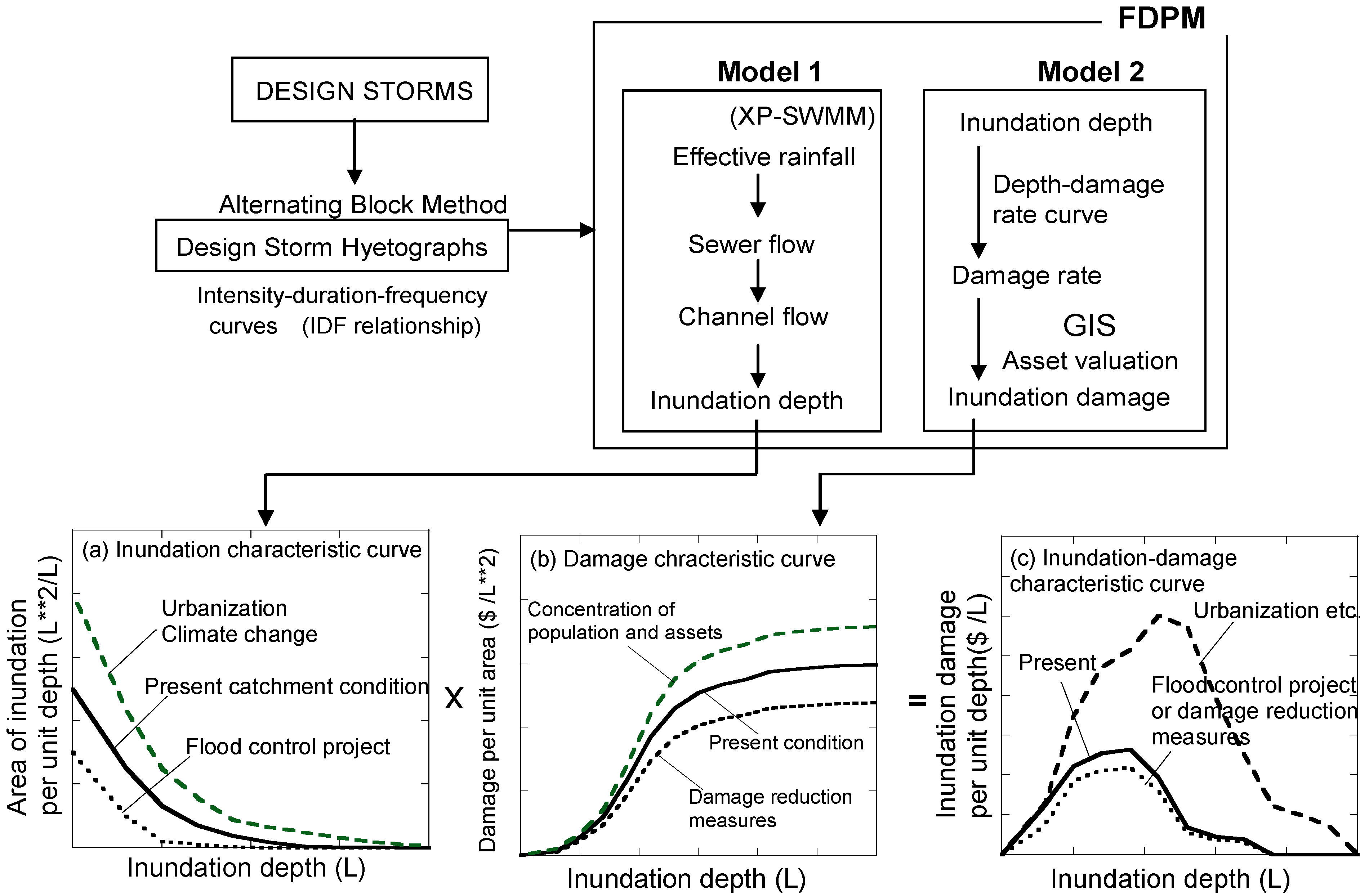
2.1.1. Flood Damage Prediction Model (FDPM)

FDPM, a GIS-based flood damage prediction model, consists of two parts, Model 1 and Model 2. Model 1 calculates two-dimensional inundation depths for input hyetographs. Model 2 estimates monetary inundation damages for any given inundation depths (Figure 1).

For Model 1, XP-SWMM, a stormwater modeling software package for urban drainage [18], is used to calculate inundation depths on a square grid for a given hyetograph. Other flood inundation simulation models can also be used for Model 1.

Model 2 estimates the monetary cost of inundation damage, including direct and indirect damages, as a function of inundation depth. To calculate direct damages, an asset valuation of each item is multiplied by a damage rate determined from the depth-damage rate curve. The asset values of all the items in drainage area are obtained by GIS database. Indirect damage is calculated with the relation between inundation depth and the number of business interruption days for each business. Multiplying the number of days by the employee’s added value per day for each place of business, the indirect damage is obtained for each place.

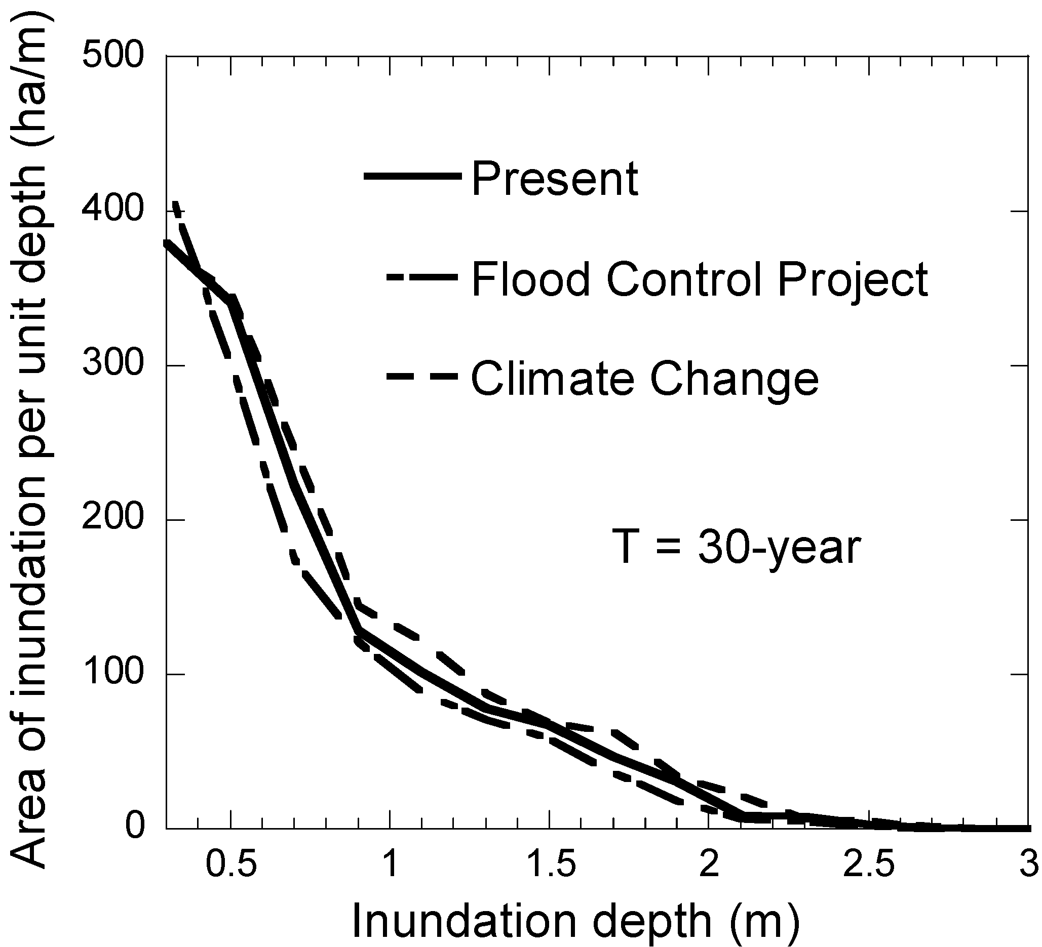
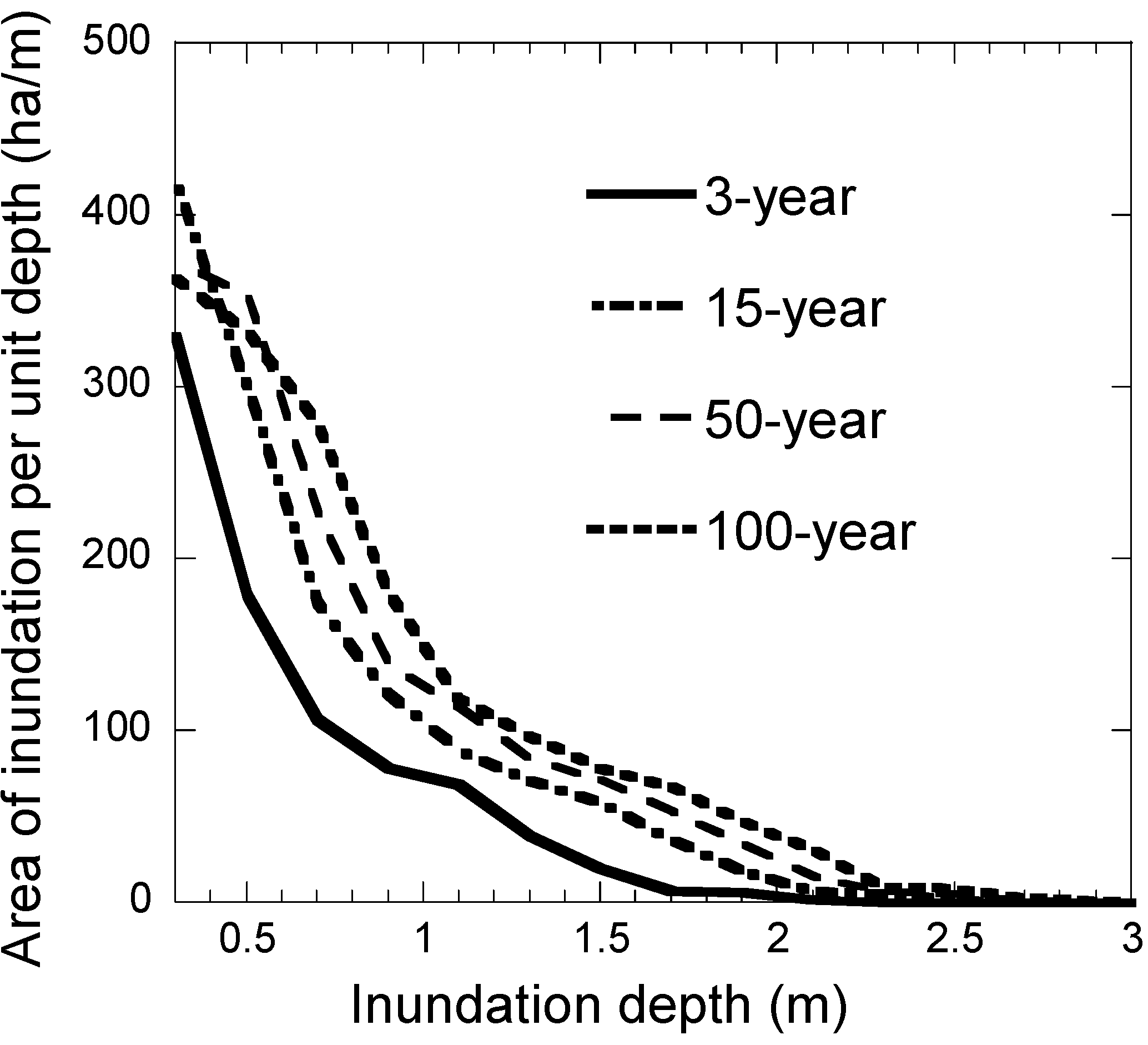
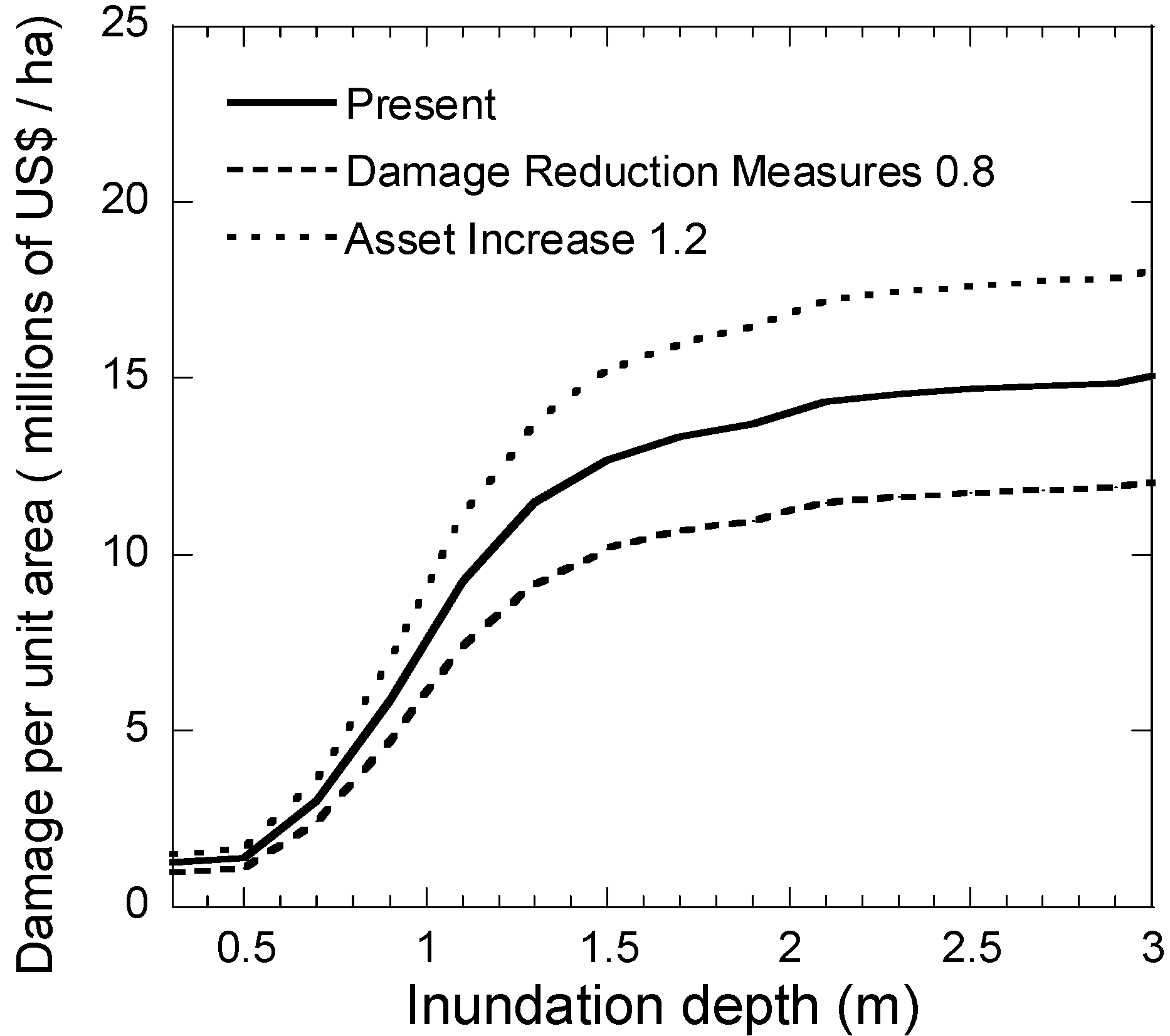
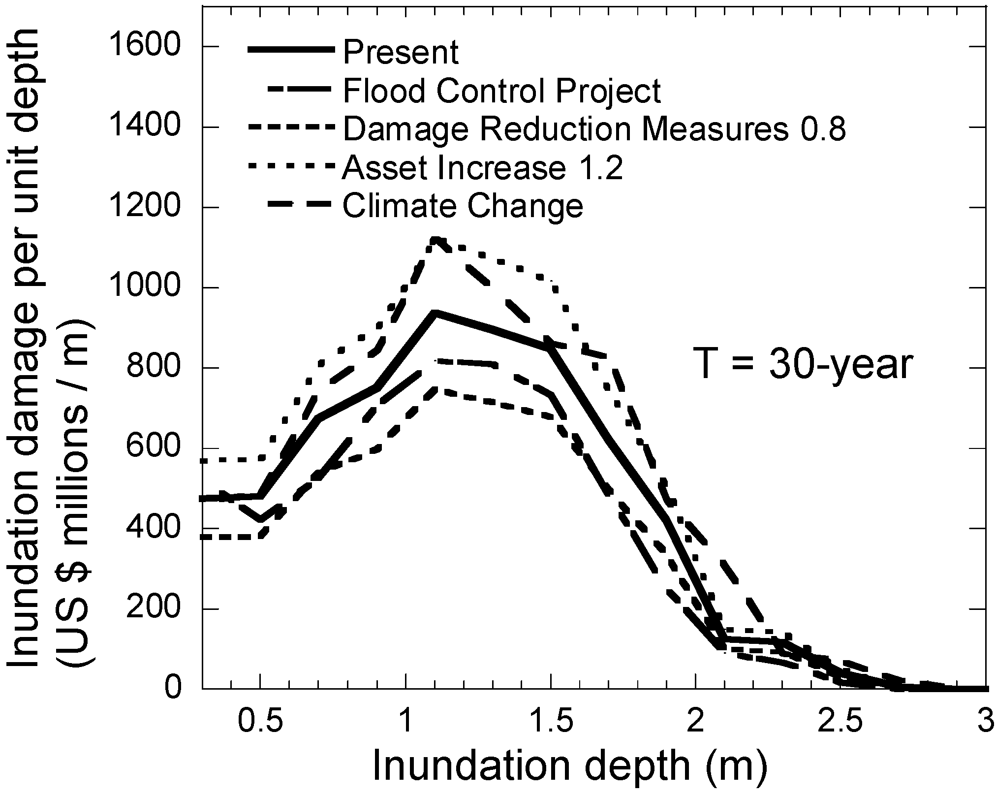
2.1.2. Three Curves for Inundation and Damage Characteristics

The inundation depths for any given storm are calculated in two dimensions using Model 1. The inundation characteristic curve shows the relationship between inundation depth and the flooded area per unit depth for different return period storms. The curves are shown for only one return period in Figure 1a. If we want know the area of inundation depth from d₁ to d₂, we then integrate area of inundation per unit depth between depth d₁ and d₂. In the FDPM calculation, the integral of the curve equals the total area inundated in the catchment.

For the inundation characteristic curve, the solid line shows the inundation for present catchment conditions as in Figure 1a. Urbanization and global warming shift the present inundation upward as shown by the dashed lines. Conversely, flood control projects decrease the inundation as shown by the dotted lines.

The monetary costs of inundation are estimated for any given inundation depth using Model 2 as shown in Figure 1. The damage characteristic curve gives the relationship between the inundation depth and monetary inundation damage per unit area averaged for the catchment (Figure 1b). Catchments have various land uses and the population and assets are not distributed uniformly. This curve can well be used for catchments that are relatively spatially homogeneous.

Monetary inundation damage is calculated by multiplying a value from the inundation characteristic curve by the appropriate value from the damage characteristic curve. This produces a new curve called the inundation-damage characteristic curve, which shows the relationship between inundation depth and monetary damage per unit depth over the whole catchment for one return period storm (Figure 1c). The integral of the curves for different return periods gives the monetary damages for storms having different return periods. The results are used to devise the damage potential curve described below.

The inundation and damage characteristics for a catchment are described by the three curves. These curves reflect the natural and social aspects of the catchment.

2.2. Flood Risk Analysis

The flood risk analysis uses three curves: a storm probability curve, a damage potential curve, and an annual risk density curve (Figure 2). In the flood risk analysis, multiplying the storm probability curve by the inundation damage potential curve produces the annual risk density curve. The risk density curve gives useful information on flood risk characteristics and risk cost.

Figure 2. Three curves used in flood risk analysis: (a) Damage potential curve; (b) Storm probability curve; and (c) Risk density curve.

Figure 2. Three curves used in flood risk analysis: (a) Damage potential curve; (b) Storm probability curve; and (c) Risk density curve.

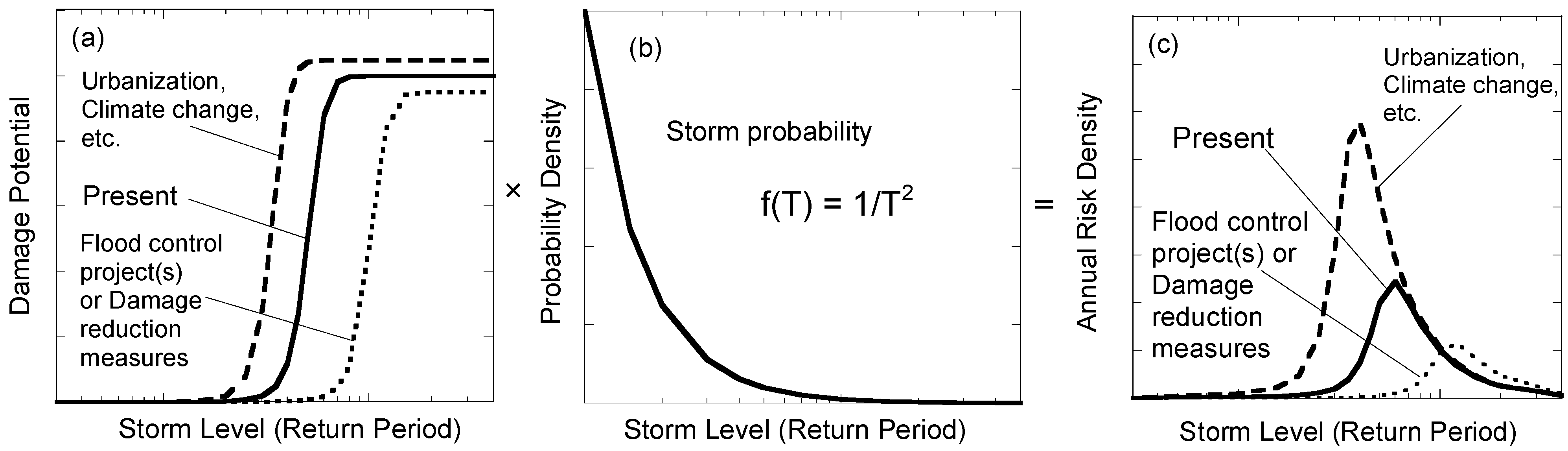
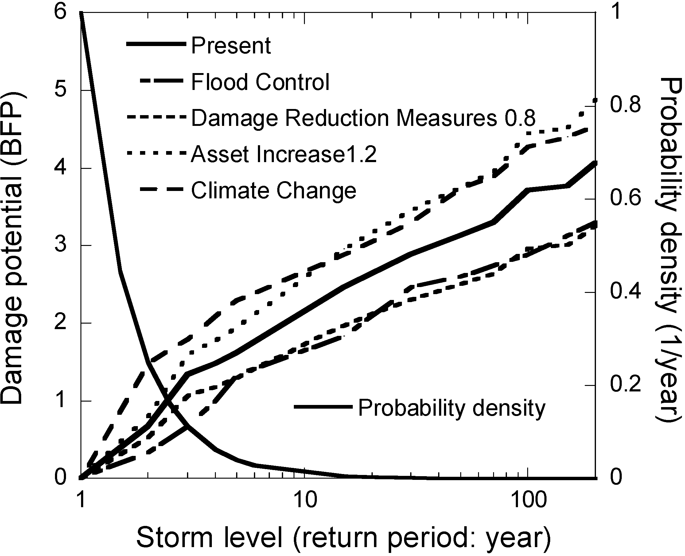
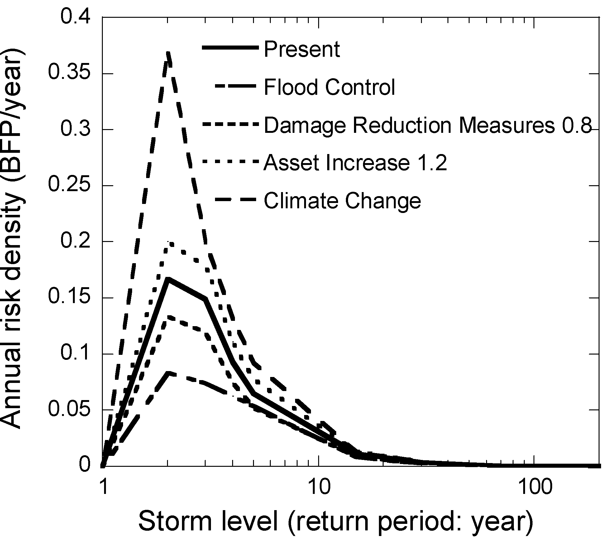
2.2.1. Three Curves for Flood Risk Analysis

The results of integrating the inundation-damage characteristic curves for different return periods are plotted as a damage potential curve, which shows the relationship between the design storm return period and flood damage as in Figure 2a. The damage potential curve can also be calculated directly from the FDPM using a GIS assets database, when land use and asset distribution in the catchment are not homogeneous [16].

The design storms used in the FDPM simulations are specified by their return periods. The return period T and cumulative probability P are related by the equation P = 1 − 1/T. Thus, the probability density is f(T) = 1/T², as given in Figure 2b.

In our study, flood risk is defined as the product of flood inundation damage and the probability of its occurrence. Thus, flood inundation risk is quantified using estimates of monetary damage caused by the design storm and that storm’s probability of occurring. The annual risk density curve, which has a peak in the middle as shown in Figure 2c, is, thus, obtained by multiplying the increasing damage potential curve and the decreasing storm probability curve.

The three curves describe the flood risk characteristics for a catchment.

2.2.2. Flood Risk Interconnections

FDPM simulations for different return period storms provide inundation and damage characteristic curves. Both characteristic curves are linked to the inundation-damage characteristic curve. The integrals of the inundation-damage characteristic curves for different return periods are transformed into the damage potential curve. The product of the damage potential curve and the storm probability curve produces the annual risk density curve.

The three curves obtained by the FDPM simulations shift with changes in catchment conditions. Similarly, the damage potential curve shifts upward due to urban development, global climate change, and increased assets, and downward as flood control projects and flood damage reduction measures are implemented, as shown in Figure 2a. Changes in the damage potential curve are, in turn, linked with the risk density curve as shown in Figure 2c.

The six curves are, as stated above, interconnected and reflect the effects of urbanization, climate change, structural and non-structural flood prevention measures, and other positive or negative factors.

2.3. Flood Risk Assessment

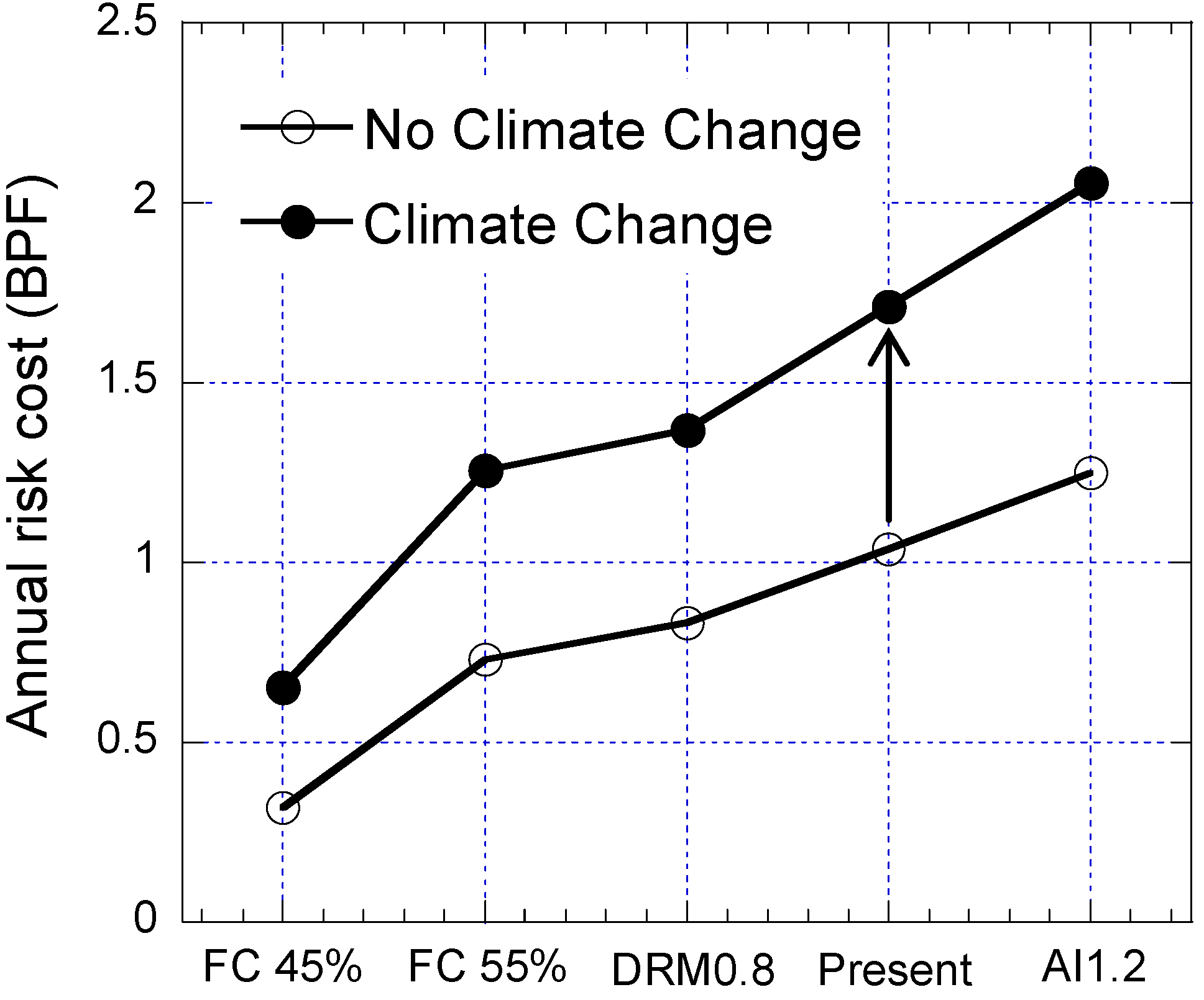
2.3.1. Flood Risk Cost

In this study, risk cost is used to mean the risk as defined in monetary terms for the annually averaged expenditure over time incurred for flood inundation damage. The risk cost depends on the annual risk density curve and is obtained by integrating the risk density curve with respect to return period.

The flood risk cost for present catchment conditions decreases as flood control projects are implemented and increases with global climate change because heavy storms are expected to become more frequent due to global warming.

The risk costs for present catchment conditions and future conditions are RC₀ and RC, respectively. The change in flood risk cost should be the difference between the two, ∆RC = RC − RC₀.

2.3.2. Flood Risk Impact Factor (FRIF)

Urban river basins are exposed to various flood risks such as increased impervious area due to urban development and the effects of global climate change. Increased impervious area does not necessarily represent a flood risk itself, but a factor that may affect the flood risk of a specific urban area. Conversely, flood control projects are effective in reducing the flood risk in urban catchments.

The factors that affect risk cost can be evaluated with a single non-dimensional scale of one simple index, FRIF. This is computed as FRIF = (RC − RC₀)/RC₀. A positive FRIF value indicates increased flood risk, while a negative one indicates reduced flood risk. The magnitude of the impact factor indicates the importance of the risk-increasing or risk-decreasing effects of changing conditions in urban catchment areas.

3. Application of Flood Risk Assessment

This flood risk assessment method was applied to the Kiba drainage area located in Koto Ward in the Tokyo metropolis. The Kiba drainage area has an area of 6 km² characterized by a combined sewer network with a flat topography facing the Tokyo bay. The drainage area has a high population density and numerous assets. The land use and the distribution of population and assets in the drainage area are almost homogeneous. Figure 3 shows the outline of the Kiba Drainage area.

Figure 3. Kiba drainage area and calculated inundation depth for a 15-year return period storm under present catchment condition with GIS data superposed.

Figure 3. Kiba drainage area and calculated inundation depth for a 15-year return period storm under present catchment condition with GIS data superposed.

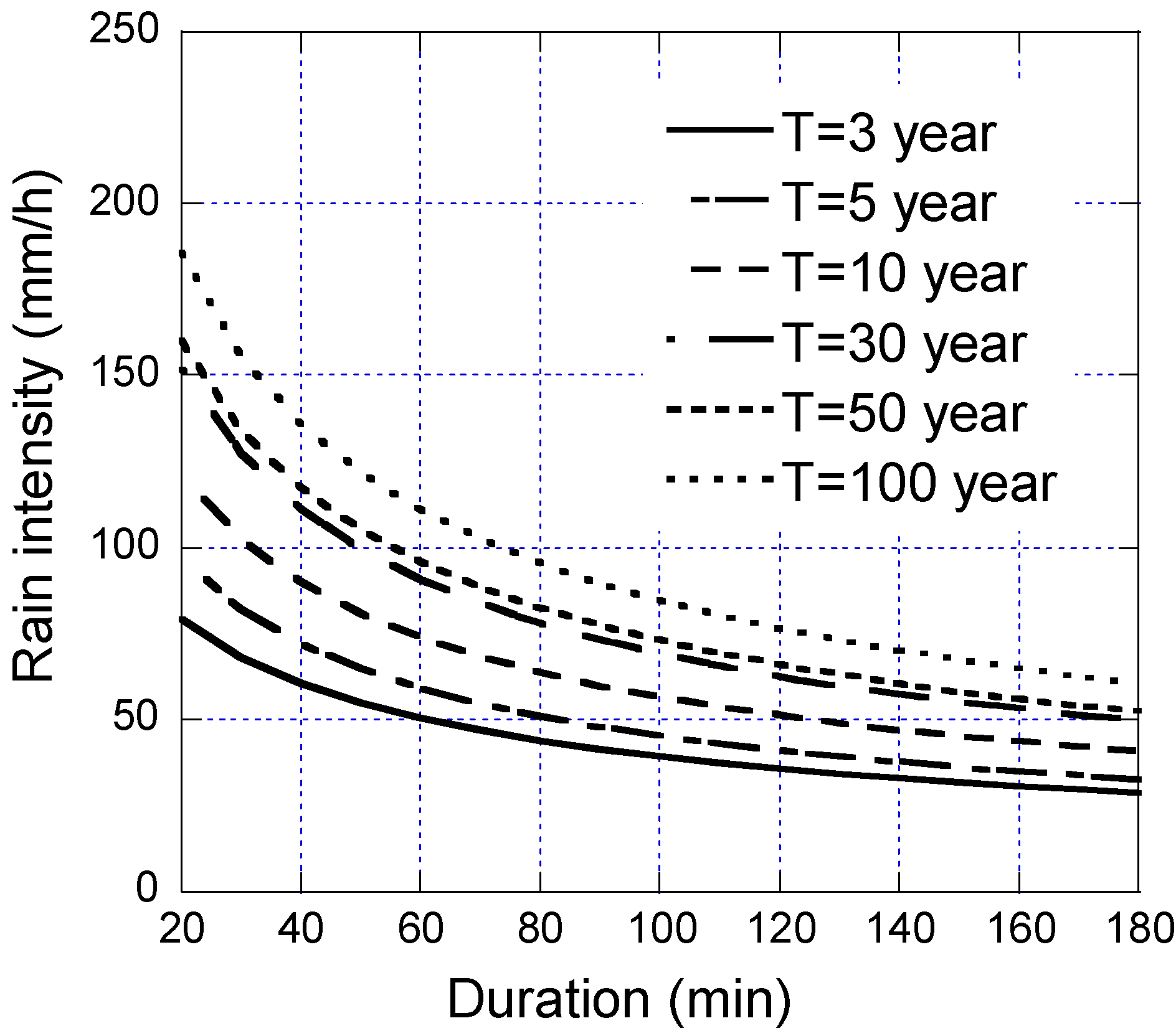
3.1. Design Storms for FDPM Simulation

The FDPM simulation uses a set of design storm hyetographs having various return periods. Each hyetograph input into the FDPM is created form the IDF relationship for its corresponding return period using the alternating block method [19]. These hyetographs have a peak in the middle. The IDF curves for the study were determined by the Gumbel distribution and adopted by the Tokyo Metropolitan Government. Figure 4 shows some examples of IDF curves for some different return periods representing present storm conditions.

Figure 4. Variation of Intensity-Duration-Frequency relationships and return period.

Figure 4. Variation of Intensity-Duration-Frequency relationships and return period.

Design storms for the simulations have return periods of 3, 5, 15, 30, 50, 70, 100, 150, 200, 300, and 500 years. Input hyetographs with a duration of 12 h were created based on IDF curves for storms with these 11 return periods using the alternating block method.

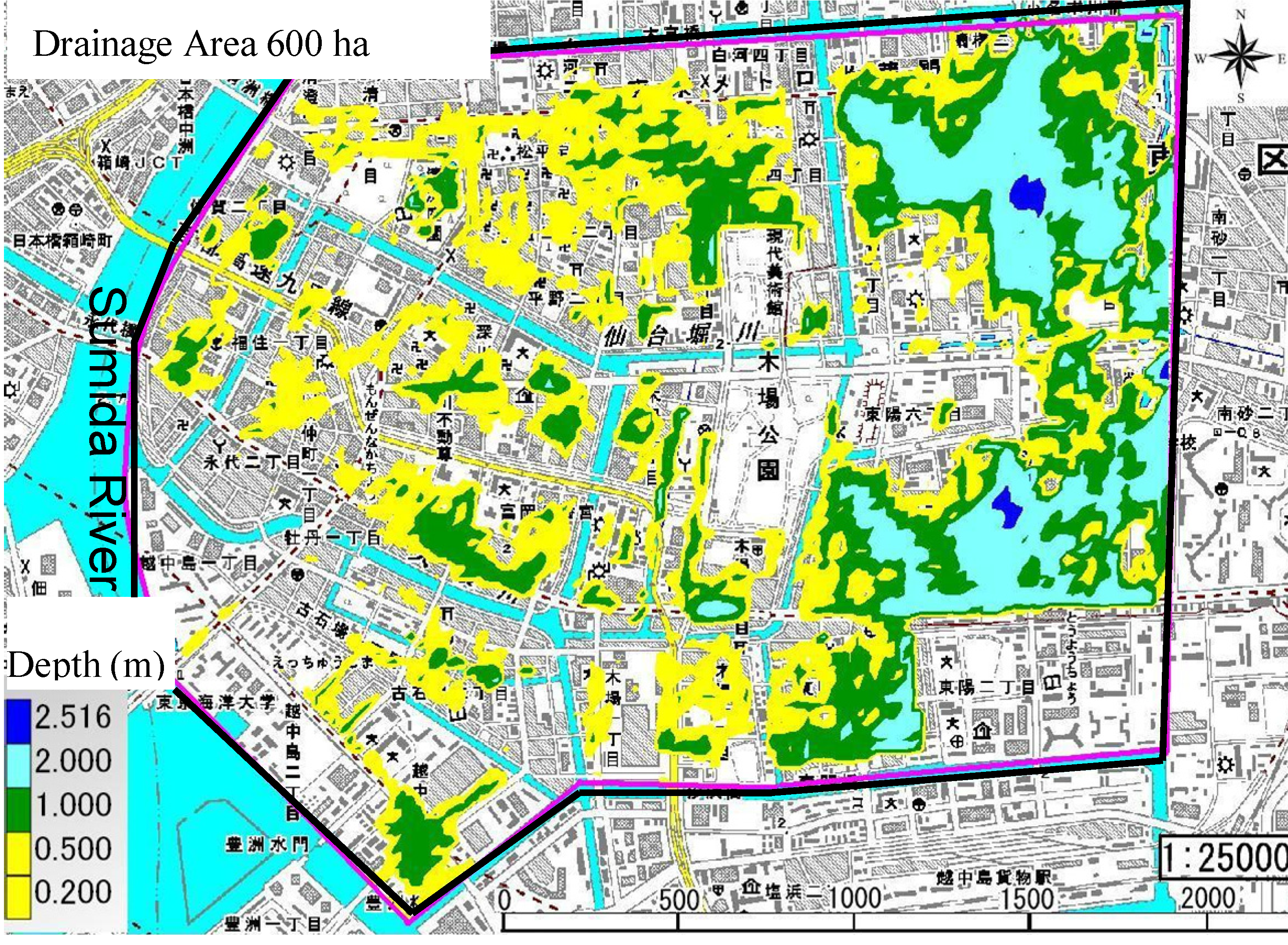
3.2. Flood Inundation Damage Simulation by FDPM

Figure 1 shows the FDPM simulation calculation procedure. Flood inundation depths and damages were calculated using Models 1 and 2 for changes in catchment conditions and global climate changes.

For Model 1, we used XP-SWMM to calculate the inundation depths two-dimensionally on a 10-m square grid for a given hyetograph. The time increment ∆t was set to be 1.0 s for calculation stability. There were 392 nodes and 404 grid cells. The inundation water was assumed to flow on the natural surface according to the Geographical Survey Institute of Japan’s 10 m digital elevation model (DEM). The roughness coefficients were set be 0.03 for pervious area and 0.01 for impervious area. The water’s pathways and detailed land use were taken into account by adjusting the roughness coefficients up to 0.1. The hydraulic model (Model 1) using XP-SWMM was calibrated by comparing the calculated inundation depths with the inundation depths under a historical storm shown in the hazard map of Koto Ward in the Tokyo metropolis [20]. An example of an FDPM inundation simulation is shown in Figure 3 for a 15-year return period storm with current catchment conditions. The FDPM simulation for each return period storm produces a T-return period inundation characteristic curve as shown in Figure 1a. The FDPM, using XP-SWMM, calculates not only inundation depths but also floodwater velocities. Flood risk was evaluated not only from inundation depth but also from floodwater velocity in some studies [21]. In our study, the velocities were not considered for the flood damage estimation because the Kiba drainage area is almost flat with a slope of around 10⁻⁴. If a drainage area has complicated topography with steep slopes in some areas, we have to consider the velocities calculated by Model 1 for the flood risk evaluation.

Monetary damages are calculated by Model 2, using the relationship between inundation depth and damage rate for the eleven different types: four types for building structures and seven types for movables. The calculation methods of Model 2 are explained in Morita [22]. For the catchment-based macro-assessment in this study, we calculate the inundation damages of all the assets under the condition that the inundation depth is uniformly the same for the whole drainage area, summing up all of the inundation damages of the assets. Thus, the whole damage of the drainage area can be calculated for all specified inundation depths. The calculated damages per unit area are plotted with respect to different inundation depths and then one curve is obtained as a damage characteristic curve. The damage characteristic curve shows the spatially averaged characteristics over the drainage area. The averaged inundation damage for a catchment is estimated using a GIS database available from the Tokyo Metropolitan Government.

Model 2 uses a relationship between inundation depth and damage rate to estimate flood damage in monetary basis as stated above. This basic idea for flood damage estimation seems to be internationally accepted as the standard approach to assess urban flood losses [23]. However, not only inundation depth but also floodwater velocity has an effect on flood risk. Smith [21] shows some critical combinations of inundation depth and flow velocity for building failure for three different building types. Kreibich et al. [23] analyzed in detail the influence of flow velocity along with inundation depth on monetary flood loss, primarily of residential buildings. They concluded that water depth is an important parameter for monetary loss estimation as it is commonly used on loss modeling and that general consideration of flow velocity in monetary loss modeling cannot be recommend on the basis of their study. They also indicate that flow velocity have a considerable effect on flood damage in road infrastructure. In our study, we estimated flood risk on the monetary basis for the residential and business buildings. Damage modeling should have different approaches for monetary or non-monetary loss and for different types of direct or indirect flood damages.

3.3. Change in Present Catchment Conditions

The change in urban catchment conditions is likely to bring about more flooding and social impacts to cities and the people living in them. Hammond et al. [24] present a framework for flood impact assessment in urban areas, categorizing flood damage into tangible, intangible, direct and indirect damage, and so on. In the study, the impacts are broadly categorized and dealt with to quantify the flood risk in urban drainage areas.

Inundation damage in the Kiba drainage area could be reduced if steps were taken to improve inland flooding. It is extremely urbanized, with 65% of its area being impervious. Flood control projects such as storm storage reservoirs and infiltration facilities would be equivalent to reducing the impervious area from 65% to lower rates, such as 55% and 45%. The FDPM simulations deal with two cases, in which flood control projects reduce the impervious area to 55% and 45% of the total catchment.

If the assets in the area were concentrated even more, the cost of flood inundation damage would increase. In the simulations, the case where assets increase by 20% is also calculated. The damage characteristic curve shown in Figure 1b would shift upward in that case. Conversely, measures to reduce flood damage, such as removing furnishings and industrial appliances, would reduce the damage to assets in private houses and business buildings. In the simulations, a maximum 20% reduction was assumed considering the situation of the assets and people’s activities in the area during the storm.

3.4. Change in Storm Characteristics Due to Global Climate Change

There is now much meteorological research working on predicting changes in the characteristics of storms due to global warming. Little, however, focuses on the changes in magnitude and frequency of heavy storms in the Tokyo region in terms of IDF relationships. Only two studies have produced such results, both based on general circulation models (GCMs): the National Institute for Land and Infrastructure Management (NILIM) [25] and Oki [26] of the Institute of Industrial Science (IIS) of Tokyo University.

To assess the impact of climate change, risk assessment using FDPM simulations needs not only current design hyetographs but also predicted hyetographs after global warming. This means IDF relationships should be estimated for global climate change. Nguyen et al. [14] presented a spatial and temporal downscaling method based on GCMs in detail and estimated the resulting variation in IDF curves. In the study, the author uses a simple return period shift (RPS) method to estimate flood damage for global climate change [16,17].

The change in flood risk cost due to global warming is determined by the increase in inundated areas as shown by the inundation characteristic curves in the flood risk assessment (Figure 1a). To estimate the area inundated when climate change has occurred, we use the relationship between design storm return periods before and after global warming. Oki [26] estimated the annual maximum daily precipitation, for the 20th and 21st centuries, in the Tokyo metropolis, and presented an important relationship between return periods for the 20th and 21st centuries for the Tokyo metropolitan area. The 21st and 20th centuries are hereinafter referred to as with and without global climate change, respectively. For example, in Figure 5, a 50-year return period storm before global warming corresponds to a 20-year return period storm after global warming. The inundation characteristic curve computed for a 50-year return period can be interpreted as corresponding to a 20-year return period storm after global warming. Similarly, the inundation characteristic curve after climate change can be determined from that for the present conditions by referring to the corresponding return periods. The RPS method, thus, easily creates an inundation characteristic curve representing conditions after global climate change from the present inundation characteristic curve.

The RPS method can also be used to create a damage potential curve for post-global climate change conditions directly from the present damage potential curve for non-homogeneous drainage areas [16].

Figure 5. Return periods for 20th and 21st centuries (Oki [23]).

Figure 5. Return periods for 20th and 21st centuries (Oki [23]).

4. Results and Discussion

The results of the FDPM simulations produced the three inundation and damage characteristic curves shown in Figure 1. The three curves were followed by three risk analysis curves: a damage potential curve, a storm probability curve, and an annual risk density curve. Finally, we computed the flood risk costs and FRIF for changes in catchment conditions and global climate.

4.1. Inundation and Damage Characteristic Curves

The inundation characteristic curve gives the relationship between inundation depth and its area per unit depth. Figure 6 shows the relationship for a 30-year return period storm for three cases: present catchment conditions, flood control projects reducing the impervious area to 55%, and global climate change using the RPS method. Naturally, shallower inundation covers a larger area. The flood control projects decrease the inundation area by producing less impervious area, but conversely, inundation area grows as there are expected to be heavier storms under climate change.

The inundation characteristic curves are calculated for different return period storms. Figure 7 shows the inundation characteristic curves for some return periods under present catchment conditions. The higher return period storms cause deeper inundation and larger inundated areas. For an inundation depth of 0.3 m, the areas for 100-year and 50-year return period storms are smaller than that for a 15-year return period storm. This can be explained by the flat topography of the Kiba drainage area. The 100-year storm causes more area to be inundated to depths over 0.3 m than does the 15-year storm.

Figure 6. Inundation characteristic curves for present catchment condition, a flood control project, and climate change.

Figure 6. Inundation characteristic curves for present catchment condition, a flood control project, and climate change.

Figure 7. Inundation characteristic curves for different return period storms and present catchment conditions.

Figure 7. Inundation characteristic curves for different return period storms and present catchment conditions.

The damage characteristic curve is shown in Figure 8. A larger inundation depth is associated with greater inundation damage. The upper dotted line reflects the asset valuation of the catchment and shows damages increased by 20%. The lower dashed line, conversely, indicates how much the damage would decrease if damage reduction measures during storm periods were undertaken.

Figure 8. Damage characteristic curves for present catchment conditions, damage reduction measures (−20% in assets), and with assets increased by 20%.

Figure 8. Damage characteristic curves for present catchment conditions, damage reduction measures (−20% in assets), and with assets increased by 20%.

Figure 9 shows the inundation-damage characteristic curve that relates inundation damage to inundation depth. The curve is obtained by multiplying the inundation characteristic and damage characteristic curves. We can easily see that most damage occurs at an inundation depth of 1.1 m. The first floor levels of the buildings seem to be at heights of about 0.5 m from the ground. Most of the household articles for private houses and the assets for business buildings are located on the first floor. This means most of the damage is due to inundated household articles for private houses and inundated depreciable and inventory assets for business buildings.

Figure 9. Inundation-damage characteristic curves for present catchment conditions, flood control projects, damage reduction measures, asset increases, and climate change.

Figure 9. Inundation-damage characteristic curves for present catchment conditions, flood control projects, damage reduction measures, asset increases, and climate change.

4.2. Damage Potential Curve and Annual Risk Density Curve

The damage potential curve shows the relationship between storm levels expressed by return period and their cost of monetary inundation damage. The curve is created by integrating the inundation-damage characteristic curve for each return period and then plotting them for different return periods.

The RPS method was applied to the inundation characteristic curve using the relationship shown in Figure 5. For example, the 3-year, 15-year, 50-year, and 100-year return period curves in Figure 7 can be translated into 1.5-year, 6.5-year, 20-year, and 40-year return period curves, respectively. Finally, the return period shifts of the inundation characteristic curves were reflected in the damage potential curves after climate change. The damage potential curves for conditions after climate change were thus obtained from the inundation characteristic curves through the integrations of the inundation-damage characteristic curves, taking climate change into consideration.

Figure 10 shows the damage potential curve and the storm probability curve for the drainage area. The monetary costs of flood damage are expressed in non-dimensional form. BFP in Figure 10 is the unit of the non-dimensional value of the monetary cost of flood damage. We can obtain the damage potential expressed in the unit BFP, dividing the monetary cost by the average budget for flood prevention of the Tokyo Metropolitan Government, approximately 240 million US$.

The annual risk density curves were computed by multiplying the damage potential and storm probability curves shown in Figure 10. The damage potential curves indicate how each flood cause increases or decreases in damage. Figure 11 shows the annual risk density curves for present catchment conditions, flood control projects, damage reduction measures, increased assets, and global climate change. The risk density curves are highest at 2 years. The risk density grows with increased assets and climate change and drops when flood control projects and flood reduction measures are assumed. The curve for climate change has the largest risk among the factors.

Figure 10. Storm probability curve and damage potential curves for present catchment conditions, flood control projects, damage reduction measures, asset increases, and climate change.

Figure 10. Storm probability curve and damage potential curves for present catchment conditions, flood control projects, damage reduction measures, asset increases, and climate change.

Figure 11. Annual risk density curves for present catchment conditions, flood control projects, damage reduction measures, asset increases, and climate change.

Figure 11. Annual risk density curves for present catchment conditions, flood control projects, damage reduction measures, asset increases, and climate change.

4.3. Risk Cost and Risk Cost Change

Flood risk costs were calculated by integrating the annual risk density curves for the five conditions (FC45%, FC55%, DRM0.8, AI1.2, and Present), with and without global climate change. Figure 12 shows the calculated results. FC45% and FC55% mean flood control projects to achieve impervious rates of 55% and 45%, respectively, down from the present 65%. DRM0.8 denotes measures to reduce damage by 20%. AI1.2 indicates assets increased by 20%.

Figure 12. Annual risk costs for present catchment conditions, flood control projects, damage reduction measures, increased assets, and climate change. FC45% and FC55%: flood control projects; DRM0.8: damage reduction measures; and AI1.2: asset increase.

Figure 12. Annual risk costs for present catchment conditions, flood control projects, damage reduction measures, increased assets, and climate change. FC45% and FC55%: flood control projects; DRM0.8: damage reduction measures; and AI1.2: asset increase.

The risk cost grows as assets increase, but decrease when flood control projects are undertaken. The risk cost for current catchment conditions increases by a remarkable 70% due to global warming and the risk costs for the other catchment conditions (FC45%, FC55%, DRM0.8, AI1.2) have similar trends.

4.4. Flood Risk Impact Factor (FRIF)

FRIF is easily computed using the calculated risk costs given in Figure 12. Figure 13 shows the risk cost and associated FRIF values for the various catchment conditions. Closed and open circles, respectively, denote conditions with and without global climate change. When written in italics, FC45%, FC55%, DRM0.8, and AL1.2 denote conditions under climate change. The FRIF values indicate the impacts of urbanization, flood control projects, damage reduction measures, and climate change as a simple index.

Figure 13. Flood risk impact factors for present catchment conditions, flood control projects, damage reduction measures, asset increases, and climate change. FC45% and FC55%: flood control projects; DRM0.8: damage reduction measures; and AI1.2: increased assets.

Figure 13. Flood risk impact factors for present catchment conditions, flood control projects, damage reduction measures, asset increases, and climate change. FC45% and FC55%: flood control projects; DRM0.8: damage reduction measures; and AI1.2: increased assets.

Current conditions have an annual risk cost of about 1 BFP and an FRIF of 0.0. The effect of increasing assets by 20% (AI1.2) has the same value, 0.25, as that of building flood control projects that lower the impervious area to 55% combined with global warming (FC55%). Flood control projects to lower the impervious area to 45% (FC45%) more than balance the risk cost increase due to global warming because the FRIF is negative. The FRIF goes up to 1.0 when assets are increased by 20% and climate change is assumed (AI1.2). All in all, climate change, among the four causes, should be the most effective to increase the flood risk. Thus, the FRIF gives useful information on how various causes either increase or decrease flood risk, and on synergistic effects of various factors with regard to urban river management.

The FRIFs calculated in the risk assessment can be used in decision-making processes. The well-informed decision making, however, depends on the quality of the assessment. It is, thus, important to have an understanding of uncertainty related to flood risk assessment [27]. In the early period of the flood damage reduction studies by the US Army Corps, the uncertainty was already taken into account in the flood risk analysis technique [6]. Apel et al. [28], and de Moel et al. [29] emphasized the importance to quantify the uncertainty in flood risk assessment and thus tried to evaluate the main sources of uncertainty in the assessment processes. They indicate that uncertainty in the damage calculation has a relatively large effect on the damage estimates as compared to other categories of parameters: hydraulic condition, flood frequency, inundation characteristics, exposure characteristics, and future scenarios. In this study, the damage calculations are clearly connected with the calculations of flood risk cost. Therefore it would be better that the calculated results as shown in Figure 8, Figure 9, Figure 10, Figure 11 and Figure 12 were expressed not in deterministic form but in probabilistic form based on the uncertainty analysis. Actually the uncertainty analysis using FDPM (Figure 1) would require a huge amount of computation time for the flood risk assessment in the study. The effect of uncertainty on the values of FRIF in Figure 13 would, however, be to some extent mitigated because the FRIFs are expressed in non-dimensional form to comparatively evaluate the main causes to contribute to flood risk. For future scenarios, the return period shift (RPS) method was taken to consider the effect of global warming on flood risk in the study. The effect of uncertainty in future scenarios should be the most important because the change in storm characteristics owing to climate change has large uncertainty.

5. Concluding Remarks

The objective of the study was to present a risk assessment method for evaluating and comparing the main factors contributing to flood risk in urban drainage areas. The most important results are as follows:

(1)

We present a risk assessment method that employs a GIS-based FDPM and the XP-SWMM routine, and can evaluate factors that increase and decrease the risk of urban flooding to serve as a basis for urban drainage management;

(2)

The risk assessment method was employed to estimate the reduction in flood risk provided by flood control projects and damage reduction measures and the increased risk due to asset increases and global climate change in the Kiba drainage area of the Tokyo metropolis;

(3)

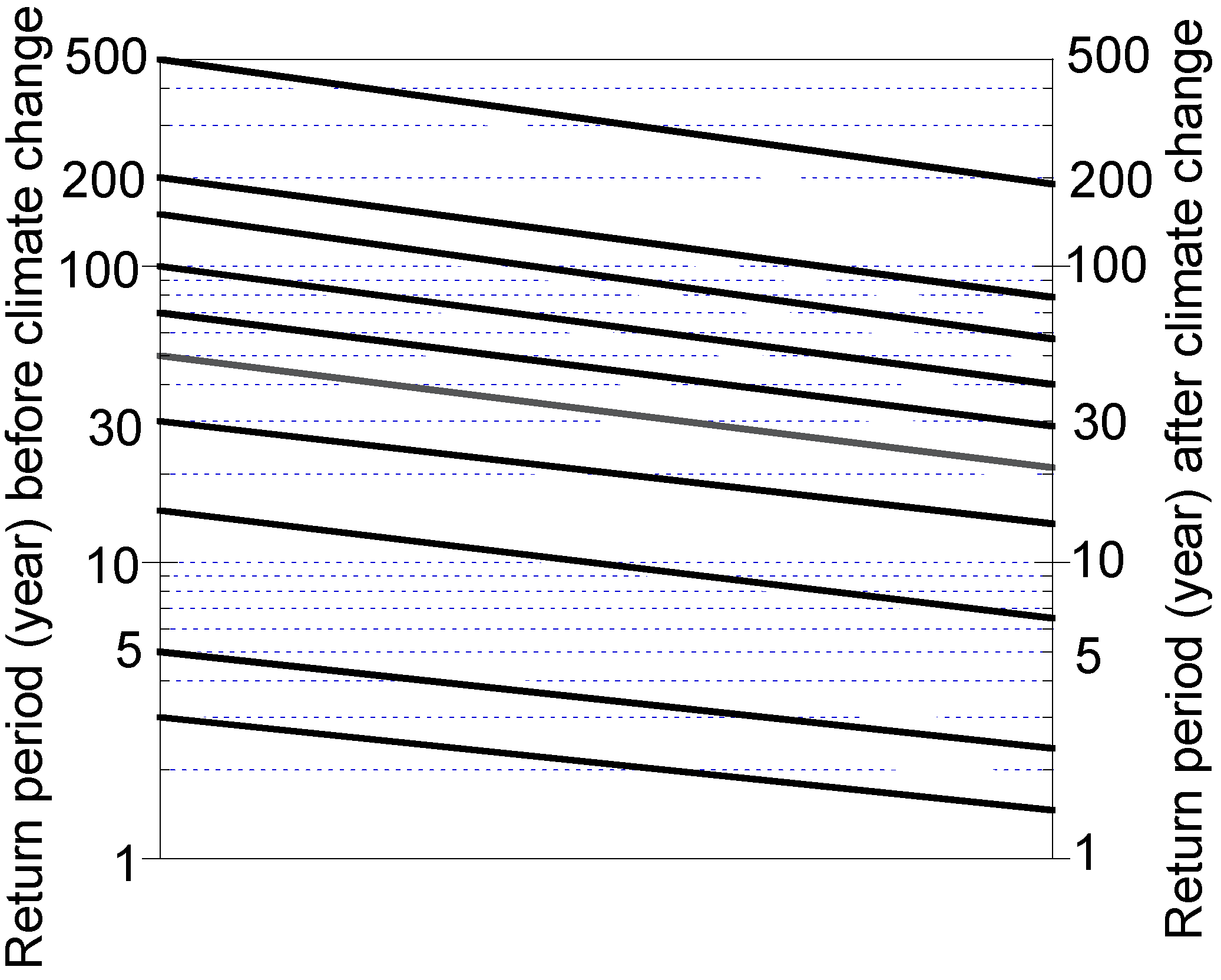
The RPS method was applied as a simple way to estimate the flood damage potential of global warming, based on present conditions without climate change;

(4)

FRIF was introduced as an index to evaluate the effectiveness of various sources of increased or reduced flood inundation risk to our society. Risk impact factors calculated from FDPMs may play an important role in urban flood prevention planning and decision-making processes.

References

1. Intergovernmental Panel on Climate Change (IPCC). Climate Change 2007: Fourth Assessment Report Climate Change 2007 Synthesis Report, Topic3. Available online: http://www.ipcc.ch/pdf/assessment-report/ar4/syr/ar4_syr.pdf (accessed on 14 September 2009).
2. Patrick, W.; Jonas, O.; Karsten, A.-N.; Simon, B.; Assela, P.; Ida Bulow, G.; Henrik, M.; Van-Thanh-Van, N. Impacts of Climate Change on Rainfall Extremes and Urban Drainage Systems; IWA Publishing: London, UK, 2007. [Google Scholar]
3. Wilson, R. Analyzing the daily risks in life. Technol. Rev. 1979, February, 41–45. [Google Scholar]
4. National Research Council. Improving Risk Communications; National Academy Press: Washington, DC, USA, 1999.
5. Crichton, D. Role of insurance in reducing flood risk. Geneva Pap. 2008, 33, 117–132. [Google Scholar]
6. National Research Council. Risk Analysis and Uncertainty in Flood Damage Reduction Studies; National Academy Press: Washington, DC, USA, 2000; p. 179.
7. Baan, P. Risk Perceptance and Preparedness and Flood Insurance. In Urban Flood Management, Chapter 6, Urban Flood Management; Szollosi-Nagy, A., Zevenbergen, C., Eds.; Taylor & Francis Group plc.: London, UK, 2005; pp. 67–82. [Google Scholar]
8. Samuels, P.G. Where Next in Flood Risk Management? A Personal View on Research Needs and Directions. In Proceedings of 2nd European Conference on Flood Risk Management, Flood Risk 2012. Rotterdam, The Netherlands, 19–23 November 2013.
9. Klijn, F.; Samuels, P.; Van Os, A. Towards flood risk management in the EU: State of affairs with examples from various European countries. Int. J. River Basin Manag. 2008, 6, 307–321. [Google Scholar] [CrossRef]
10. Davis, D.W. Risk analysis in flood damage reduction studies—The corps experience. In Proceedings of the Congress of Environmental and Water Resources Institute, Philadelphia, PA, USA, 23–26 June 2003.
11. Morita, M. Flood risk analysis for determining optimal flood protection levels in urban river management. J. Flood Risk Manag. 2008, 1, 142–149. [Google Scholar] [CrossRef]
12. Plate, E.J. Flood risk and flood management. J. Hydrol. 2002, 267, 2–11. [Google Scholar] [CrossRef]
13. Department for Environment Food and Rural Affairs (DEFRA). Climate Adaptation: Risk, Uncertainty and Decision-Making. In UKCIP Technical Report; Willows, R.I., Connell, R.K., Eds.; UKCIP (UK Climate Impact Programme): Oxford, UK, 2003. [Google Scholar]
14. Nguyen, V.-T.-V.; Nguyen, T.-D.; Cung, A. A statistical approach to downscaling of sub-daily extreme rainfall processes for climate-related impacts studies in urban areas. Water Sci. Technol. Water Supply 2007, 7, 183–192. [Google Scholar] [CrossRef]
15. Morita, M. Quantification of increased flood risk due to global climate change for urban river management planning. Water Sci. Technol. 2011, 63, 2967–2974. [Google Scholar] [CrossRef]
16. Morita, M. Risk assessment method for flood control planning considering global climate change in urban river management. IAHS Publ. 2013, 357, 107–116. [Google Scholar]
17. Morita, M. Flood Risk Impact Factor for Flood Risk Assessment in Urban River Management. In Proceedings of the 2nd European Conference on Flood Risk Management, Floodrisk 2012. Rotterdam, The Netherlands, 19–23 November 2013.
18. Phillip, B.C.; Yu, S.; de Silva, N. 1D and 2D Modeling of Urban Drainage Systems Using XP-SWMM and TUFLOW2. In Proceedings of the 10th International Conference on Urban Drainage, Copenhagen, Denmark, 22–25 August 2005.
19. Chow, V.T.; Maidment, D.R.; Mays, L.W. Applied Hydrology; McGraw-Hill Science: New York, NY, USA, 1988. [Google Scholar]
20. Koto city. The Hazard Map. Available online: http://www.city.koto.lg.jp/seikatsu/douro/7509/13389/file/map.pdf (assessed on 15 October 2013).
21. Smith, D.I. Flood damage estimation—A review of urban stage-damage curves and loss functions. Water SA 1994, 20, 231–238. [Google Scholar]
22. Morita, M. Risk analysis and decision—Making for optimal flood protection level in urban river management. In Proceedings of the European Conference on Flood Risk Management, Floodrisk 2008. Oxford, UK, 30 September–2 October 2008.
23. Kreibich, H.; Piroth, K.; Seifert, I.; Maiwald, H.; Kunert, U.; Schwarz, J.; Merz, B.; Thieken, A.H. Is flow velocity a significant parameter in flood damage modelling? Nat. Hazards Earth Syst. Sci. 2009, 9, 1697–1692. [Google Scholar]
24. Hammond, M.J.; Chen, A.; Butler, D.; Djordjević, S.; Manojlović, N. A framework for flood impact assessment in urban areas. IAHS Publ. 2013, 357, 41–47. [Google Scholar]
25. National Institute for Land and Infrastructure Management. Projection of Future Storm Rainfall Intensity Affected by Global Climate Change—Analysis of GCM20 Model Simulation Results; Technical Note of NILIM, No.462; National Institute for Land and Infrastructure: Tsukuba, Japan, 2008; pp. 107–116.
26. Oki, T. Localized torrential rainfall and flood disaster in urbanized area. J. Hydrol. Syst. 2008, 61, 5–9, in Japanese. [Google Scholar]
27. Pappenberger, F.; Beven, K.J. Ignorance is bliss: Or seven reasons not to use uncertainty analysis. Water Resour. Res. 2006, 42. [Google Scholar] [CrossRef]
28. Apel, H.; Merz, B.; Thieken, A.H. Quantification of uncertainties in flood risk assessments. Int. J. River Basin Manag. 2008, 6, 149–262. [Google Scholar] [CrossRef]
29. De Moel, H.; Aerts, J.C.J.H. Effect of uncertainty in land use, damage models and inundation depth on flood damage estimates. Nat. Hazards 2011, 58, 407–425. [Google Scholar] [CrossRef]