A Web-Based Model to Estimate the Impact of Best Management Practices

1
Department of Agricultural and Biological Engineering, Purdue University, 225 South University Street, West Lafayette, IN 47907-2093, USA
2
Earth, Atmospheric, and Planetary Sciences, Purdue University, 550 Stadium Mall Dr., West Lafayette, IN 47907, USA
*
Author to whom correspondence should be addressed.
Water 2014, 6(3), 455-471; https://doi.org/10.3390/w6030455
Submission received: 24 January 2014
/
Revised: 25 February 2014
/
Accepted: 7 March 2014
/
Published: 13 March 2014
Abstract
:The Spreadsheet Tool for the Estimation of Pollutant Load (STEPL) can be used for Total Maximum Daily Load (TMDL) processes, since the model is capable of simulating the impacts of various best management practices (BMPs) and low impact development (LID) practices. The model computes average annual direct runoff using the Soil Conservation Service Curve Number (SCS-CN) method with average rainfall per event, which is not a typical use of the SCS-CN method. Five SCS-CN-based approaches to compute average annual direct runoff were investigated to explore estimated differences in average annual direct runoff computations using daily precipitation data collected from the National Climate Data Center and generated by the CLIGEN model for twelve stations in Indiana. Compared to the average annual direct runoff computed for the typical use of the SCS-CN method, the approaches to estimate average annual direct runoff within EPA STEPL showed large differences. A web-based model (STEPL WEB) was developed with a corrected approach to estimate average annual direct runoff. Moreover, the model was integrated with the Web-based Load Duration Curve Tool, which identifies the least cost BMPs for each land use and optimizes BMP selection to identify the most cost-effective BMP implementations. The integrated tools provide an easy to use approach for performing TMDL analysis and identifying cost-effective approaches for controlling nonpoint source pollution.
1. Introduction
Section 303(d) of the Clean Water Act requires states and other defined authorities to develop lists of impaired rivers and streams that have seriously contaminated water. They need to establish priority rankings for waters on the lists and to develop Total Maximum Daily Loads (TMDLs). Various models have been used not only to develop TMDLs, but also to perform analyses to identify strategies to attain pollutant load limits with plans typically identifying best management practices (BMPs) to reduce loads [1,2,3,4,5,6].
One such model is the Spreadsheet Tool for the Estimation of Pollutant Load (STEPL), which computes average annual direct runoff, sediment load, nutrient loads and five-day biological oxygen demand (BOD5) [7]. The model is capable of estimating average annual non-point source (NPS) pollutant loads, and in addition, the model allows estimation of impacts of various BMP implementations and low impact development (LID) practices, so that pollutant load reduction for BMPs or LIDs can be computed [7,8,9,10]. EPA STEPL requires land use and the hydrologic soil group (HSG) to define the curve number (CN), as it computes direct runoff in a watershed based on the Soil Conservation Service Curve Number (SCS-CN) method [11]. Land use categories in the model are urban, cropland, pastureland, forest and user defined.
However, the model uses processes that are not scientifically based on calculating average annual direct runoff, and the average annual direct runoff is used to estimate average annual NPS pollutant loads. Thus, the runoff, pollutant loads and BMP impacts predicted by EPA STEPL are questionable. The first unscientific process is the use of precipitation to compute direct runoff based on average rainfall per event calculated by Rainfall, Rain Days, Precipitation Correction Factor, and Number of Rain Days Correction Factor for each county [7]. However, the SCS-CN method is typically used to simulate event- or daily-based direct runoff using specific daily rainfall in hydrologic models [12,13,14,15,16]. EPA STEPL calculates direct runoff for a rainfall value (i.e., ‘average rainfall per event’) with the SCS-CN method, and then, the model multiplies the direct runoff from that rainfall by ‘Rain Days’ and ‘Number of Rain Days Correction Factor’ to reproduce average annual direct runoff. This approach may not be appropriate to accurately reproduce long-term average annual direct runoff. It is questionable to estimate average annual direct runoff obtained using average rainfall values (i.e., average rainfall per event) with CNs, since the relationships between CNs and rainfall are not linear [17,18].
The second unscientific process employed in STEPL is the selection of the default initial abstraction coefficient (λ) for the SCS-CN method. The SCS-CN method equations are as follows [18].
![Water 06 00455 i001]()
![Water 06 00455 i002]() where, Q is direct runoff (mm), P is precipitation (mm), Ia is initial abstraction (mm) and λ is the initial abstraction coefficient.
where, Q is direct runoff (mm), P is precipitation (mm), Ia is initial abstraction (mm) and λ is the initial abstraction coefficient.

Q = 0 for P ≤ Ia

Ia = λ × S
The initial abstraction coefficient typically varies from 0.0 to 0.2 [19,20]. The CN tables published and currently used typically assume that the initial abstraction coefficient is 0.2. If a different initial abstraction coefficient is used, the CN values need to be adjusted [14,21]. The EPA STEPL default for the initial abstraction coefficient is 0.0, while the denominator of Equation (1) in EPA STEPL is fixed as “P + 0.8 S”, thus making the implementation of the equation incorrect. Further, STEPL does not adjust CNs when initial abstraction is updated by users. Although the EPA STEPL model allows changing the initial abstraction coefficient, if the user leaves it as the default, this will likely result in overestimation of runoff and, therefore, overestimation of average annual pollutant loads, because the direct runoff calculated with a value of 0.0 S for initial abstraction with a fixed denominator is greater than the direct runoff calculated with a value of 0.2 S for initial abstraction. Most significantly, it is incorrect to use a modified initial abstraction value with the CNs provided in standard references, as these are for an initial abstraction of 0.2 S [18]. However, EPA STEPL estimates average annual direct runoff using an initial abstraction of 0.0 S and the CNs provided in standard references. If an adjustment of initial abstraction is made, CN and S both need to be adjusted based on the change to initial abstraction. This is because the initial abstraction coefficient was empirically determined to be 0.2 [18], and Equations (1)–(4) need to be modified when other initial abstraction coefficient values are used [14,21].
EPA STEPL is a spreadsheet model for not only average annual pollutant load estimation, but also simulation of BMP impacts. A model capable of simulating BMPs was required for the Web-based Load Duration Curve Tool (Web-based LDC Tool; [22]), since the Web-based LDC Tool is not capable of simulating BMPs to meet the standard pollutant loads, although the Web-based LDC Tool identifies pollutant loads exceeding standards and computes the required pollutant reduction to meet the standard loads. Moreover, the Web-based LDC Tool identifies BMPs with the least cost for each land use, but the BMPs and area to which these practices should be applied need to be optimized for cost-effective BMP implementation. Therefore, the objectives of the study were: (1) to examine and correct the average annual direct runoff approach in EPA STEPL; and (2) to develop a web-based model capable of simulating pollutant load reductions for BMPs.
2. Methodology
The study had two purposes: one was to examine the average annual direct runoff approach in EPA STEPL to identify the impacts of its assumptions on runoff computations and corresponding pollutant loads; and the other was to develop a web-based model that used a load duration curve tool and the corrected STEPL for identifying appropriate BMPs and simulating their effects on pollutant load reduction. Five approaches to estimate average annual direct runoff with the SCS-CN method were explored. Daily precipitation data from twelve National Climate Data Center (NCDC, [23]) stations were collected for conducting the analyses. The first approach was to obtain average annual direct runoff by aggregating daily direct runoff computed by the SCS-CN method and NCDC daily precipitation data. The second and third approaches represented current EPA STEPL approaches using values of 0.0 and 0.2 for initial abstraction coefficients. In the fourth approach, daily precipitation data were generated by the CLIGEN model [24], and average annual direct runoff was computed from daily direct runoff obtained using daily precipitation data. The fifth approach was using the EPA STEPL model.
For the second objective of the study, a web-based model was developed based on a corrected EPA STEPL model. The web-based model provides web interfaces and employs the CLIGEN model to generate daily precipitation data. Modules to calibrate model parameters and to optimize BMPs were developed and integrated in the web-based model.
2.1. Average Annual Direct Runoff Computations
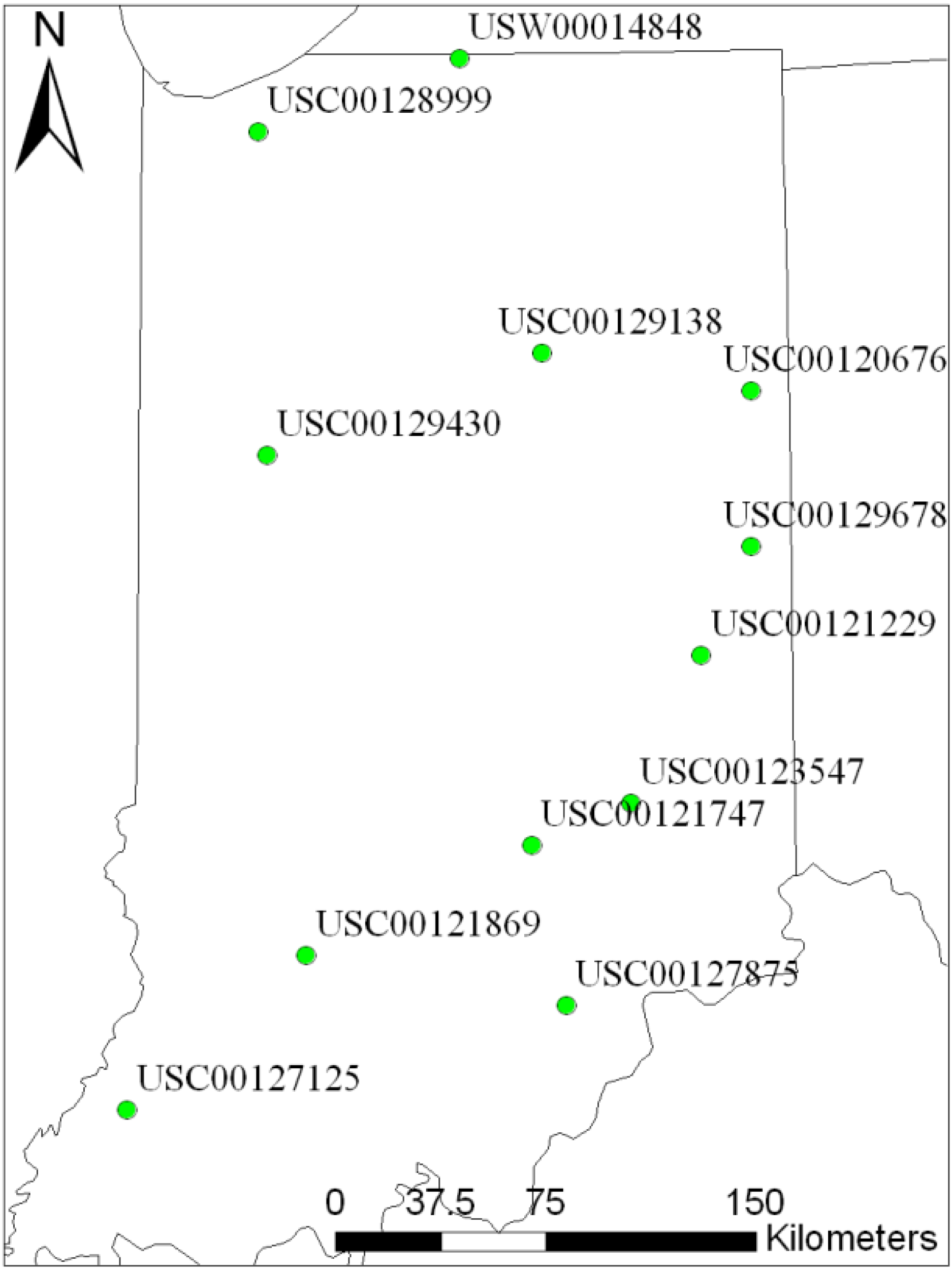
Daily precipitation data were collected from the NCDC to explore the approaches to compute average annual direct runoff using measured daily precipitation data. Daily precipitation data were generated with the CLIGEN model using the inputs collected from the United States Department of Agriculture (Table 1, Figure 1). Twelve NCDC stations providing long-term daily data were selected within Indiana, and twelve CLIGEN stations were selected, which are geographically identical to the NCDC stations.
Five approaches to compute average annual direct runoff were established. The approaches were to investigate the average annual direct runoff differences between the methods: (1) using daily precipitation data with Equations (1)–(4); (2) using average rainfall per event with Equations (5)–(7) (described below) and an initial abstraction coefficient of 0.0 (i.e., the original EPA STEPL method); (3) using average rainfall per event with Equations (5)–(7) and an initial abstraction coefficient of 0.2 (i.e., corrected EPA STEPL method); (4) using daily precipitation data generated by the CLIGEN model with Equations (1)–(4); and (5) using the EPA STEPL model.
![Water 06 00455 i003]()
![Water 06 00455 i004]()


Average Annual Direct Runoff Depth = ARD × Rain Days × Rain Days Correction Factor
The first approach used Equations (1)–(4) to compute daily direct runoff depth with daily precipitation data from NCDC with an initial abstraction coefficient of 0.2. In other words, the approach was to represent the general use of the SCS-CN method to compute average annual direct runoff depth.
The second and third approaches were to represent the average annual direct runoff depth computations in EPA STEPL. The EPA STEPL database related to precipitation data was not used for the second and third approaches, thus preventing possible average annual direct runoff differences due to precipitation data differences, because the purpose of this step was the comparison of approaches. If the EPA STEPL database had been used, the approaches would have been incomparable, because different precipitation data would have led to different average annual direct runoff estimates. Therefore, the required inputs (i.e., average annual rainfall, rain days, and correction factors for Equation (5)) in the second and third approaches were computed based on the daily precipitation data collected from NCDC for each location. Rainfall correction factors are the percentage of precipitation greater than 5 mm; the factors were computed by dividing the sum of daily precipitation values greater than 5 mm by the sum of daily precipitation values. Rain day correction factors are the percentage of rain days that have precipitation greater than 5 millimeters [7]. Average rainfall per event (ARE) was computed using Equation (5). An initial abstraction coefficient of 0.0 was used for Equation (6) in the second approach to compute average annual direct runoff depth, while the initial abstraction coefficient in the third approach was 0.2.

| Station Number | Station Name | Period |
|---|---|---|
| USC00120676 | Berne WWTP | 1949–1999 |
| USC00121747 | Columbus | 1921–2010 |
| USC00121869 | Crane NSA | 1943–1959 |
| USW00014848 | South Bend Michiana Regional Airport | 1948–2012 |
| USC00128999 | Valparaiso Waterworks | 1985–2000 |
| USC00129138 | Wabash | 1989–2004 |
| USC00129430 | West Lafayette 6 NW | 1989–2012 |
| USC00129678 | Winchester AAP 3 | 1989–2012 |
| USC00121229 | Cambridge City 3 N | 1975–1992 |
| USC00123547 | Greensburg | 1933–1941 |
| USC00127125 | Princeton 1 W | 1898–1952 |
| USC00127875 | Scottsburg | 1897–2000 |
Figure 1.
Location Map of NCDC and CLIGEN stations within Indiana.

The fourth approach to compute average annual direct runoff used Equations (1)–(4) with daily precipitation data generated by CLIGEN. The fourth approach was identical to the first approach, except that daily precipitation data generated by CLIGEN were used in the fourth approach. The EPA STEPL model, the fifth approach, was used to compute average annual direct runoff with the model database providing average annual rainfall, rainfall correction factor, rain days and the rain day correction factor for the counties in which NCDC stations are located.
2.2. Web Interfaces and CLIGEN Use
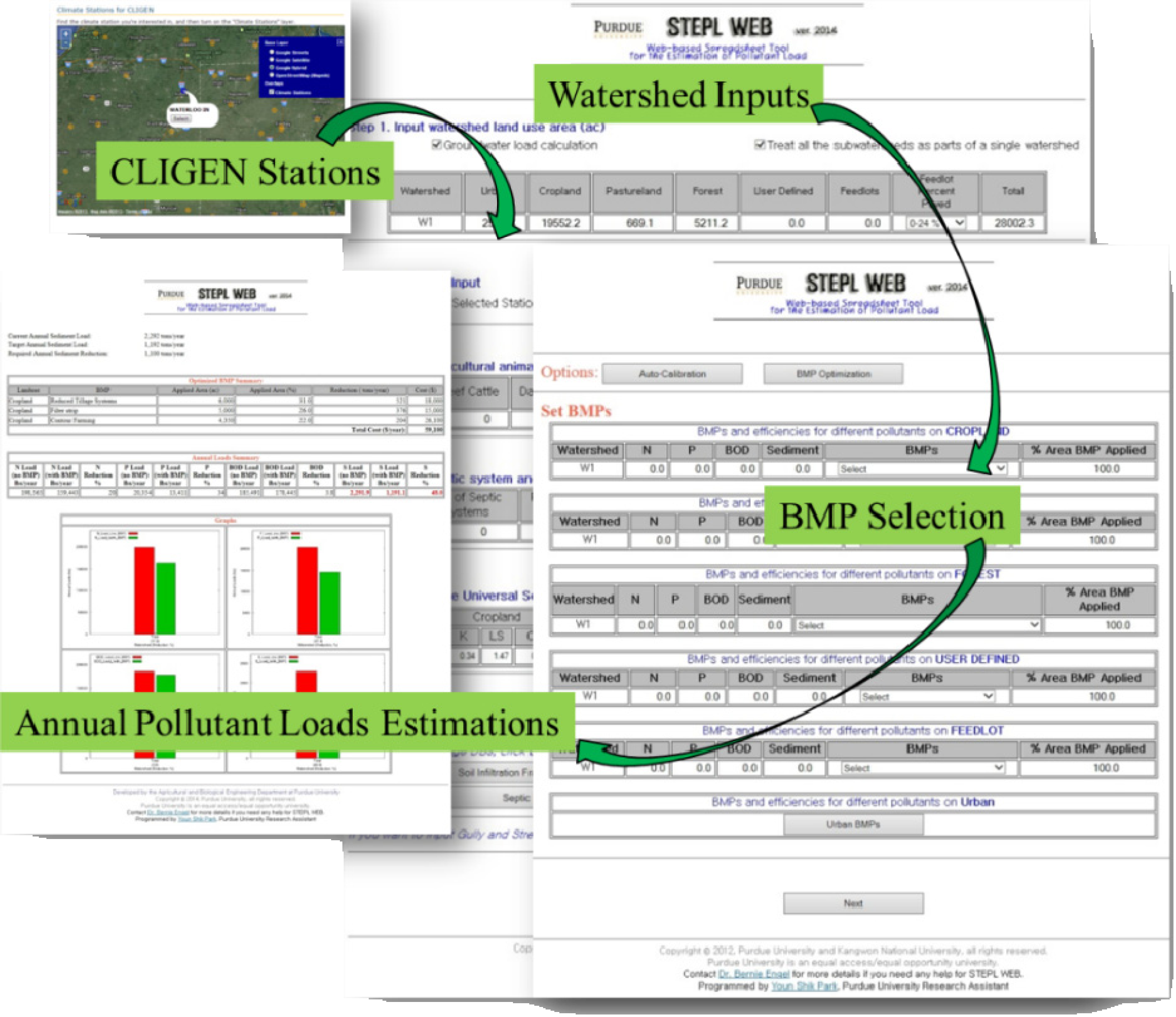
The EPA STEPL model includes a database to provide the input parameters describing precipitation and soil erosion estimation, and the model also has a user-friendly interface within Microsoft Excel. A web-based model (STEPL WEB) was developed following a similar program flow to EPA STEPL, which is to define subwatershed characteristics and then to identify watershed inputs and BMPs in turn. However, HTML interfaces instead of Visual Basic and MS Excel interfaces were created, with the core engine programmed in the FORTRAN programming language to perform the calculations computed in MS Excel in EPA STEPL (Figure 2). A number of Python CGIs and Java Script-based HTML were programmed to handle inputs from databases. Similar to EPA STEPL, the watershed inputs (Figure 2) include land use areas, agricultural animal numbers, septic tank failure rate, irrigation amount, etc. The BMPs/LIDs available in EPA STEPL [7] (Table 2) are also provided in STEPL WEB.
Figure 2.
Web-based Spreadsheet Tool for the Estimation of Pollutant Load (STEPL) (STEPL WEB) interfaces and annual pollutant loads estimation. BMP, best management practice.
Figure 2.
Web-based Spreadsheet Tool for the Estimation of Pollutant Load (STEPL) (STEPL WEB) interfaces and annual pollutant loads estimation. BMP, best management practice.

EPA STEPL computes average annual direct runoff using Equations (5)–(7), but it was replaced with two approaches in the web-based tool. One uses 0.2 S for the initial abstraction, because CNs commonly available and used are based on a value of 0.2 S for the initial abstraction. The other approach employs CLIGEN to generate long-term, daily precipitation data. In addition, the CLIGEN model showed reasonable means and standard deviations of daily precipitation amounts when 100 years of precipitation data were generated [25]. The model performed well with 20 years of precipitation data generation for annual amounts, monthly amounts and the number of events [26]. In addition, the model was employed to generate climate data for a web-based model [27]. Therefore, the web-based model employs CLIGEN for daily precipitation data generation and provides 2368 locations with CLIGEN inputs collected from the United States Department of Agriculture. The daily precipitation data generated by CLIGEN are used to compute daily direct runoff, and daily direct runoff are aggregated to estimate average annual direct runoff in STEPL WEB.
Table 2.
Best management practices and low impact development practices in EPA STEPL and STEPL WEB. LID, low impact development.
| Land use | Best Manage Practices and Low Impact Development Practices |
|---|---|
| Cropland | Contour Farming, Diversion, Filter Strip, Reduced Tillage Systems, |
| Stream Bank Stabilization and Fencing, Terrace | |
| Forest | Road Dry Seeding, Road Grass and Legume Seeding, Road Hydro Mulch, |
| Road Straw Mulch, Road Tree Planting, Site Preparation/Hydro Mulch/Seed/Fertilizer, | |
| Site Preparation/Hydro Mulch/Seed/Fertilizer/Transplants, | |
| Site Preparation/Steep Slope Seeder/Transplant, | |
| Site Preparation/Straw/Crimp Seed/Fertilizer/Transplant, | |
| Site Preparation/Straw/Crimp/Net, Site Preparation/Straw/Net/Seed/Fertilizer/Transplant, | |
| Site Preparation/Straw/Polymer/Seed/Fertilizer/Transplant | |
| Feedlots | Diversion, Filter Strip, Runoff Management System, Solids Separation Basin, |
| Solids Separation Basin w/Infiltration Bed, Terrace, Waste Management System, | |
| Waste Storage Facility | |
| Urban | Alum Treatment, Bioretention Facility, Concrete Grid Pavement, Dry Detention, |
| Extended Wet Detention, Filter Strip-Agricultural, Grass Swales, Infiltration Basin, | |
| Infiltration Devises, Infiltration Trench, LID/Cistern, LID/Cistern + Rain Barrel, | |
| LID/Rain Barrel, LID/Bioretention, LID/Dry Well, LID/Filter/Buffer Strip, | |
| LID/Infiltration Swale, LID/Infiltration Trench, LID/Vegetated Swale, LID/Wet Swale, | |
| Oil/Grit Separator, Porous Pavement, Sand Filter/Infiltration Basin, Sand Filters, | |
| Settling Basin, Vegetated Filter Strips, Weekly Street Sweeping, Wet Pond, | |
| Wetland Detention, WQ Inlet w/Sand Filter, WQ Inlets |
2.3. Auto-Calibration Modules
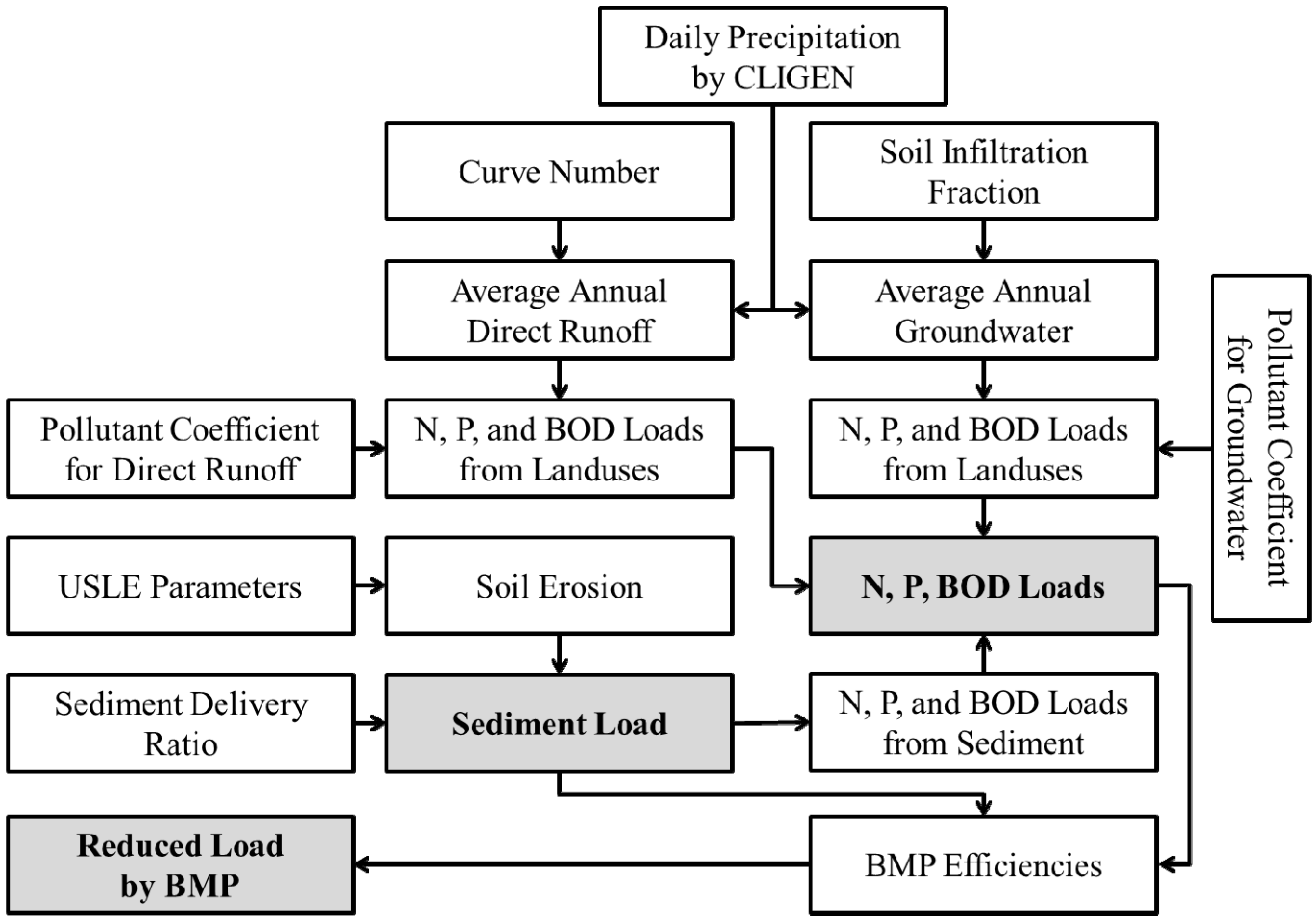
STEPL WEB computes average annual direct runoff using the SCS-CN method, the average annual contribution to shallow groundwater by soil infiltration fractions for precipitation and the average annual pollutant loads by pollutant coefficients multiplied by average annual direct runoff and groundwater (Figure 3). Sediment load is computed based on the Universal Soil Loss Equation (USLE) and sediment delivery ratio (SDR), Equation (10) and (11) [28]. STEPL WEB has two sources of nutrient loads (N, P and BOD). The first source is the nutrient loads from land uses, which are computed by pollutant coefficients and average annual direct runoff and shallow groundwater contribution. The second source is nutrient loads in sediment, which are computed by soil nutrient concentrations and sediment load [7]. Therefore, CNs and soil infiltration fractions should be calibrated for average annual direct runoff and average annual shallow groundwater, so that nutrient loads are correctly computed. Since sediment load is computed by USLE and SDR, the SDR (Equations (10) and (11)) can be calibrated for sediment load. Pollutant coefficients also need to be calibrated for nutrient loads.
Figure 3.
Average annual direct runoff, groundwater and pollutant load computation in STEPL WEB. USLE, Universal Soil Loss Equation; BOD, biological oxygen demand.
Figure 3.
Average annual direct runoff, groundwater and pollutant load computation in STEPL WEB. USLE, Universal Soil Loss Equation; BOD, biological oxygen demand.

Since CNs are defined by land use and HSG, the relationships between CNs need to be maintained. For instance, CNs for urban are typically greater than forest, and CNs for HSG A are smaller than HSG D for a given land use. One approach to calibrate CNs is to multiply default CNs by an identical fraction (or percentage, Frcn in Equation (8)); in other words, CNs are increased or decreased by an identical percentage. Average annual shallow groundwater is computed based on the soil infiltration fractions for precipitation, which are defined by land use and HSG. Therefore, the soil infiltration fractions for precipitation can be calibrated by the approach used for calibrating CNs. The pollutant coefficients are defined by land use, and the calibration approach can be applied (Frnt,1 for N, Frnt,2 for P, and Frnt,3 for BOD in Equation (9)). USLE factors are defined by land uses in STEPL WEB, with factors based on those from the EPA STEPL database. Since sediment loads are computed by multiplying soil erosion (USLE factors) and SDR, sediment loads can be calibrated by SDR calibration rather than by individual USLE factors [29]; the fraction in Equations (10) and (11) is calibrated for average annual sediment load. The fraction is multiplied by SDR, which also implies that USLE factors for soil erosion are increased or decreased by an identical fraction.
Two modules were developed to calibrate the fractions/coefficients in Equations (8)–(11). One module uses a genetic-algorithm (GA), and the other uses the bisection method. The algorithm is based on the principles of natural evolution and survival of the fittest and sets up a population of individuals for a given problem, consisting of a stochastic strategy, which imitates the evolution of natural organisms [30,31]. Solving sophisticated problems effectively, the algorithm has been used for various areas, such as business, engineering and science [32], and is deemed as a powerful method to solve highly complex problems.
The alternative module to calibrate the fractions in Equations (8)–(11) uses the bisection method. The bisection method is a simple and straightforward numerical method, is applicable to continuous functions and has been applied to solve simple problems [33,34,35]. The method sets intervals and selects the midpoint, which shows the least error during iteration, narrowing the intervals. Initial intervals (e.g., 50% to 150% for CNs) need to be set, and iterative computations are required until the error (e.g., the difference between the observed average annual direct runoff and estimated average annual direct runoff) is zero or less than a specified tolerance. The module in STEPL WEB performs the iterations until the intervals are in the thousandth digits for the fractions in Equations (8)–(11):
where Frcn is calibration parameter or fraction for CN, Frnt,i is the calibration parameter for pollutant coefficients, Frsdr is the calibration parameter for SDR and A is the watershed area in square kilometers.
Calibrated CN = Frcn × Default CN
Calibrated Pollutant Coefficient = Frnt,i × Default Pollutant Coefficient
Sediment Delivery Ratio = Frsdr × 0.42 × A−0.135 − 0.127, if A ≥ 0.81
Frsdr × 0.42 × A−0.125, if A < 0.81
2.4. Optimization of Best Management Practices
Since estimated annual cost of BMP implementation in a watershed is computed by BMP cost per unit area and applied area of BMP (AREABMP), both BMP cost and AREABMP need to be considered when identifying the most cost-effective BMP implementation. In other words, the BMP with the least cost per unit mass reduction (i.e., dollars per ton of reduction) needs to be identified and applied, and then, AREABMP needs to be minimized, as long as the estimated reduction meets the required reduction. In addition, use of a BMP on 100% of the land use area may not be possible. For instance, it may not be possible to apply a BMP to 90% of cropland, if the BMP is already applied on 30% of cropland. In this circumstance, the BMP could only be applied to a maximum of 70% of cropland area.
STEPL WEB estimates the BMP implementation cost based on establishment, maintenance and opportunity costs using a cost function Equation (12) [36]. The model computes the costs per unit of pollutant mass reduction for BMPs and establishes a priority list of BMPs to apply based on the cost per unit mass of pollutant reduction.
![Water 06 00455 i005]() where ct is the BMP implementation cost, c0 is the establishment cost, rm is the ratio of the annual maintenance cost to the establishment cost, s is the interest rate and td is the BMP design life.
where ct is the BMP implementation cost, c0 is the establishment cost, rm is the ratio of the annual maintenance cost to the establishment cost, s is the interest rate and td is the BMP design life.

After establishment of the BMP list, STEPL WEB optimizes AREABMP, increasing the AREABMP of the first BMP and estimating average annual pollutant reductions for that BMP. Iterative simulations are required with AREABMP increasing up to the allowable maximum area (e.g., 100% or 70% for the circumstance stated above) until the estimated pollutant reduction is greater than the required reduction. If estimated average annual pollutant reduction for the first BMP does not meet the required reduction, the second most cost-effective BMP needs to be simulated with AREABMP increased iteratively for the second BMP. In brief, the BMP optimization process is an iterative simulation, adding BMPs in turn and increasing AREABMP for each BMP.
3. Results and Discussion
3.1. Average Annual Direct Runoff Computations
To explore the differences in runoff computation approaches, a CN of 85 was selected, which represents cropland with the C hydrologic soil group in the EPA STEPL model. Average annual direct runoff (depth, millimeters) values were computed with the five approaches (Table 3, Figure 4). The average annual direct runoff for the first approach (i.e., general use of the SCS-CN method with daily precipitation data, GU) ranged from 117.4 mm (USC00120676) to 191.4 mm (USC00127125). However, the average annual direct runoff estimated by the second approach (i.e., original EPA STEPL approach, OS) ranged from 242.5 mm (USW00014848) to 339.9 mm (USC00127125). Although identical precipitation data were used for the approaches, the difference between the OS and GU approaches was a minimum of 77.6% (overestimated, USC00127125) and a maximum of 111.8% (overestimated, USC00120676).
| Station | Precipitation (mm) | Average Annual Direct Runoff Depth (mm) | TC8 | |||||
|---|---|---|---|---|---|---|---|---|
| PN1 | PC2 | GU3 | CL4 | CS5 | OS6 | ST7 | ||
| USC00120676 | 963.8 | 940.7 | 117.4 | 107.4 | 41.6 | 248.6 | 216.0 | 78 |
| USC00121747 | 1077.0 | 1027.1 | 164.9 | 147.9 | 68.0 | 309.4 | 327.8 | 76 |
| USC00121869 | 1128.1 | 1146.3 | 187.7 | 189.3 | 76.1 | 334.4 | 331.8 | 76 |
| USW00014848 | 970.7 | 950.5 | 121.1 | 114.5 | 40.2 | 242.5 | 190.7 | 78 |
| USC00128999 | 1008.6 | 958.9 | 152.6 | 121.4 | 56.0 | 274.4 | 218.4 | 76 |
| USC00129138 | 1025.7 | 925.5 | 143.8 | 120.8 | 54.5 | 280.4 | 215.2 | 77 |
| USC00129430 | 996.0 | 935.1 | 145.3 | 125.1 | 55.6 | 274.8 | 215.2 | 77 |
| USC00129678 | 931.3 | 951.8 | 124.8 | 122.6 | 45.8 | 250.8 | 216.2 | 77 |
| USC00121229 | 1044.5 | 1027.8 | 141.1 | 130.3 | 55.6 | 284.4 | 249.1 | 77 |
| USC00123547 | 994.8 | 1047.9 | 129.6 | 144.1 | 48.4 | 263.9 | 327.8 | 77 |
| USC00127125 | 1080.4 | 1069.2 | 191.4 | 176.4 | 85.6 | 339.9 | 357.0 | 75 |
| USC00127875 | 1097.9 | 1078.6 | 173.0 | 161.6 | 69.6 | 320.8 | 335.7 | 76 |
Notes: 1 PN, average annual precipitation from NCDC; 2 PC, average annual precipitation from CLIGEN; 3 GU, average annual direct runoff by daily direct runoff computation; 4 CL, average annual direct runoff with daily precipitation data generated by CLIGEN; 5 CS, EPA STEPL with corrected initial abstraction of 0.2 S; 6 OS, Original EPA STEPL; 7 ST, average annual direct runoff by the EPA STEPL model; 8 TC, curve number threshold to generate direct runoff by CS.
The third approach (i.e., corrected EPA STEPL with an initial abstraction coefficient of 0.2, CS) resulted in underestimation compared to the GU for all stations. Moreover, the approach showed no direct runoff when the average rainfall per event for the stations was smaller than 0.2S calculated by CN (Equation (3)), because the average direct runoff depth (Equation (6)) became 0.0 mm, based on Equation (2). Thus, CN needs to be greater than a critical value (TC (curve number threshold to generate direct runoff by CS) in Table 3) to generate average annual direct runoff greater than 0.0 mm. In other words, there will be no average annual direct runoff in the area with CN values smaller than TC in Table 3.
Figure 4.
Comparison of average annual direct runoff by different approaches.

Daily precipitation data generated by CLIGEN were used to compute daily direct runoff in the fourth approach (CL). The difference between the CL and GU approaches was a minimum of 0.9% (overestimated, USC00121869) and a maximum of 20.5% (underestimated, USC00128999). In addition, the average annual direct runoff from the CL approach demonstrated smaller differences than the average annual direct runoff by the OS and CS approaches.
The EPA STEPL model was used in the fifth approach (ST, average annual direct runoff by the EPA STEPL model), and the estimated average annual direct runoff ranged from 190.7 mm (USW00014848) to 357.0 mm (USC00127125). The difference between the GU and ST approaches was a minimum of 43.1% (overestimated, USC00128999) and a maximum of 152.9% (overestimated, USC00123547). Similar to the OS approach, the ST results showed large differences relative to the GU results.
The results indicate that average annual direct runoff needs to be the aggregate of daily direct runoff based on daily precipitation data. In other words, the approach to compute average annual direct runoff using the SCS-CN method with average rainfall per event (i.e., the OS and CS approaches) would lead to average annual direct runoff that is much larger than values estimated when the CN runoff method is applied as it was intended. Comparing the OS approach to the CS approach, the OS approach showed large differences at all stations, because the denominators in Equation (6) for the OS approach were smaller than those for the CS approach, since the initial abstraction coefficients were 0.0 for OS and 0.2 for CS. Even though the approach using average rainfall per event was corrected (CS), the approach resulted in underestimation compared to the GU approach. In addition, the CS approach estimated average annual direct runoff greater than 0 mm, only when CN was greater than a critical value (TC), and therefore, there will not be average annual direct runoff in areas with small CNs (e.g., forest). The ST approach resulted in not only overestimation of runoff, but also a large difference compared to runoff from the GU approach. Thus, it was concluded that the approach using the average rainfall per event currently used in the EPA STEPL model is not applicable for computing average annual direct runoff.
The SCS-CN method was developed based on the relationship between rainfall and direct runoff [11,18]. SCS-CN is an empirical model composed of two parameters, which are CN and initial abstraction. The initial abstraction was empirically determined to be 0.2 S [18,37]. The CN tables published and currently used typically assume that the initial abstraction coefficient is 0.2. The equations in the SCS-CN method need to be modified when other initial abstractions are used [14,21]. In addition, the SCS-CN method using an initial abstraction coefficient of 0.2 is typically used to simulate daily-based direct runoff using daily rainfall in hydrologic models [12,13,14,15,16].
Since the SCS-CN method is an empirical model, its assumptions must be maintained if it is to provide accurate runoff estimates. Therefore, the initial abstraction needs to be 0.2 S for the CN values commonly used; otherwise, CNs need to be adjusted for other initial abstraction values. The method must also be used for event- or daily-based direct runoff with event- or daily-based rainfall. In other words, average annual direct runoff needs to be computed by aggregating daily direct runoff obtained using daily rainfall. If the assumptions are not maintained in the use of the SCS-CN method, large differences in the results compared to those for the general use of the SCS-CN method may result. For instance, the OS approach used a different initial abstraction (i.e., 0.0S) and did not adjust CNs, and thus, the approach resulted in overestimation compared to the GU approach. When the initial abstraction coefficient was corrected (CS), average annual direct runoff resulted in underestimation compared to the GU approach, because the CS approach used a single rainfall value (average rainfall per event) for average annual direct runoff estimation.
3.2. Application of STEPL WEB
To demonstrate the BMP simulation ability of STEPL WEB, a watershed named the Tippecanoe River at North Webster in northeastern Indiana (Figure 5) was selected. The spatial input datasets to delineate the watershed and to prepare STEPL WEB inputs were the 30-meter resolution digital elevation model (DEM) from the United States Geological Survey (USGS) National Elevation Dataset, the National Land Cover Dataset, 2006 (NLCD 2006), from the USGS, and the Soil Survey Geographic Database (SSURGO) from the United States Department of Agriculture (USDA). The watershed area is 129.1 km2, with 61.3% of the watershed land use being cropland (Figure 5, Table 4).
The Web-based LDC Tool was used to collect flow data from the USGS station number 03330241 (Tippecanoe River at North Webster, IN, USA). Total phosphorus data were collected from the Indiana Department of Environmental Management (IDEM) at the same location. The period selected to develop a load duration curve was from 25 March 1998 to 17 November 2010, based on the water quality data period. The standard concentration for total phosphorus was set to 0.08 mg/L [38]. Average annual direct runoff, average annual baseflow and average annual sediment load were computed with the Web-based LDC Tool. Nutrient loads in STEPL WEB are computed based on loads from runoff, as well as sediment, and therefore, the average annual sediment load is required to calibrate model parameters for average annual nutrient loads. LOADEST [39] was used for average annual sediment load calculation. The model parameters in STEPL WEB were calibrated (Table 5 and Table 6) using the auto-calibration module using the bisection method. The Web-based LDC Tool identified the required phosphorus pollutant reduction percentage to be 11% to meet the standard load. STEPL WEB then established cost-effective BMP lists based on least cost per unit of pollutant reduction. The most cost-effective BMP was filter strip for cropland; reduced tillage systems and contour farming were the second and third most cost-effective BMPs. The fourth and fifth most cost-effective BMPs were vegetated filter strips and bioretention facility for urban.
Figure 5.
Land uses of the Tippecanoe River at North Webster watershed. USGS, United States Geological Survey.
Figure 5.
Land uses of the Tippecanoe River at North Webster watershed. USGS, United States Geological Survey.

| Land use | Area (km2) | Percentage (%) |
|---|---|---|
| Urban | 10.4 | 8.1 |
| Cropland | 79.2 | 61.3 |
| Pasture | 2.7 | 2.1 |
| Forest | 21.1 | 16.3 |
| Water | 15.7 | 12.2 |
| Total | 129.1 | 100.0 |
Two scenarios for BMP application in the watershed were simulated. One was the application of filter strip on up to 79 km2 (100% of the cropland area). The other was the application of filter strip on up to 10 km2 in the cropland area and reduced tillage systems on up to 10 km2 of cropland; contour farming was considered not applicable, and vegetative filter strips were possible on up to 5 km2 in urban area. In the first scenario, filter strip for cropland needed to be applied to 17 km2 of cropland to reach the pollutant reduction goal, with an estimated annual cost of $12,870. In the second scenario, filter strip needed to be applied to 10 km2 of cropland; reduced tillage systems needed to be applied to 10 km2 of cropland, and vegetative filter strips needed to be applied to 4 km2 of urban as the optimal solution. The estimated annual cost was $17,400, which resulted from $7,650 for filter strip, which provided 147.5 kg/year phosphorus reduction in cropland, $7,710 for reduced tillage systems with 95.6 kg/year phosphorus reduction in cropland and $2,040 for vegetative filter strips with 1.0 kg/year phosphorus reduction in urban. Both scenarios met the required reduction; however, the estimated annual cost of the second scenario was more expensive than the first scenario, but the first scenario may not be feasible if ‘filter strip’ application is not possible to implement on 17 km2 or more of cropland area.
| Model Parameters | HSG | A | B | C | D |
|---|---|---|---|---|---|
| Curve Number | Urban | 83/90 | 89/97 | 92/98 | 93/98 |
| Cropland | 67/73 | 78/85 | 85/92 | 89/97 | |
| Pastureland | 49/53 | 69/75 | 79/86 | 84/91 | |
| Forest | 39/42 | 60/65 | 73/79 | 79/86 | |
| Soil Infiltration Fraction | Urban | 0.36/0.31 | 0.24/0.21 | 0.12/0.01 | 0.06/0.05 |
| Cropland | 0.45/0.39 | 0.30/0.26 | 0.15/0.13 | 0.08/0.07 | |
| Pastureland | 0.45/0.39 | 0.30/0.26 | 0.15/0.13 | 0.08/0.07 | |
| Forest | 0.45/0.39 | 0.30/0.26 | 0.15/0.13 | 0.08/0.07 | |
| Pollutant Coefficient Phosphorus (mg/L) | Urban | 0.30/0.18 | |||
| Cropland | 0.50/0.30 | ||||
| Pastureland | 0.30/0.18 | ||||
| Forest | 0.10/0.06 | ||||
| Sediment Delivery Ratio | 0.42 × (0.3861 × Area (km2))−0.1350/0.02 × (0.3861 × Area (km2))−0.1350 | ||||
| Model Outputs | Measured | Predicted |
|---|---|---|
| Direct Runoff | 16.7 × 10⁶ m3/year | 16.7 × 10⁶ m3/year |
| Baseflow | 25.9 × 10⁶ m3/year | 25.6 × 10⁶ m3/year |
| Sediment | 237 ton/year | 245 ton/year |
| Phosphorus | 2.3 ton/year | 2.3 ton/year |
4. Conclusions
Protection of water quality in streams and rivers is important, and one regulatory approach to protecting these resources is the use of TMDLs. Many models are used to develop TMDLs and to simulate the ability of BMPs to reduce pollutant loads to meet TMDLs. The EPA STEPL model is used for TMDL assessment and is capable of estimating sediment load, nutrient loads and BOD5. In addition, the model is applicable to estimate average annual pollutant load reductions for various BMPs. The model employs SCS-CN methods to estimate average annual direct runoff. However, the model uses incorrect processes in average annual direct runoff calculation. The initial abstraction was empirically found to be 0.2 S in the original development of the CN runoff method, and thus, the Equations in the SCS-CN method need to be modified when other initial abstraction coefficients are used. In addition, CNs are typically used to compute event- or daily-based direct runoff. Average annual direct runoff using the EPA STEPL approach showed large differences compared to the average annual direct runoff computed by the general use of the SCS-CN method. Average annual direct runoff computed from generated daily precipitation data from CLIGEN showed smaller differences than values computed from EPA STEPL approaches.
A web-based model was developed based on the corrected EPA STEPL model, which employs the CLIGEN model to generate daily precipitation data and to compute average annual direct runoff from daily direct runoff. The web-based model provides HTML interfaces for watershed inputs and a map-based interface for CLIGEN stations. In addition, the model was integrated with the Web-based LDC Tool, so that the suggested BMP scenarios can be simulated. Since the BMPs suggested by the Web-based LDC Tool need to be optimized, STEPL WEB establishes a priority list of BMPs based on the implementation cost per mass of pollutant reduction, and then, the model performs iterative simulations to identify the most cost-effective BMP implementation plans. The web-based model will be useful for conducting BMP simulations to meet TMDL standard loads.
Conflicts of Interest
The authors declare no conflict of interest.
References
- Kang, M.S.; Park, S.W.; Lee, J.J.; Yoo, K.H. Applying SWAT for TMDL programs to a small watershed containing rice paddy fields. Agric. Water Manag. 2006, 79, 72–92. [Google Scholar] [CrossRef]
- Park, Y.S.; Park, J.H.; Jang, W.S.; Ryu, J.C.; Kang, H.; Choi, J.; Lim, K.J. Hydrologic response unit routing in SWAT to simulate effects of vegetative filter strip for South-Korean conditions. Water 2011, 3, 819–842. [Google Scholar] [CrossRef]
- Park, Y.S.; Engel, B.A.; Shin, Y.; Choi, J.; Kim, N.W.; Kim, S.J.; Kong, D.S.; Lim, K.J. Development of Web GIS-based VFSMOD System with three modules for effective vegetative filter strip design. Water 2013, 5, 1194–1210. [Google Scholar] [CrossRef]
- Patil, A.; Deng, Z. Bayesian approach to estimating margin of safety for total maximum daily load development. J. Environ. Manag. 2011, 92, 910–918. [Google Scholar] [CrossRef]
- Pease, L.M.; Oduor, P.; Padmanabhan, G. Estimating sediment, nitrogen, and phosphorus loads from the pipestem creek watershed, North Dakota, using AnnAGNPS. Comput. Geosci. 2010, 36, 282–291. [Google Scholar] [CrossRef]
- Richards, C.E.; Munster, C.L.; Vietor, D.M.; Arnold, J.G.; White, R. Assessment of a turfgrass sod best management practice on water quality in a suburban watershed. J. Environ. Manag. 2008, 86, 229–245. [Google Scholar] [CrossRef]
- Tetra Tech, Inc. User’s Guide Spreadsheet Tool for the Estimation of Pollutant Load (STEPL) Version 4.1; Tetra Tech, Inc.: Fairfax, VA, USA, 2011. [Google Scholar]
- Commonwealth Biomonitoring. Little River Watershed Diagnostic Study; Commonwealth Biomonitoring: Indianapolis, IN, USA, 2009. [Google Scholar]
- FDEP (Florida Department of Environmental Protection). State of Florida FY2010 Section 319(h) Grant Work Plan; FDEP: Tallahassee, FL, USA, 2009. [Google Scholar]
- Keegstra, N.; Parks, J.; Linden, L.V. Whiskey Creek Final Report; Calvin College: Grand Rapids, MI, USA, 2012. [Google Scholar]
- USDA-NRCS (U.S. Department of Agriculture, Natural Resources Conservation Service). National Engineering Handbook; USDA-NRCS: Washington, DC, USA, 1985; Section 4; pp. 1–20. [Google Scholar]
- Arnold, J.G.; Srinivasan, R.; Muttiah, R.S.; Williams, J.R. Large area hydrologic modeling and assessment—Part 1: Model development. J. Am. Water Resour. Assoc. 1998, 34, 73–89. [Google Scholar] [CrossRef]
- Leonard, R.A.; Knisel, W.G.; Still, D.A. GLEAMS: Groundwater loading effects on agricultural management. Trans. ASAE 1987, 30, 1403–1428. [Google Scholar] [CrossRef]
- Lim, K.J.; Engel, B.A.; Tang, Z.; Muthukrishnan, S.; Choi, J.; Kim, K. Effects of calibration on L-THIA GIS runoff and pollutant estimation. J. Environ. Manag. 2006, 78, 35–43. [Google Scholar] [CrossRef]
- Williams, J.R.; LaSeur, V. Water yield model using SCS CN curve numbers. J. Hydraul. Eng. 1976, 102, 1241–1253. [Google Scholar]
- Williams, J.R.; Arnold, J.G.; Srinivasan, R. The APEX Model; BRC Report No. 00–06; Blackland Research and Extension Center, Texas Agricultural Experiment Station, Texas A & M University System: Temple, TX, USA, 2000. [Google Scholar]
- Tedela, N.H.; McCutcheon, S.C.; Rasmussen, T.C.; Hawkins, R.H.; Swank, W.T.; Campbell, J.L.; Adams, M.B.; Jackson, C.R.; Tollner, E.W. Runoff curve numbers for 10 small forested watersheds in the mountains of the eastern United States. J. Hydrol. Eng. 2012, 17, 1188–1198. [Google Scholar] [CrossRef]
- USDA-NRCS (U.S. Department of Agriculture, Natural Resources Conservation Service). Urban Hydrology for Small Watersheds; USDA-NRCS: Washington, DC, USA, 1986; Chapter 2; pp. 1–8. [Google Scholar]
- Baltas, E.A.; Dervos, N.A.; Mimikou, M.A. Technical note: Determination of the SCS initial abstraction ratio in an experimental watershed in Greece. Hydrol. Earth Syst. Sci. 2007, 11, 1825–1829. [Google Scholar] [CrossRef]
- Shi, Z.; Chen, L.; Fang, N.; Qin, D.; Cai, C. Research on the SCS-CN initial abstraction ratio using rainfall-runoff event analysis in the Three Gorges Area, China. Catena 2009, 77, 1–7. [Google Scholar] [CrossRef]
- Woodward, D.E.; Hawkins, R.H.; Jiang, R.; Hjelmfelt, A.T.; Van Mullem, J.A. Runoff curve number method: Examination of the initial abstraction ratio. In Proceedings of World Water & Environmental Resources Congress 2003 and Related Symposia, Philadelphia, PA, USA, 23–26 June 2003; American Society of Civil Engineers: Philadelphia, PA, USA, 2003. [Google Scholar]
- Web-based LDC Tool Homepage. Available online: https://engineering.purdue.edu/~ldc/ (accessed on 17 April 2013).
- National Climatic Data Center Homepage. Available online: https://www.ncdc.noaa.gov (accessed on 23 March 2013).
- Nicks, A.D.; Lane, L.J. USDA-Water Erosion Prediction Project: Hillsploe Profile Model Documentation; USDA-ARS National Soil Erosion Research Laboratory: West Lafayette, IN, USA, 1989. [Google Scholar]
- Zhang, X.C.; Garbrecht, J.D. Evaluation of CLIGEN precipitation parameters and their implication on WEPP runoff and erosion prediction. Trans. ASAE 2003, 46, 311–320. [Google Scholar]
- Elliot, W.J.; Arnold, C.D. Validation of the weather generator CLIGEN with precipitation data from Uganda. Trans. ASAE 2001, 44, 53–58. [Google Scholar] [CrossRef]
- Lim, K.J.; Engel, B.A. Extension and enhancement of National Agricultural Pesticide Risk Analysis (NAPRA) WWW decision support system to include nutrients. Comput. Electron. Agric. 2003, 38, 227–236. [Google Scholar] [CrossRef]
- USDA-NRCS (U.S. Department of Agriculture, Natural Resources Conservation Service). Sediment sources, yields, and delivery ratios. In National Engineering Handbook; USDA-NRCS: Washington, DC, USA, 1983; Chapter 6; pp. 5–8. [Google Scholar]
- Park, Y.S.; Kim, J.; Kim, N.W.; Kim, S.J.; Jeon, J.H.; Engel, B.A.; Jang, W.; Lim, K.J. Development of new R, C, and SDR modules for the SATEEC GIS system. Comput. Geosci. 2010, 36, 726–734. [Google Scholar] [CrossRef]
- Holland, J.H. Adaptation in Natural and Artificial Systems; University of Michigan Press: Ann Arbor, MI, USA, 1975. [Google Scholar]
- Lim, K.J.; Park, Y.S.; Kim, J.; Shin, Y.C.; Kim, N.W.; Kim, S.J.; Jeon, J.H.; Engel, B.A. Development of genetic algorithm-based optimization module in WHAT system for hydrograph analysis and model application. Comput. Geosci. 2010, 36, 936–944. [Google Scholar] [CrossRef]
- Toğan, V.; Daloğlu, T.A. An improved genetic algorithm with initial population strategy and self-adaptive member grouping. Comput. Struct. 2008, 86, 1204–1218. [Google Scholar] [CrossRef]
- Ashkar, F.; Mahdi, S. Fitting the log-logistic distribution by generalized moments. J. Hydrol. 2006, 328, 694–703. [Google Scholar] [CrossRef]
- Hong, Y.; Yeh, N.; Chen, J. The simplified methods of evaluating detention storage volume for small catchment. Ecol. Eng. 2006, 26, 355–364. [Google Scholar] [CrossRef]
- Neupauer, R.M.; Borcher, B. A MATLAB implementation of the minimum relative entropy method for linear inverse problems. Comput. Geosci. 2001, 27, 757–762. [Google Scholar] [CrossRef]
- Arabi, M.; Govindaraju, R.S.; Hantush, M.M. Cost-effective allocation of watershed management practices using a genetic algorithm. Water Resour. Res. 2006, 42. [Google Scholar] [CrossRef]
- Garen, D.C.; Moore, D.S. Curve number hydrology in water quality modeling: Uses, abuses, and future directions. J. Am. Water Resour. Assoc. 2005, 41, 377–388. [Google Scholar] [CrossRef]
- Water Quality Targets. Available online: http://www.in.gov/idem/nps/3484.htm (accessed on 21 October 2013).
- Runkel, R.L.; Crawford, C.G.; Cohn, T.A. Load Estimator (LOADEST):A Fortran Program for Estimating Constituent Loads in Streams and Rivers; U.S. Geological Survey Techniques and Methods: Reston, VA, USA, 2004. [Google Scholar]
© 2014 by the authors; licensee MDPI, Basel, Switzerland. This article is an open access article distributed under the terms and conditions of the Creative Commons Attribution license (http://creativecommons.org/licenses/by/3.0/).
Share and Cite
MDPI and ACS Style
Park, Y.S.; Engel, B.A.; Harbor, J. A Web-Based Model to Estimate the Impact of Best Management Practices. Water 2014, 6, 455-471. https://doi.org/10.3390/w6030455
AMA Style
Park YS, Engel BA, Harbor J. A Web-Based Model to Estimate the Impact of Best Management Practices. Water. 2014; 6(3):455-471. https://doi.org/10.3390/w6030455
Chicago/Turabian StylePark, Youn Shik, Bernie A. Engel, and Jon Harbor. 2014. "A Web-Based Model to Estimate the Impact of Best Management Practices" Water 6, no. 3: 455-471. https://doi.org/10.3390/w6030455