1. Introduction
The process of flood inundation mapping is an essential component of flood risk management because flood inundation maps do not only provide accurate geospatial information about the extent of floods, but also, when coupled with a geographical information system, can help decision makers extract other useful information to assess the risk related to floods such as human loss, financial damages, and environmental degradation [
1,
2,
3]. For these reasons, flood maps have been widely used in practice to assess the potential risk of floods. The flood management program of the United States Federal Emergency Management Agency (FEMA) is a good example, which employs the digitally formatted flood maps to assess the potential flood risks and the corresponding insurance rate regulated by the government [
4].
There are several methods to obtain the spatial extent of flood. The primeval yet most certain method for obtaining the extent of flood is to integrate the flood elevation information from high water marks of floods observed at various spatial locations [
5,
6]. This method proves to be valid because it is based on the physical observation of the flood events and has the drawback in that it does not represent the nature of the flood events that significantly varies over time and space. With the development of computer technology and the increasing accessibility to digitally formatted hydrological data such as precipitation, surface elevation, land use, and land cover, the approach based on numerical modeling has been actively studied and widely applied [
7,
8,
9]. The typical process of flood mapping based on numerical models starts with determining the magnitude of extreme flood with a given recurrence interval. Then, hydraulic models are used to determine the flood extent at several cross sections along the river reach assuming that the estimated extreme flood occurs in the area of interest [
10,
11,
12,
13].
For the initial application of optical remote sensing to delineate water extents or river distributions, the Landsat Multi Spectral Scanner (MSS) was mainly used for flood mitigation in the 1970s [
14,
15,
16,
17]. With the development of the Landsat Thematic Mapper (TM), waterbody delineation became more accurate due to improvement of resolution from 80 m to 30 m. For this reason, Landsat TM was applied to detect flood extents in countries with a monsoon climate [
18,
19]. In particular, the Landsat TM Near Infrared (NIR) band (Band 4) shows outstanding capacity to extract water bodies in dry land, but is poor in extracting water in urban areas (asphalt) [
20]. This problem was solved by combining Landsat TM Bands 4 and 7 [
6].
The recent advancement of remote sensing coupled with geographical information systems enabled the approach of estimating flood extents based on satellite imagery. Takeuchi
et al. [
21] assessed the applicability of remote-based Synthetic Aperture Radar (SAR) imagery for flood exposure by comparing the inundation areas extracted from JERS-1 SAR and Landsat TM images. Wang
et al. [
6] verified the effectiveness of a methodology of flood extent mapping based on the reflection difference between wet and dry clusters before and during the flood events. Töyrä and Pietroniro [
22] suggested a geomatics-based approach to monitor spatial and temporal changes in the Peace-Athabasca Delta, a wetland in northern Alberta, Canada. They generated a time-series of flood maps using the combination of SAR, Landsat and SPOT satellite images with Light Detection and Ranging (LiDAR) surface elevation data and showed that the generated flood maps matched well with the spatial extent of overland floods and water levels. Gianinetto
et al. [
23] evaluated flood extents before and after the flood events using two Landsat-5 Thematic Mappers (TM), two Landsat-7 Enhanced Thematic Mapper Pluses, and digital elevation models (DEMs). They also assessed the damage caused by the flooding with the generated flood maps. Abdalla [
24] demonstrated the efficiency of the Landsat satellite images to map spatial extents of flood inundation by analyzing water bodies using three consecutive Landsat images in the Qu’Appelle River, Canada.
Geographical Information System (GIS) enables visualizing and processing of geo-spatial data including satellite imagery and digital elevation model (DEM). DEM is a grid-formatted geospatial data of which each cell contains the numeric value of surface elevation. It can be utilized to model floods if combined with satellite images through GIS. For example, GIS enables reading the surface elevation of flood extent boundaries shown on the satellite imagery, and obtaining the relationships between the flood discharge, elevations, and extents with reasonable accuracy if the process is repeated for numerous flood events [
25]. Several studies have been performed in this regard and have enlightened the prospects of the methodology of flood mapping based on satellite images and surface elevation data. For example, Sanyal and Lu [
20] reviewed the application of GIS and satellite images in flood risk management and concluded that the availability of remote sensing data for flood extent delineation could be more efficient in developing countries. Qi
et al. [
26] used 13 Landsat images and two DEMs to simulate the inundation extents in Lake Poyang, China. Also, they estimated the relationship between inundation area and lake level using the Landsat images and DEMs and concluded that the estimated water elevations at medium-to-high flow showed higher accuracy than the ones estimated for low flow values. Khan
et al. [
27] used MODIS and ASTER imageries to acquire spatial extents of flooding to calibrate flood inundation areas using a distributed hydrologic model in the Lake Victoria basin.
This study was conducted to introduce a novel approach to develop elevation-discharge relationships and obtain a flood inundation area based on satellite images and DEM. Specifically, the objectives of this study are (1) to estimate flood elevation by using satellite images and DEM; (2) to establish the relationship between the flood elevation estimated from satellite images and the discharge obtained from a gauge station; and (3) to map flood inundation for discharge in the given range based on the relationship. To achieve these objectivities, 5 TM Landsat Imagery and DEM at 30-meter spatial resolution were analyzed on a GIS platform to obtain the relationship between flood magnitude and the corresponding elevation at all cross sections of the study. Then, the spatial extent of the flood was determined based on this elevation-discharge relationship. The estimated floodplain was compared with the ones directly extracted from the Landsat images to assess the conformity and uncertainties residing in the estimated floodplains. We especially targeted to identify the sources and the measures of uncertainties that could be induced while employing the suggested approach.
As a final aim of this study, we expect that the suggested methodology will help under-developed and developing countries to obtain flood maps, which experience difficulties in getting flood maps through traditional approaches based on computer modeling, which requires hydrologic and hydraulic input data that cannot be easily obtained due to financial limitations.
2. Materials and Methods
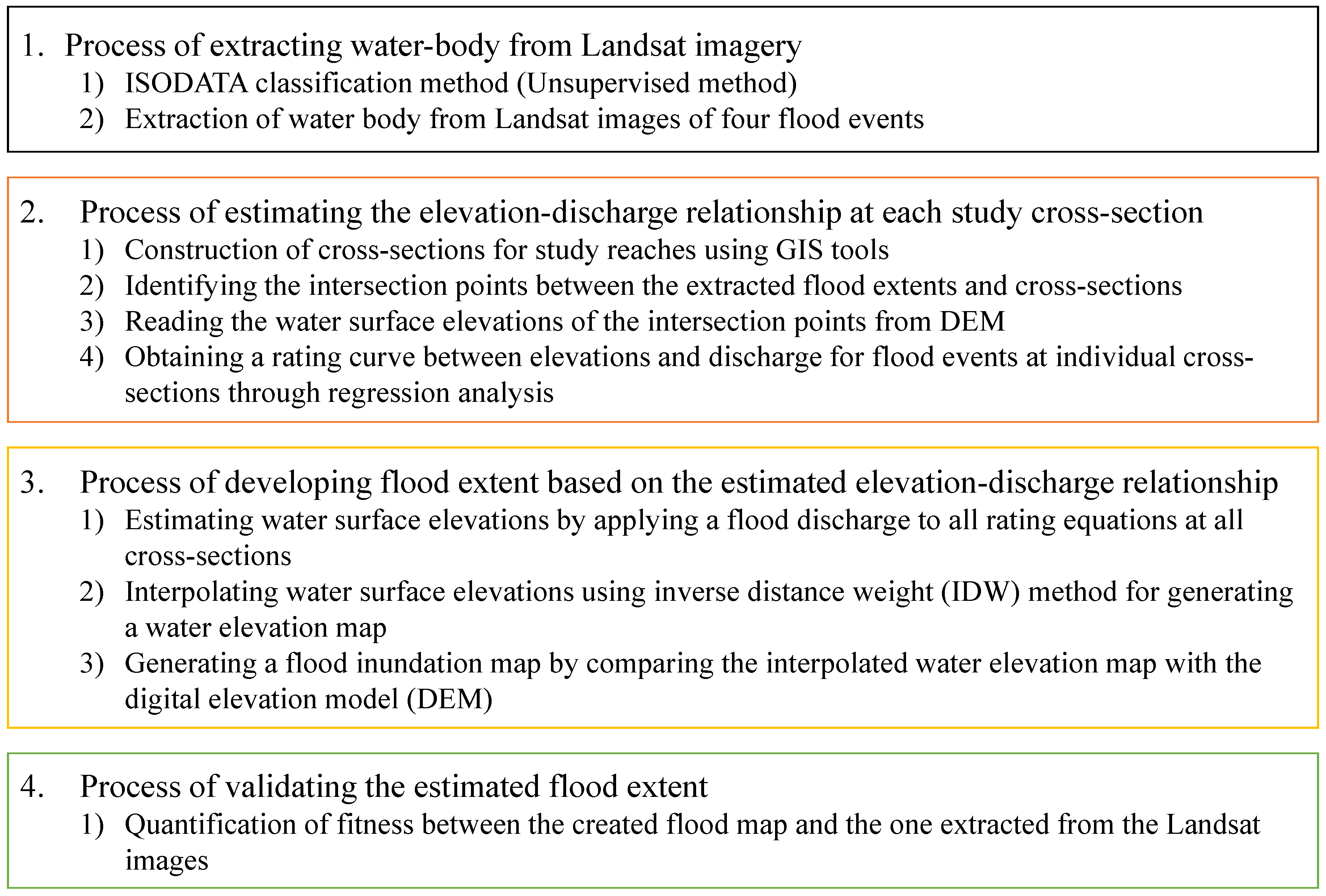
The methodology of this study is classified into the following four large categories (
Figure 1): (1) the process of extracting water bodies from Landsat imagery; (2) the process of estimating the elevation-discharge relationship at each study cross-section; (3) the process of developing flood extent based on the estimated elevation-discharge relationship; and (4) the process of validating the estimated flood extent.
2.1. Descriptions of Study Sites and Data
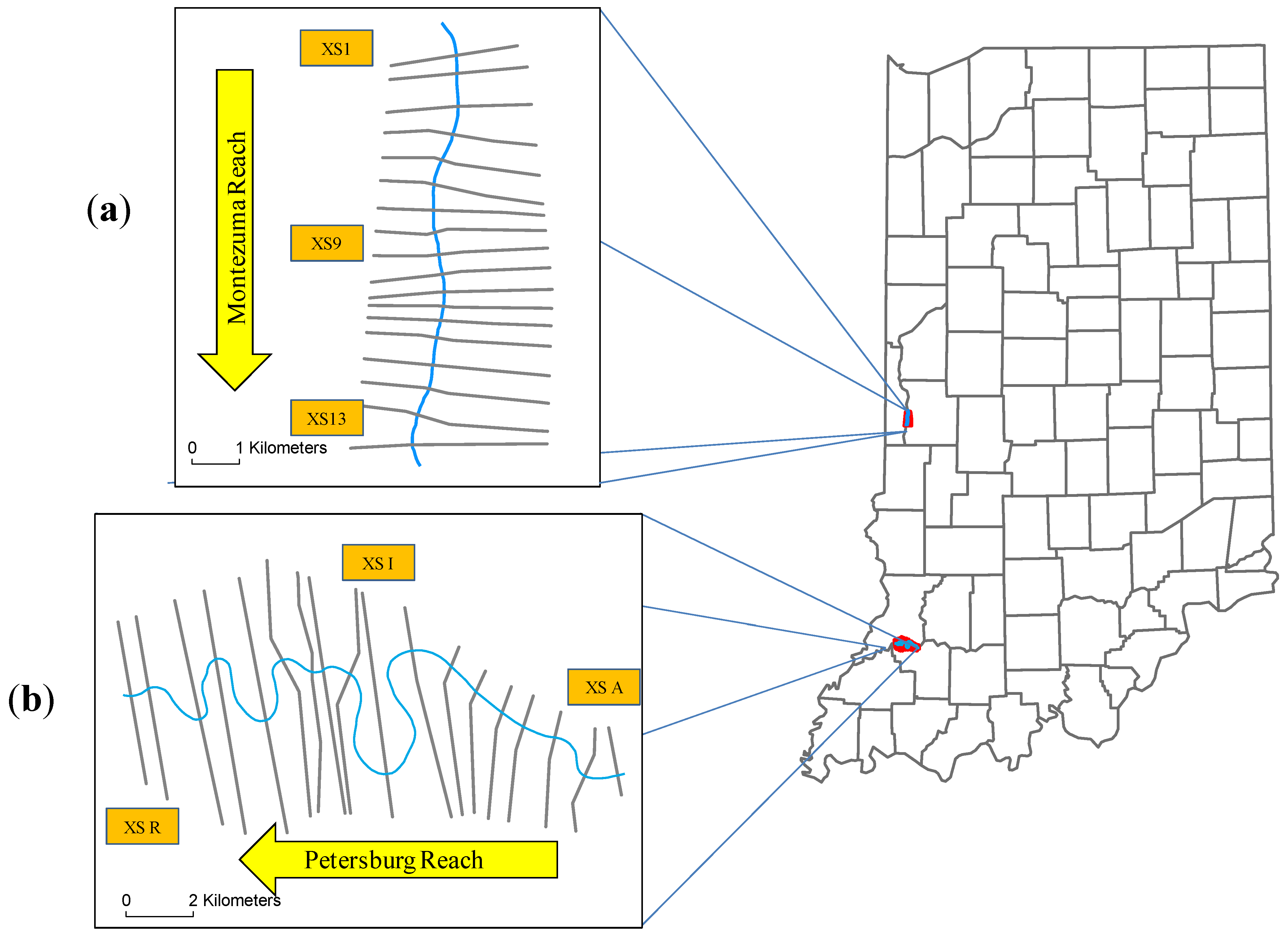
One reach of Wabash River, which drains to Mississippi River, Indiana, USA, and the other reach of White River, which drains to Wabash River were chosen as the study areas (
Figure 2). We call the first Montezuma Reach and the latter Petersburg Reach for the rest of this study for convenience because these reaches pass through the cities with the according names. These two reaches were chosen for the analysis for the following reasons: Satellite images taken by Landsat 5 Thematic Mapper (TM) imaging sensors are available from the USGS [
28] for most flood events that occurred after 2003 including the ones corresponding to the catastrophic flood that occurred in 2008 [
29]; Each reach has distinct topographic and geomorphic settings providing good test beds for comparison: The Montezuma Reach is relatively straight and is about 8km long. The Petersburg Reach is rather meandering and is about 28 km long. The number of cross-sections for flood elevation interpolation is 18 for both reaches.
Only cloud-free Landsat images based on which clear identification of the waterbody was possible were considered for this study. Four Landsat images were obtained and analyzed for both the Montezuma Reach and the Petersburg Reach. The times at which the images were taken and the corresponding flood discharge values are summarized in
Table 1.
Figure 2.
Study areas (a) the Montezuma reach and (b) the Petersburg reach (IN, USA).
Figure 2.
Study areas (a) the Montezuma reach and (b) the Petersburg reach (IN, USA).
Table 1.
The Landsat Imageries used in this study.
Table 1.
The Landsat Imageries used in this study.
| River Reach | Flood events | The available Landsat images | Peak flow |
|---|
| No. | Date | Discharge (m3/s) | Date | Discharge (m3/s) |
|---|
| Montezuma Reach | 1 | 10 April 2006 | 929 | 20 April 2006 | 1002 |
| 2 | 5 March 2007 | 1172 | 4 March 2007 | 1203 |
| 3 | 11 June 2008 | 1450 | 8 June 2008 | 2197 |
| 4 | 11 April 2009 | 1144 | 10 April 2009 | 1178 |
| Petersburg Reach | 1 | 5 March 2007 | 1260 | 4 March 2007 | 1286 |
| 2 | 22 April 2007 | 517 | 17 April 2007 | 991 |
| 3 | 11 June 2008 | 3645 | 12 June 2008 | 3738 |
| 4 | 3 July 2010 | 808 | 30 June 2010 | 1441 |
Stream flow data corresponding to each image was obtained from the USGS National Water Information System [
30]. The stream flow data of the USGS gage 03340500-Wabash River at Montezuma was chosen for the Montezuma Reach, and the stream flow data of the USGS gage 03374000-White River at Petersburg was chosen for the Petersburg Reach. DEM for both study reaches was obtained from the USGS Seamless Data Warehouse [
31]. The spatial resolution of DEM used in the analysis is 30 m. It should be noted that all data used in this study are in the public domain.
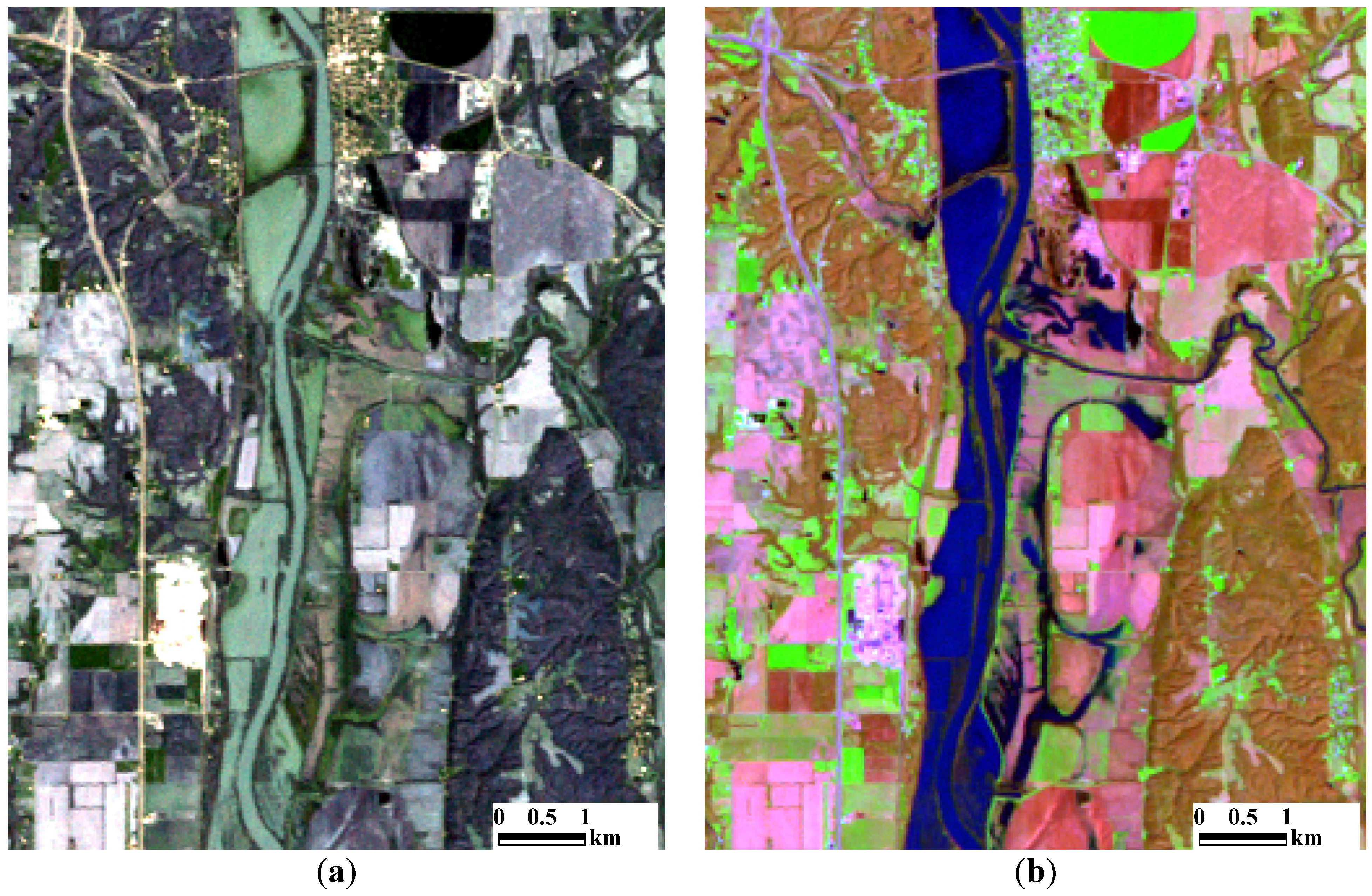
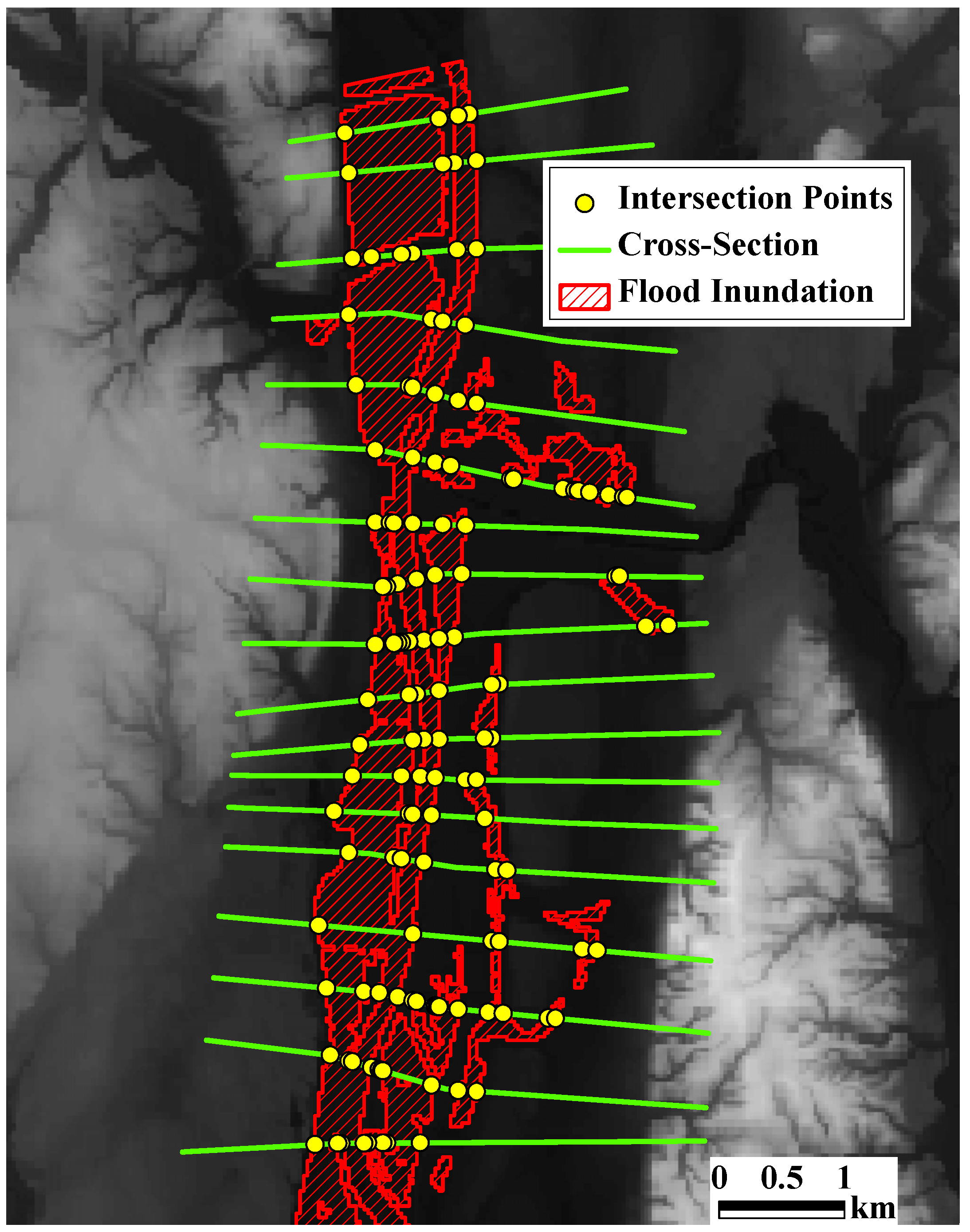
2.2. Extraction of Waterbody from Landsat Imagery
The process of extracting a waterbody from Landsat imagery was performed based on the image processing algorithm called ISODATA (Iterative Self-Organizing Data Analysis). In ISODATA, a number of points are randomly placed on the image. Then the pixels located within a given distance from the placed points are assumed to belong to the same cluster. In a next step, the variability of the pixel values within a cluster is calculated, which functions as a standard to further divide or merge the cluster in the next iteration. The iteration repeats until the specified criteria are met. In this study, ISODATA was applied to the imagery composed of the spectral bands 1, 4 and 7 of the Landsat data, which was classified into large clusters of 20 colors [
1]. This specific combination of the spectral bands was considered for the analysis because blue light (Band 1) penetrates clear water, near infrared (Band 4) is strongly absorbed in water, and mid infrared (Band 7) has spectral regions of absorption for water and reflectance for soil and rock [
32]. Then, the typical visible satellite images were overlaid, and the colors corresponding to the waterbody such as lakes, rivers, and reservoirs were chosen as the final waterbody. Lastly, the clusters classified into water were merged and exported into GIS format. The shades of the objects that were mistakenly classified as water were removed using the GIS tool.
2.3. Estimation of Elevation-Discharge Relationship
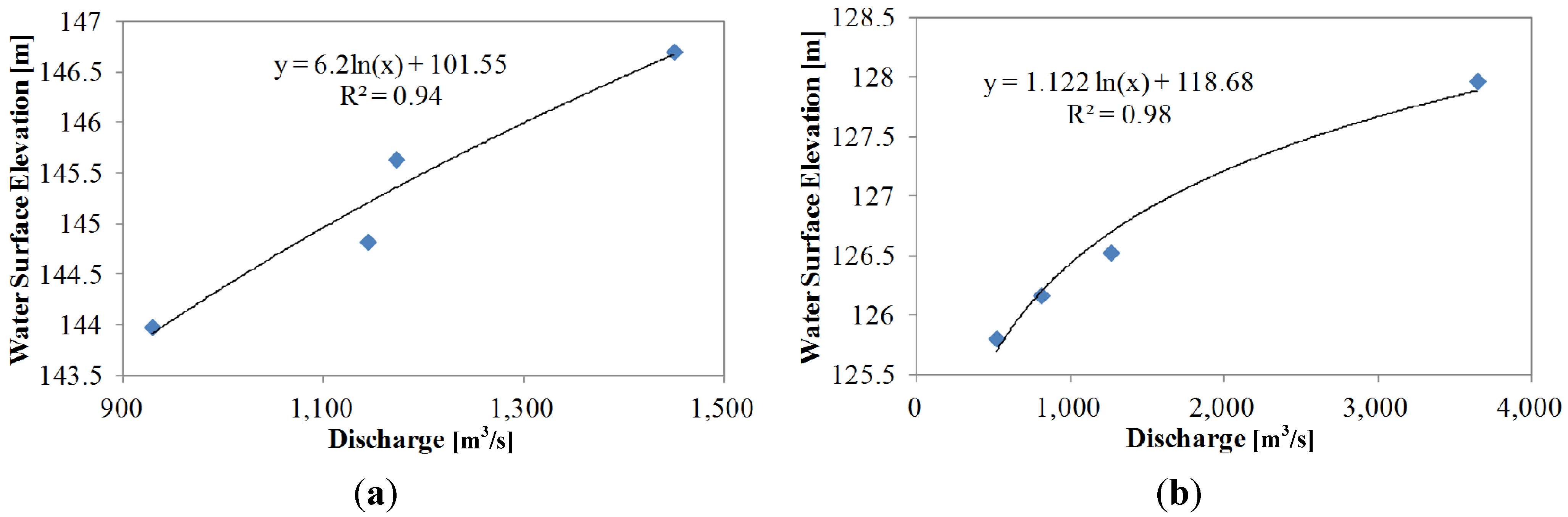
The elevation-discharge relationship was estimated using the following procedures: (1) digitizing cross-sections along the river reach using ArcGIS and HEC-GeoRAS; (2) identifying the intersections between the digitized cross-sections and waterbody boundary; (3) reading the elevation from DEM at the identified cross-section-waterbody intersections and determining a single representative elevation value. In this study, the mean of the spotted elevation values was taken as the flood elevation representing the cross section; (4) identifying the flow value corresponding to the time at which the Landsat imagery was taken. These values were obtained from the SGS National Water Information System; (5) repeating the processes from (1) to (4) for the Landsat images taken at different times to obtain more data points for the elevation-discharge relationship; (6) performing regression analysis to obtain the final form of the equation. Here, the shape of the regression was chosen from one of the following mathematical functions: logarithmic, linear, and second order polynomial. The shape that produced the least residuals, and thus the highest correlation, was chosen. In this study, both river reaches had 18 cross-sections and four Landsat data. Subsequently, elevation-discharge relationship with four data points was obtained for 18 river cross sections.
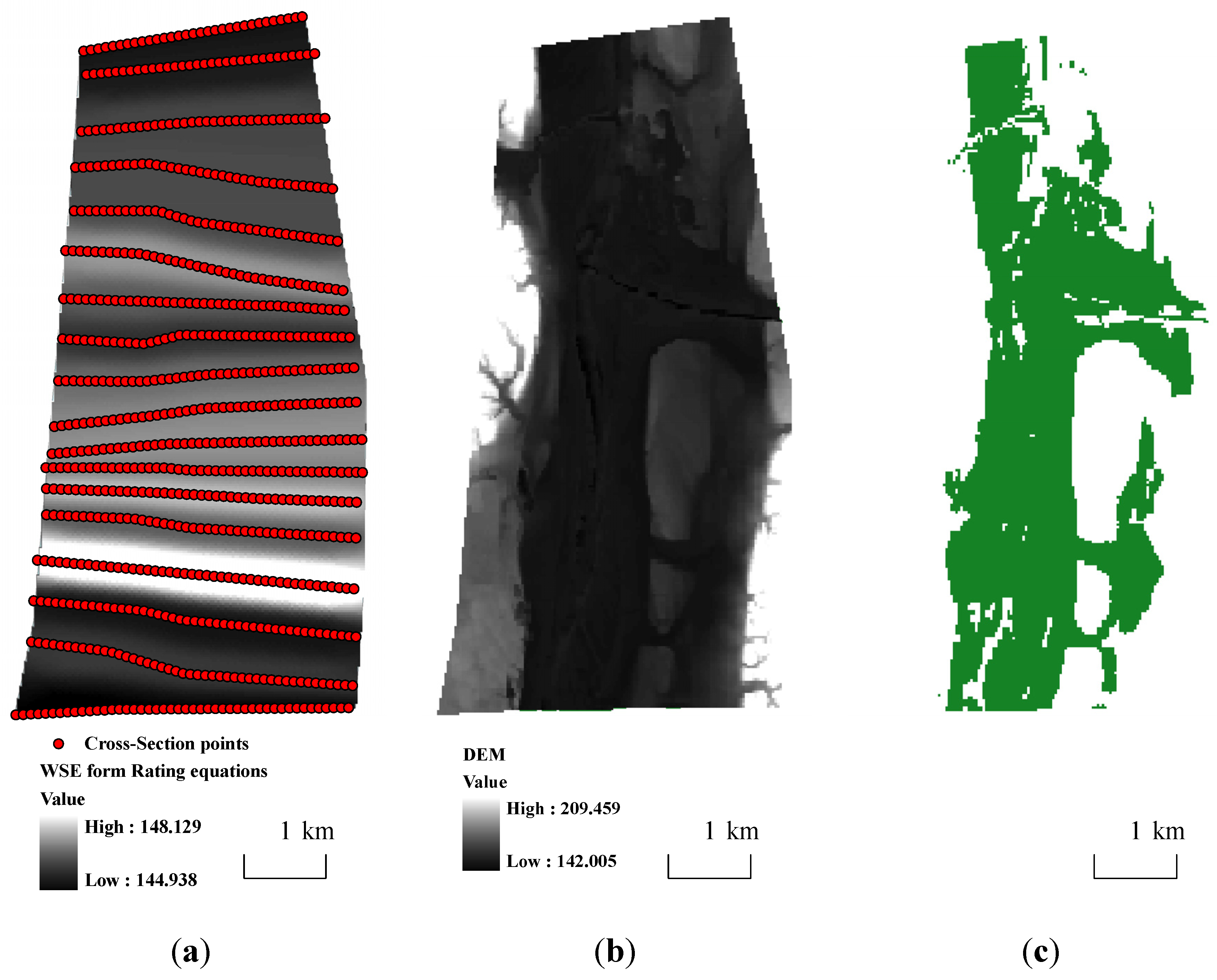
2.4. Flood Map Generation
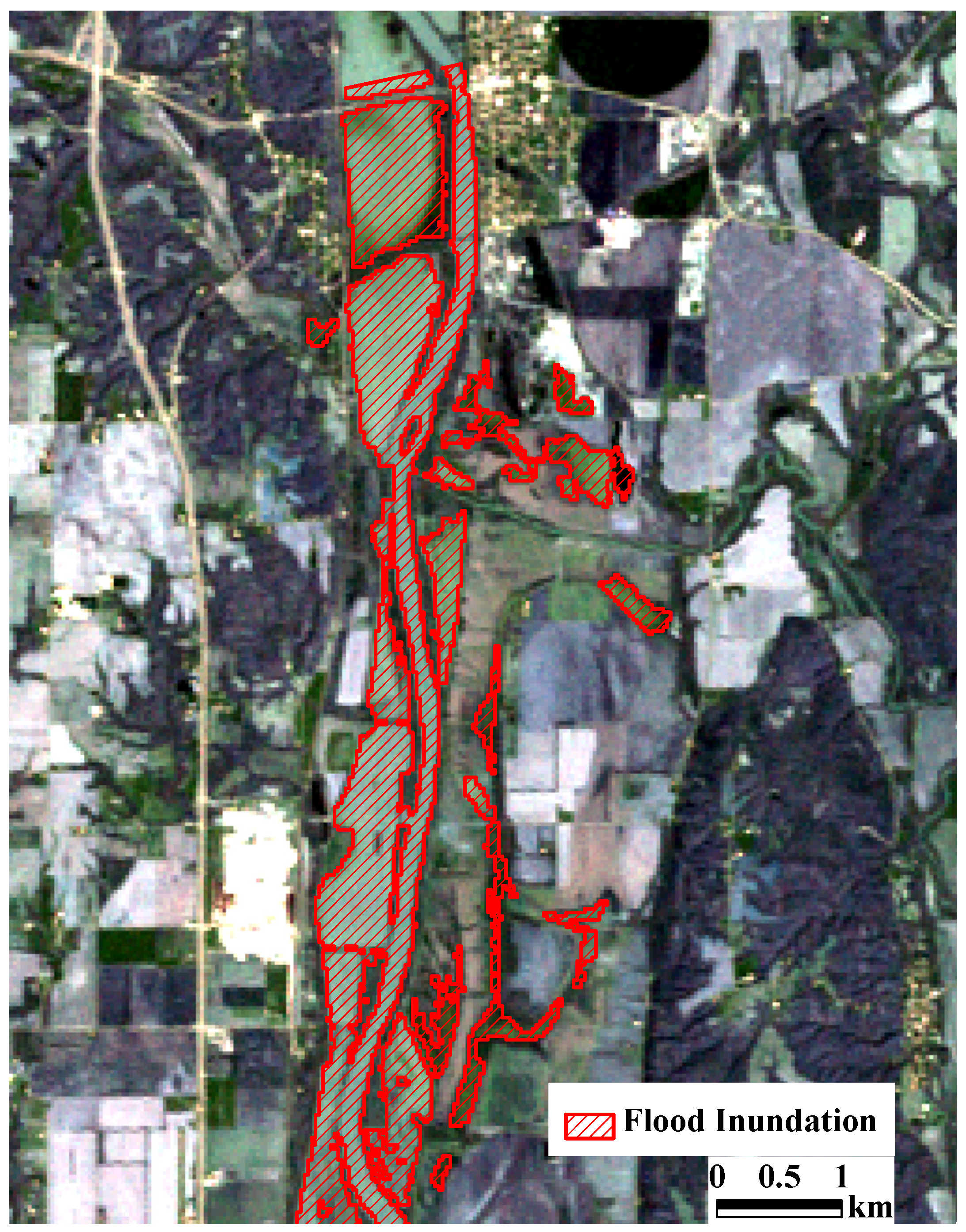
The process of flood map generation consists of the following steps: (1) identifying the flood elevation at each cross section; (2) generating the surface of flood elevation based on the identified flood elevation values at each cross section. Here, the method of inverse distance weight (IDW) was used for spatial interpolation; (3) generating a flood map using the raster subtraction geo-processing tool: Flood extent can be obtained by subtracting the surface elevation raster dataset (DEM) from the flood elevation raster dataset. Any raster cell for which the water surface elevation was greater than the surface elevation was considered as part of the flood extent.
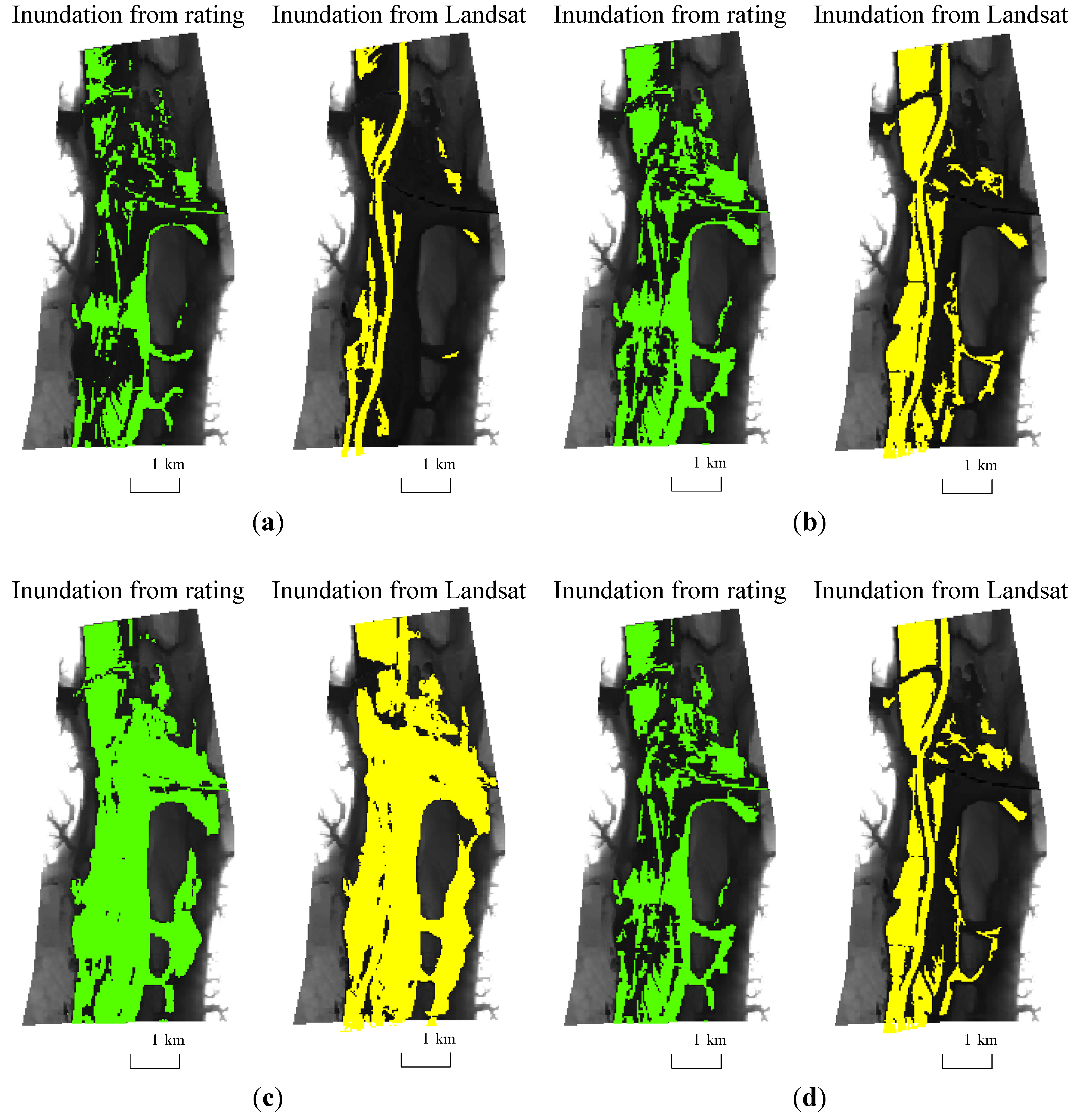
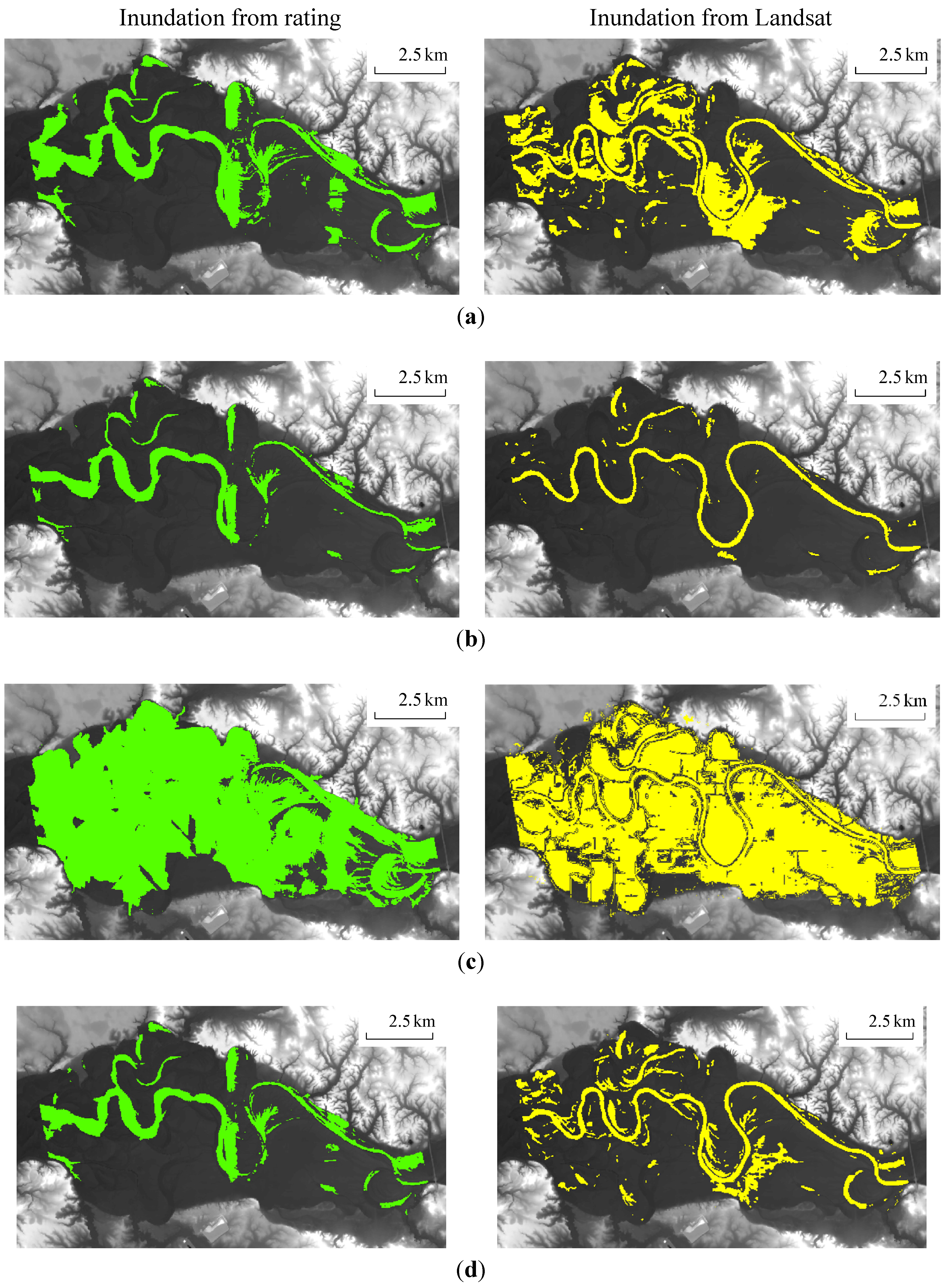
Flood inundation maps were created for the flood discharge values corresponding to satellite images, which were used to develop the same relationship. Then, the generated flood maps were compared to the same satellite images. The comparison method with which the satellite images were taken at the other flood events was originally considered, but this method was not possible due to shortage of the data. Therefore, it has to be noted that the result of this comparison does not validate or solidify the logic of the methodology suggested by this study. Instead, the result aims to reveal the limitations of the methodologies and to discuss uncertainties that can be induced while applying them.
The goodness of fit between the created flood map and the one extracted from the Landsat satellite images was assessed by the measure of relative error and F-statistics. Relative error (Equation 1) gives an indication of how well the inundation area extracted from Landsat imagery (
AL) compares to the inundation based on the estimated elevation-discharge relationship (
AR). The fact that the compared areas of the flood inundation are similar to each other does not necessarily mean that they are “geospatially similar.” For example, two flood inundations with exactly the same areas but with no overlapping portion will yield a relative error of 0 according to Equation 1. The use of F-statistics can resolve this issue. F-statistics (Equation 2) is defined as the ratio of the area of the overlapping portion of the two flood inundations to the area of both flood inundations projected on the map. It has been consistently used to compare the geospatial similarity of the mapped area over various studies [
33,
34,
35,
36].
where
Ao indicates the inundation area extracted from the Landsat images;
Ap refers to the predicted flood inundation area; and
Aop represents the intersection of
Ao and
Ap. High F-statistics indicates the goodness of fit between simulations and observations.
4. Discussion
The result of the comparison suggests that the flood extents delineated by the estimated elevation-discharge relationships can significantly differ from the ones directly extracted from the satellite images. This study attempted to newly develop a flood inundation map based on rating curves without any hydraulic model. Moreover, this approach can be useful to generate flood inundation maps in ungauged or data-poor regions where bathymetry of the river valley is unavailable. However, the fact that the estimated flood extent is based on the elevation-discharge relationship that is extracted from the satellite images being compared clearly reveals the limitation of the methodologies. Here, we focus on identifying the source of these limitations.
4.1. Limited Quantity of Satellite Images
The most important factor that limits this methodology is the limited quantity of satellite images. The satellite images used in this study were taken by Landsat 5 Thematic Mapper (TM) imaging sensors with the repeat cycle of 16 days. For the images to be used in the flood analysis, this repeat cycle has to coincide with the time close to flooding. Furthermore, the presence of clouds in the images, which has a high correlation with flow values, prevented the full use of the images obtained for the flooding periods. For this reason, only four data points could be used to obtain the elevation-discharge relationship. This prevented the dependable validation of the estimated rating equations developed at the cross section passing through the flow measuring point.
It also has to be noted that not all satellite images obtained and used for the analysis were used in this study. For example, a good number of images were available for low flow value, which displays the waterbody concentrated in the main channel, but these images were not considered for further detailed elevation-discharge relationship analysis because the resolution and the accuracy of the satellite imagery and DEM did not provide enough precision within the main channel along the cross-section.
In the future, it is expected that the use of visible/infra-red or radar data for classification of land use from satellite images will been introduced into the literature. Radar satellite images provide enormous potential for open water extraction due to their cloud penetration capacity. In this regard, radar satellite images will be appropriate to monitor spatio-temporal flood extents because flood inundation areas are often covered with heavy clouds [
37,
38].
4.2. Spatial Resolution of the Satellite Images and DEM
Both the Landsat imagery and the DEM that were used in this study have a horizontal resolution around 30 m. Even if ISODATA is able to extract the boundaries of a flood extent from an image perfectly, this level of coarse resolution of images can cause a significant amount of uncertainty in the spatial extent of the estimated flood extent boundaries. In the meantime, it also has to be considered that the each cell of DEM contains only a single value representing the elevation of around 900 m
2 of the cell area. For this reason, the flood elevation values used to develop the elevation-discharge relationship can contain a considerable amount of uncertainty. In addition to the horizontal resolution, vertical accuracy of DEM used in this study has the root mean square error of 2.44 m. This vertical error can directly be propagated to uncertainty in obtaining water surface elevation. Furthermore, it incorporates the uncertainties in the generation of the flood inundation area [
39,
40,
41].
4.3. Some Issues with Image Processing
Extraction of a waterbody from Landsat images can be conducted either with supervised or by unsupervised methods. For both of the methods, the person running the process has to make some crucial decisions or “train” the algorithm how to differentiate one class over others at the beginning or intermediate stages of the process. ISODATA used in this study is an unsupervised method for image processing, and the detailed information on a target land cover is not needed for classification. For this reason, ISODATA has frequently been used in waterbody classification [
42,
43]. However, unsupervised methods are limited by spectrally homogeneous groupings identified by the classification process. Moreover, while running ISODATA, the selection threshold, the number of iterations and the number of classification have to be given at the beginning of the processing. The extracted waterbody can differ significantly according to these initial parameters. In this study, the combination of Bands 1, 4, and 7 chosen on a subjective basis for image processing could induce uncertainties in the results. In addition, the change of waterbody transparency induced by natural factors, such as suspended sediments or other inorganic materials, can make the waterbody more turbid and less reflective misleading the identification algorithm. For a similar reason, the colors at the boundary of water bodies can be misclassified. For example, the wet ground surface can be considered as waterbody in the classification processes. Moreover, flooding water extracted from the Landsat images can be veiled by vegetation or urban constructions. The water bodies extracted in this study only reflect open water distribution (e.g.,
Figure 2 and
Figure 3).
4.4. Propagated Uncertainty in the Entire Processes
The above-mentioned limitations are sources of uncertainty for each step of this study. The final results obtained throughout many stages involve the uncertainties propagated from errors raised in each step. For example, an error in the waterbody extraction of the image processing propagates to the estimation of flood elevation with DEM, which involves horizontal and vertical errors. The regression method was used for the establishment of the relationship between discharge and flood estimation. Uncertainty in rating curves are also propagated to the generated flood inundation map.
5. Conclusions
Satellite images are widely adopted in various fields of natural sciences and engineering including meteorology, geology, forest sciences, and hydrology by providing useful geospatial information that would otherwise require significant amounts of effort for in-situ measurement and data integration. However, limitations of the analysis based on satellite images clearly exist due to the cursory and indirect nature of measurement compared to the ones performed on sites. The importance of this study is that (1) it introduces a new approach of flood inundation mapping based on satellite images and the elevation-discharge relationships that are extracted from the images; (2) it provides a measure of uncertainties expected while applying the suggested approach; and (3) it identifies the source of uncertainties requiring cautions during the application.
Even though the validation could not be fully performed due to the shortage of the satellite images, the suggested approach could develop a flood inundation map with a reasonable accuracy. The fact that the elevation-discharge relationship extracted from satellite images matches well with the “true” relationship at the USGS gauging stations proves this to a certain extent. The applicability of the methodology will be extended as more images become available, which can be either in the past or in the future. We also expect that the uncertainties to be induced by the factors stated above will significantly decrease as more satellite images become available.
The suggested flood mapping approach based on the elevation-discharge relationship requires the measured flow values at the points in time at which the satellite images were taken, which is not always possible in practice. For this reason, an approach to estimate the flow values based on satellite images to develop elevation-discharge relationship is also intriguing for future research.


