1. Introduction
Groundwater has been a primary source of potable and irrigation water for centuries. During the last 50 years, the soaring demand for freshwater has placed unprecedented stresses upon many aquifers throughout the world; many aquifers are now in overdraft. The projected growth in population combined with uncertainties associated with a changing climate will only aggravate this problem. A cost-effective advancement in groundwater/surface water management aimed at augmenting local water supplies is managed aquifer recharge (MAR), the practice of artificially recharging imported surface water, reclaimed (recycled) wastewater, or storm runoff into aquifers for storage and later extraction [
2,
3,
4].
For a MAR operation to be successful, a few challenges must be overcome. First, a source of recharge water must be found. Second, facilities, which can rapidly transfer water into aquifers, must be engineered. These include injection wells and spreading basins (recharge ponds), with both requiring periodic removal of accumulated clogging material to maintain recharge rates. Third, because the available water for the recharge operation can be of lesser quality than the local groundwater supply, there is the potential to degrade the existing aquifer. The introduction of salts, pathogens, disinfection by-products, and trace organic compounds such as pharmaceuticals, is a concern, especially when urban runoff or reclaimed wastewater is a large component of the source water for the operation [
4]. Lesser quality sources can become a larger portion of the recharge water at MAR operations because the availability of higher quality water such as imported water from remote watersheds is limited and may shrink due to shifts in climate and the diversion of this water to other uses such as maintaining riparian ecosystems (
i.e., loss of California State Water Project supplies to the delta smelt). Even in cases where the recharge water may be of a higher quality, it may have a different geochemical character (e.g., redox state) than the ambient groundwater and the potential exists for mobilization of intrinsic constituents, such as arsenic. For these reasons, it is vital to understand the fate and transport of potential contaminants near MAR sites. Only from this understanding can cost effective and appropriate regulations be developed.
Recent water quality studies near MAR operations have shown that many potential contaminants such as dissolved organic carbon (DOC), nitrate, some pharmaceuticals, and most pathogens are naturally removed or become inactive with time and distance in the subsurface (e.g., [
4,
5,
6,
7,
8,
9]). These water quality improvements, known as soil-aquifer treatment (SAT), are considered one of the benefits of MAR [
3,
4] and are generally observed soon after recharge, near the facility.
Despite these studies, water quality concerns still remain the focus of many regulations and an obstacle for the permitting of new MAR operations that include a reuse component (
i.e., reclaimed wastewater). For instance, MAR operations in California, USA, must conform to the state Drinking Water Program’s Groundwater Recharge Reuse Regulations, which require a subsurface retention time prior to its extraction for a potable supply that varies based on the level of pre-recharge treatment, in addition to a number of source water controls and how the travel times is being assessed [
10]. The required retention time varies from two to six months and must be verified using a tracer study.
1.1. Travel Time Estimates
Development of field methodologies to evaluate flow near MAR facilities is critical for the effective management of these operations where water quality assessment is warranted. The California Drinking Water Program’s Groundwater Recharge Reuse Regulations place a greater level of confidence on tracer data than on numerical models or Darcy flow calculations (see Table 2 in reference [
10]). Geochemical techniques provide a fundamental approach for investigating travel times, flow paths, recharge rates, and dispersivity in groundwater. Intrinsic environmental tracers such as Tritium/
3He (T/
3He) dating (e.g., [
11,
12]) are ideal for examining flow over spatial scales of kilometers and temporal scales of years to decades near MAR operations [
1,
13,
14]. Other environmental tracer dating techniques such as chlorofluorocarbons (CFCs) or sulfur hexafluoride (SF
6) are likely to be unreliable near MAR operations because non-atmospheric sources of these tracers may complicate the interpretation of apparent ages, especially when chlorinated reclaimed or potable water is being recharged (e.g., [
15,
16,
17]).
Because of the typical uncertainty associated with geochemical dating techniques (generally no better than ±2 years), these methods are not well suited for examining short-term transport specified by the Recharge Reuse Regulations in the state of California [
14]. Deliberate (
i.e., injected or applied) tracer experiments using gases such as SF
6 or noble gases (
i.e., He or Xe isotopes) have become acceptable methods for evaluating transport from recharge locations to wells over periods of weeks to a few years [
1,
10,
18,
19]. There is a long history of using SF
6 as a deliberate tracer starting with atmospheric experiments and expanding into aqueous systems initially by the gas exchange and oceanographic communities [
20,
21,
22,
23]. SF
6 can also be used as an intrinsic or environmental tracer for dating water in a similar fashion as CFCs [
17].
The scale of deliberate tracer experiments is defined by the quantity of water that can be “tagged” and the signal to noise ratio of the tracer being used. The three factors that often limit an experiment’s scale are: (1) identification of a tracer that does not adversely impact potable aquifers; (2) the cost of tracer; and (3) the ability to introduce a sufficient amount of tracer without significantly changing the buoyancy (or density) of the tagged water. The cost of the tracer can be a particular problem when large volumes of water (>10
5 m
3 or >80 AF) need to be tagged, as is often the case near MAR operations. As shown by the oceanographic community (e.g., [
20]), SF
6 can be used economically to tag large volumes of water.
There are cost advantages of using SF
6 over noble gas isotopes in terms of analysis; more SF
6 samples can be analyzed over a given period of time on less expensive equipment. However, it is a strong greenhouse gas and its emission is regulated in California. SF
6 is a synthetic gas used primarily in the electrical industry as a gas insulator and has been used as a tracer in the atmosphere and natural waters for more than two decades. It is an ideal tracer for the following reasons: (1) SF
6 is nontoxic [
24] and permission has been granted to use it as a tracer in potable aquifers in the southwestern USA and South Australia; (2) background concentrations of SF
6 in natural waters are extremely low (<0.05 pmol/L; 1 pmol = 10
−12 mole) because of its low solubility and low atmospheric mixing ratio (
ca. 8 pptv in 2014); (3) it can be measured precisely in water (±5% or better) over a concentration range of eight orders of magnitude (0.01 fmol/L to 1 nmol/L) using a gas chromatograph equipped with an electron capture detector [
25]; and (4) laboratory scale experiments have shown that breakthrough curves of SF
6 and bromide are identical in saturated porous media which contains either high contents of organic material or clays, demonstrating that SF
6 is not retarded (has a retardation factor of 1.0) [
26,
27].
SF
6 differs from ionic and dye tracers in that it is a gas and is easily lost from solution across the air—water interface to the atmosphere. It has often been used as a tracer for reaeration in surface water [
21,
22,
23,
28]. Thus, it is important to monitor the SF
6 concentrations in the recharge water to determine the amount of tracer lost due to gas exchange. This is especially true if the artificial recharge is taking place in a shallow river or spreading pond. Insufficient monitoring of the spatial variability of the tracer concentrations in the “spiked” surface water can lead to erroneous interpretations of travel times. Furthermore, laboratory column experiments have shown that SF
6 transport is slowed (retarded) when trapped air is contained within the porous media [
29,
30]. While there has been some evidence of gas tracer loss during recharge when a significant vadose zone is present, experiments conducted at three sites in California with a long history of fairly continuous recharge (OCWD, Orange County; Montebello Forebay, LA County; and El Rio, Ventura County) have shown that gas loss during percolation from spreading ponds is manageable if the tracer is introduced properly [
1,
13,
16,
18].
Fundamental questions concerning deliberate tracer experiments at MAR sites include: How general are the results? Can the results of an experiment performed several years in the past be used in the future? These questions arise because groundwater flow and travel times, e.g., to particular wells, should reflect hydrologic conditions at the time of the experiment such as recharge rates both at the MAR operation and surrounding area, pumping rates of nearby wells, and the regional hydraulic gradient. All of these are likely to change over time scales of months to years and imply that deliberate tracer results may not be similar year to year. For instance, long-term changes in the demographics and economics of an area could lead to changes in the locations and extraction/recharge rates from facilities. Furthermore, in areas with a Mediterranean climate such as Southern California, it is likely that recharge and groundwater production are out of phase, with the wet season having more recharge and less production. This should create seasonal variations in groundwater flow that should affect travel times, especially at shorter time scales (i.e., months).
In this paper, we discuss the results of two deliberate tracer experiments conducted at a spreading basin in Southern California that is operated by the Orange County Water District (OCWD), ten years apart to assess if travel times changed significantly over a decade.
1.2. Field Site
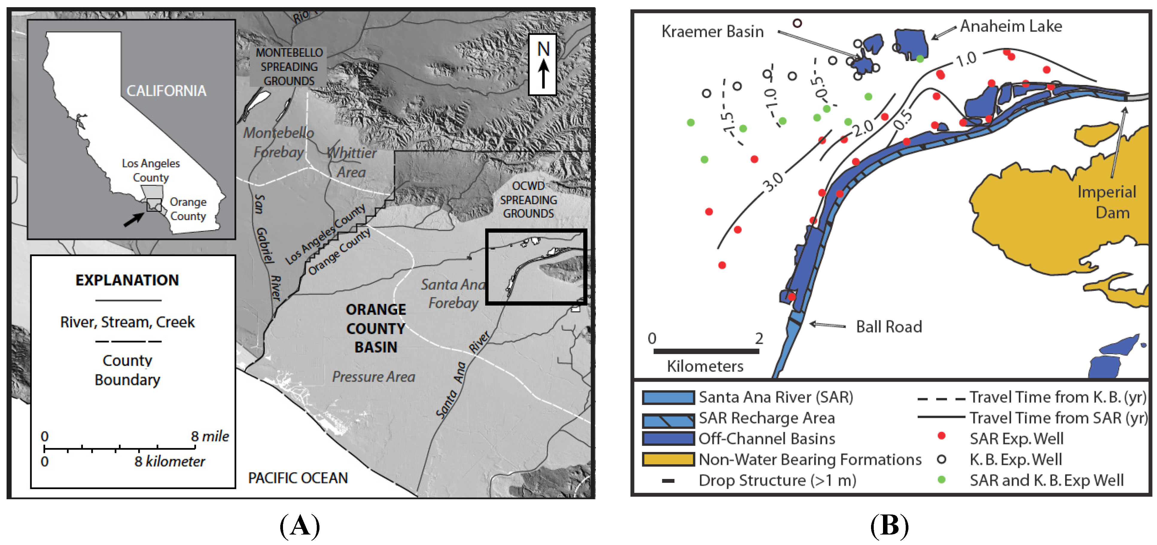
A 9-km section of the Santa Ana River (SAR) and a series of spreading basins, including Kraemer Basin and Anaheim Lake, located near Anaheim, California USA are used by the OCWD as principal recharge locations for the Orange County groundwater basin (
Figure 1 and
Figure 2). For more than 75 years, OCWD has been actively replenishing and managing the groundwater basin that supplies about 70% of the total water demand of approximately 2.4 million people and has been actively managing and replenishing the local groundwater basin. Currently, it operates more than 400 hectares of surface spreading facilities and recharges approximately 3.5 × 10
8 m
3 (2.8 × 10
5 AF; 10-year average between 2000 and 2010) per year [
31].
Figure 1.
Maps of the Orange County managed aquifer recharge (MAR) facilities. (
A) Topographic map of the field area including the location of Orange County Water District (OCWD) recharge basins based on data from the United States Geological Survey (USGS) 10-m National Elevation Dataset [
32]; (
B) Recharge occurs from the basins and from the Santa Ana River (SAR) between the Imperial Dam and Ball Road. The first arrival times of tracers determined in 1998 are contoured (modified from [
1]).
In January 2008, OCWD completed and began operating the Groundwater Replenishment System (GWRS), which is the world’s largest wastewater purification system for indirect potable reuse [
33]. The system produces up to 2.43 × 10
5 m
3 (197 AF) of high quality reclaimed water each day using a three-step advanced treatment process that consists of microfiltration, reverse osmosis, and ultraviolet light disinfection with hydrogen peroxide advanced oxidation. A variable portion of the reclaimed water is pumped about 20 km to the MAR facilities and is recharged through Kraemer and other permitted nearby basins to replenish the groundwater.
Detailed investigations of the groundwater flow were conducted in the late 1990s using a variety of techniques including T/
3He dating and deliberate tracer experiments at Anaheim Lake, Kraemer Basin, and the SAR [
1,
34]. The January 08 SF
6 experiment was required by state regulators because of the use of Kraemer Basin for GWRS water recharge and to determine if travel times near Kraemer Basin were similar to those determined a decade earlier during the October 1998 Xe isotope tracer experiment.
2. Materials and Methods
The methodology of Clark
et al. [
1] was used during the January 2008 Kraemer Basin deliberate tracer experiment and is outlined below. At the time of the tracer injection, the basin contained approximately 1.4 × 10 m
5 (2000 AF) of water. The volume increased during the experiment and by the end, the pond contained about 2.1 × 10 m
5 (3000 AF). The study began on 17 January 2008 (defined as day 0) when 99.8% pure SF
6 gas tracer was carefully injected into Kraemer Basin over a period of about 1 hour by bubbling the tracer through a submerged diffusion stone at a rate of about 40 mL/min at two locations ~10 m offshore (
Figure 2C). This injection technique was repeated twice more, on day 8 and 11. During each injection, SF
6 formed a rising bubble plume that only partially dissolved in the water column (bubbles could be seen bursting at the surface); therefore, an unknown quantity of tracer was released into the recharge water. Previously, it was estimated that less than 5% of the bubbled gas dissolves [
14,
18,
19,
34].
Figure 2.
Maps of the Orange County MAR facilities. (A) Photograph of the basin looking from the northern shore to the south towards the boat ramp. The inserted photo shows one of the fixed buoys; (B) Detailed map of the January 2008 field area showing the sampled wells and principle recharge areas. At the start of the experiment, neither Miller nor La Jolla Basins were recharging the aquifer. For reference, the north-south 57 freeway and the east-west 91 highway have been included. The black dashed arrows represent the northern and southern flow lines, the solid purple and dashed/dotted green contours represent, respectively, the and November 1998 and June 2008 piezometric surfaces; (C) Detail of Kraemer Basin at the time of the 2008 tracer injection showing where tracer was introduced and sampled.
Because it is vital to know the initial dissolved tracer concentration, SF
6 surveys of Kraemer Basin water were conducted on days 1, 3, 5, 8, 9, 11, 12, 14, 18, and 22. During each survey, surface (~1 m below the pond’s surface) and bottom (~1 m above sediment) samples were collected from five stations evenly distributed throughout the basin and marked with fixed buoys (
Figure 2A,C). Approximately 2–3 mL samples were collected in Vacutainers™ in triplicate for storage and later analysis. Vacutainers™ are convenient storage and reaction containers that are commercially available. Surveys were conducted until the mean SF
6 concentration decreased to approximately the detection limit. Following the tracer injection, well samples were collected for a period of one year by personnel from OCWD in Vacutainers™ and sent to UCSB for analyses, which generally occurred within two weeks of collection. The frequency of sampling was adjusted for each well based on the results of recent sampling.
All SF
6 samples were analyzed using a headspace method similar to that described by [
1]. In the field, pre-weighed 10 mL Vacutainers™ were partially filled (2–5 mL of water). In the laboratory, these containers were weighed (to determine the sample weight) and carefully filled with ultra-high purity nitrogen gas (so that the final pressure was equal to about 1 atmosphere). After a brief shaking to mix the headspace, this gas was injected through a column of Mg(ClO
4)
2 (to remove water vapor) into a small sample loop of known volume (about 1.5 mL). Subsequently, the gas in the sample loop was flushed into a gas chromatograph equipped with an electron capture detector with ultra-high purity nitrogen carrier gas. SF
6 was separated from other gases with a molecular sieve 5a column held at room temperature. The detector response was determined by running gas standards purchased from and certified by Scott-Marrin, Inc. (Riverside, CA, USA). The detection limit of this method is about 0.05 pmol/L, three orders of magnitude lower than the mean pond concentration (see below). Error on duplicate Vacutainer™ measurements was typically better than ±10% but not as good as the ±5% reported for the syringe headspace method [
25].
At each well, arrival times of tracer can be determined by evaluating breakthrough curves, which are plots of concentration
versus time. In homogenous aquifers—sand boxes, the initial and mean arrival (center of mass or COM) times of tracer at narrow-screened monitoring wells represent, respectively, the fastest and mean flow paths in the aquifer. In heterogeneous aquifers with preferential flow paths tracer breakthrough curves are more complicated, often showing multiple peaks [
1,
14]. Tailing is also evident on breakthrough curves and can represent the tracer reaching the well by slower flow paths, back diffusion out of lower permeability strata, non-ideal tracer input function, or retardation, which in the case of gas tracers can be due to trapped gas [
29,
30]. As discussed by Becker
et al. [
35], sampling biases can result in moderate and hard to quantify travel time errors. These biases are often caused by infrequent sampling due to budget limitation.
3. Results and Discussion
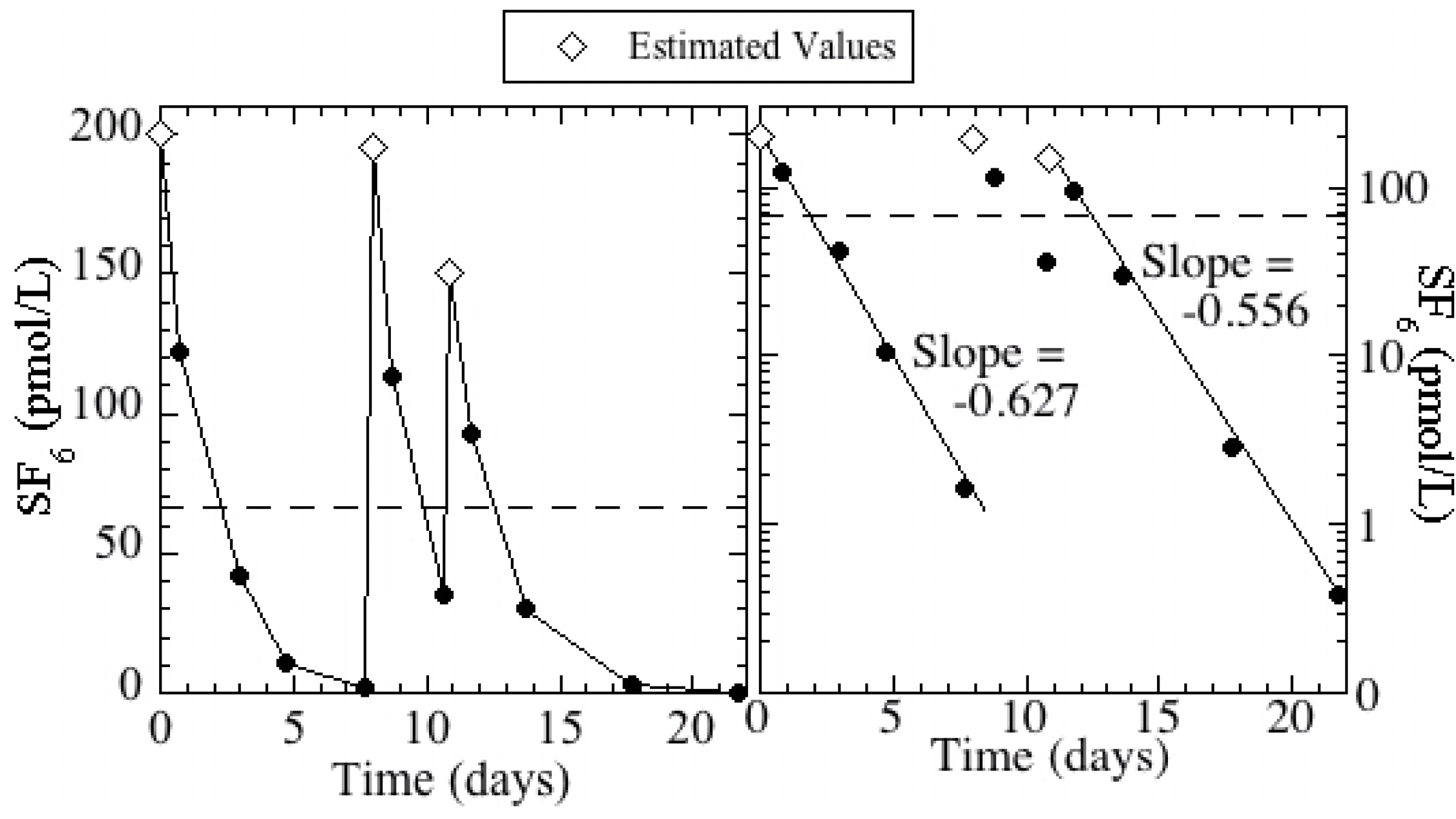
Mean basin concentrations of SF
6 tracer determined for each survey ranged between about 0.4 pmol/L (day 22) and 120 pmol/L (day 9); the daily infiltration rate varied between 1.7 m
3/s (day 20) and 2.2 m
3/s (days 6 and 7) and averaged 1.95 ± 0.15 m
3/s (68.9 ± 5.3 cfs). The basin concentrations were the highest following the injections and decreased exponentially due to recharge and gas loss across the air-water interface (
Figure 3). The rate of loss was slightly greater during the first week than during the second, most likely due to the progressive deepening of the basin as it was filling with recharge water. This would increase the mean residence time of water in the basin and decrease the gas exchange loss.
Figure 3.
SF6 concentrations in Kraemer Basin during the injections and subsequent monitoring periods. Injections occurred on days 0, 8, and 11; estimated basin concentrations are plotted for these days. The dashed line represents the 14-day flow weighted mean concentration (66 pmol/L) during the defined injection period.
The tracer injection period was defined as the first 14 days (between January 17 and 31) when 96% of the total mass injected percolated into the ground and the flow-weighted mean SF
6 concentration was 66 pmol/L. It is important to note that the basin concentration decreased below 10% of the mean for 2 days (days 6 and 7) in the middle of the injection period (
Figure 3). This complexity in the basin concentration is apparent in the breakthrough at monitoring well KBS-3/1, which displays two peaks (
Figure 4B).
Although the water level contours represent different seasons and therefore different water use times in terms of the domestic landscape irrigation cycle, they are sub-parallel indicating that the location of recharge and pumping remained similar between experiments (
Figure 2B). However, the hydraulic gradient west-southwest of Kraemer Basin was ~50% steeper in November 1998 (~0.0064) than June 2008 (~0.0042). Furthermore, the absolute elevation of the piezometric surface was about 5 m higher in June. These changes most likely reflect seasonality rather than long-term use patterns. The June survey occurred near the beginning of heavy domestic landscape irrigation while the November survey reflects water levels at the end of this irrigation period.
Groundwater samples were collected at 28 monitoring points (at 17 well sites, three of which were multi-level: AMD-10, AMD-11, AMD-12;
Figure 2B), with sufficient frequency to construct tracer breakthrough curves (
Figure 4). Tracer was detected at twelve wells down gradient (to the west) of Kraemer Basin (
Table 1). As was observed during the October 1998 Xe isotope tracer study [
1,
33], detections progress systematically to the west along two flow paths that follow the local hydraulic gradient: the northern path of KBS-3/1, AM-7, AMD-12/1, AM-48, and AM-8; and the southern path of KBS-1/1, KB-1, AMD-11/1, AM-10, AM-9, and AM-14 (
Figure 2B). The one exception is the tracer’s first arrival was essentially the same at the deeper screened AMD-11/1 and AM-10 even though AMD-11/1 was more distant. This implies that depth as well as distance is important when considering travel times and that the first arrival is a difficult parameter to interpret. Interestingly, the arrival of the COM followed the distance trend with it arriving at AM-10 prior to AMD-11/1.
Figure 4.
Breakthrough curves at representative wells. Wells found along, respectively, the southern (A, C, E) and northern (B, D, F) flow paths are displayed on the left and right. The mean pond concentration was 66 pmol/L and non-detections (<0.05 pmol/L) have been plotted as “0 pmol/L”. Please note that the scale on the y-axes (concentration) differs.
Table 1.
Summary of travel times during the Oct-98
136Xe and Jan-08 SF
6 tracer experiments from Kraemer Basin. The Oct-98 Xe isotope data is from [
33]. The distance was measured from the basin’s shoreline directly to the well. This is the shortest distance and does not necessarily represent the flow path length. Travel times are in weeks.
Table 1.
Summary of travel times during the Oct-98 136Xe and Jan-08 SF6 tracer experiments from Kraemer Basin. The Oct-98 Xe isotope data is from [33]. The distance was measured from the basin’s shoreline directly to the well. This is the shortest distance and does not necessarily represent the flow path length. Travel times are in weeks.
| Well | Distance (m) | Screen Interval (m msl)* | Jan-08 SF6 | Oct-98 136Xe |
|---|
| First Detect | Peak | COM | First Detect | Peak | COM |
|---|
| Northern Flow Path | | | | | | |
| KBS-3/1 | <100 | 44 to 41 | 2.7 | 4.7 | 5.6 | <1.4 | <1.4 | † |
| AM-7 | 130 | 1 to −4 | 10.6 | 22.9 | 25.4 | 8.3 | 15.1 | 15.3 |
| AMD-12/1 | 525 | −36 to −42 | 16.6 | 22.9 | 30.5 | — | — | — |
| AM-48 | 1250 | −20 to −29 | <16.6 | 18.7 | 25.7 | — | — | — |
| AM-8 | 1250 | −26 to −31 | 20.9 | — | 37.1 † | 17.7 | 23.0 | 38.3 |
| Southern Flow Path | | | | | | |
| KBS-1/1 | <100 | 4 to 1 | <1.6 | <1.6 | † | 1.4 | 1.4 | — |
| KB1 | <100 | 13 to 7 | 1.6 | 3.6 | 6.0 | 2.6 | 2.3 | 3.7 |
| AM-10 | 1000 | −3 to −8 | 6.6 | 20.9 | 23.8 | 15.1 | 23.0 | 28.4 |
| AMD-11/1 | 1260 | −91 to −97 | 6.7 | 29.1 | >28* | — | — | — |
| AM-9 | 1840 | −26 to −31 | 15.7 | 26.6 | 33.8 | 26.4 | 39.7 | 50.6 |
| AM-14 | 2630 | −32 to −38 | 37.7 | 37.7 | † | 45.8 | — | 67.9 |
At relatively shallow wells (<65 m to the screen top) near the basin (KB-1, KBS-1, KBS-3), tracer was first detected <1 to 3 weeks after the beginning of the injection period. This was not the case at another nearby well, AMD-10, where the tracer was never detected in the five zones sampled, which have screen tops between 90 and 285 m below ground surface. This is in agreement with the October 1998 experiment [
1,
33], which showed that these zones are hydraulically connected with Anaheim Lake (
Figure 1 and
Figure 2B), a recharge basin up gradient (to the east) of Kraemer Basin, once again indicating the importance of depth to the flow field.
The influence of depth is best explained by the complicated local hydrostratigraphy. The water recharged from the basins is not flowing through a sand box, rather it flows through conductive layer between confining and semi-confining layers [
1,
33,
36]. This complicated hydrostratigraphy also helps to explain the reversal of arrival time (first
vs. COM) at AM-10 and AMD-11/1 and points to a potential problem of using a tracer with a large signal to noise ratio. There is no doubt that the first arrival time is poorly defined: the arrival is defined by the first detection of the tracer and therefore is defined by which tracer is being used and how good the analytical system is. Therefore the signal to noise ratio of the tracer is vital for determining this arrival time and not the local hydrology. It may make sense in the future to define this arrival time with C/C
0, where C
0 could be either the initial concentration in the recharge water or the local peak concentration. We believe that the former makes more sense because in is likely that the local peak concentration cannot capture unless continuous sampling is employed.
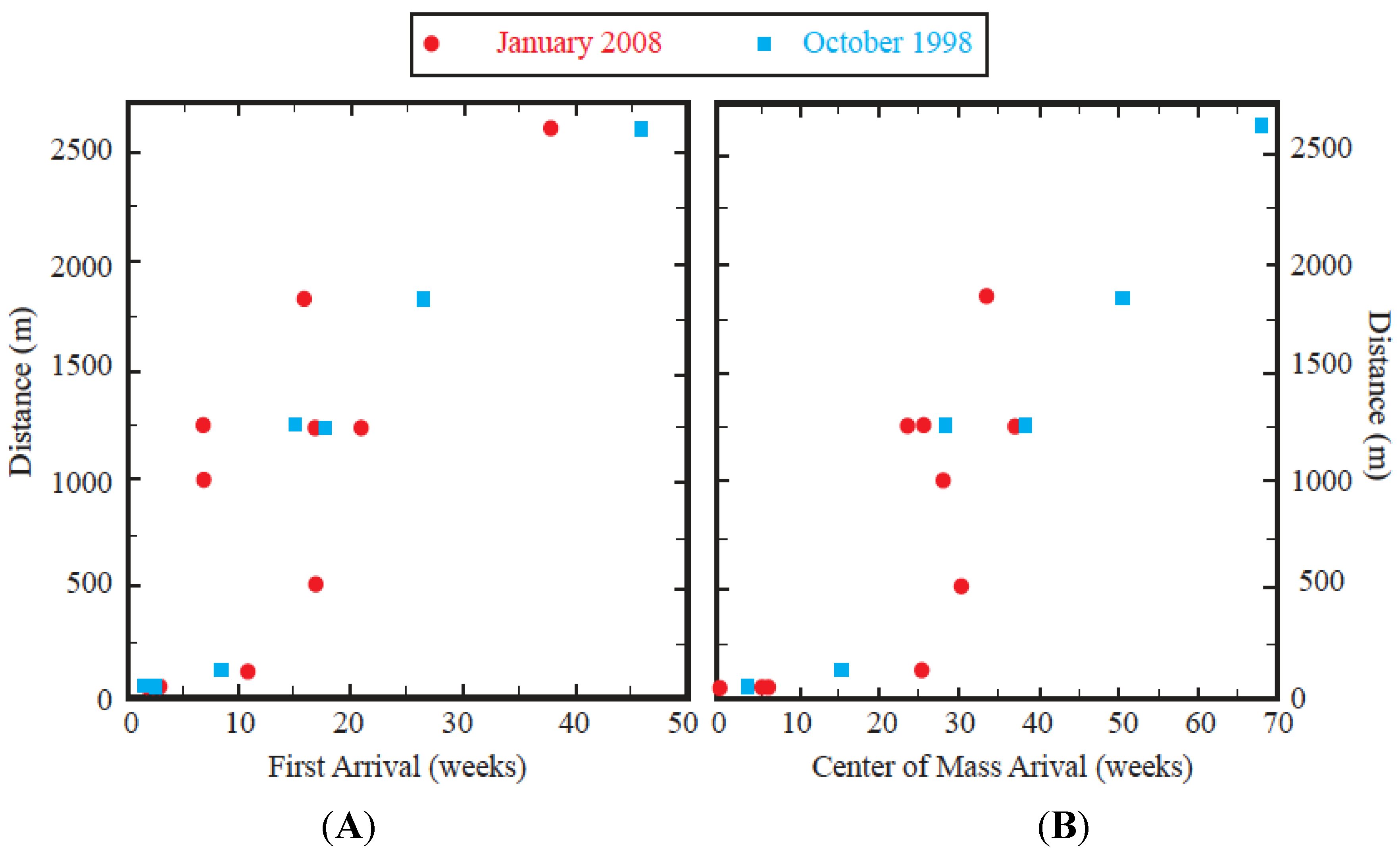
The travel times of the leading edge of the tracer arrival, which is defined by the first detection, were very similar (within three weeks) at six of the nine wells monitored during both the 2008 and 1998 experiments (
Figure 5A;
Table 1). The mean observed velocity of the leading edge was about 60 m/week (3 km/year). The exceptions were the three most distant wells along the southern flow path, AM-9, AM-10, and AM-14. During the 2008 experiment, the tracer arrival was traveling about 50% faster and, therefore, earlier detections were observed at these wells.
Figure 5.
Comparison between the arrival times and distance from the January 2008 and October 1998 tracer experiments. (
A) First arrival and (
B) COM. Note the change of scale on the x-axis. During the January 2008 experiment, COM arrivals could not be calculated at all wells because of incomplete breakthroughs (see
Table 1).
Monitoring wells AM-8, AM-48, AM-48A, and AM-49 are located along the northern flow path approximately the same distance down gradient. However, the screen depth of these wells differs. Tracer was not detected at the relatively shallow wells, AM-48A and AM-49 (screen depths between 20 and 30 m msl) while it was detected at the deep wells, AM-8 and AM-48 (screen depths between −20 and −31 m msl). This implies that the tracer had migrated vertically downward beneath the water table and was traveling through deep layers, with the shallow layers recharged by other sources, such as the nearby La Jolla Basin (
Figure 2B). The movement of the COM was also very similar during two experiments (
Figure 5B) and traveled with a velocity of about 40 m/week (2 km/year).


