Next Article in Journal / Special Issue
Managed Aquifer Recharge (MAR) Economics for Wastewater Reuse in Low Population Wadi Communities, Kingdom of Saudi Arabia
Previous Article in Journal
Attribution of Decadal-Scale Lake-Level Trends in the Michigan-Huron System
Previous Article in Special Issue
Economic Assessment of Opportunities for Managed Aquifer Recharge Techniques in Spain Using an Advanced Geographic Information System (GIS)
 
 
Correction published on 17 December 2014, see Water 2014, 6(12), 3957-3959.
Article

A System Dynamics Model to Conserve Arid Region Water Resources through Aquifer Storage and Recovery in Conjunction with a Dam

1
Department of Geoscience, Faculty of Science, University of Calgary, 2500 University Dr. NW, Calgary T2N 1N4, Canada
2
Department of Bioresource Engineering, Faculty of Agricultural and Environmental Sciences, Macdonald Campus of McGill University, 21111 Lakeshore Road, Sainte-Anne-de-Bellevue, QC H9X 3V9, Canada
3
Department of Civil Engineering and Applied Mechanics, Faculty of Engineering, McGill University, 3450 University Street, Montreal H3A 0C3, Canada
*
Author to whom correspondence should be addressed.
Water 2014, 6(8), 2300-2321; https://doi.org/10.3390/w6082300
Submission received: 15 May 2014 / Revised: 22 July 2014 / Accepted: 29 July 2014 / Published: 7 August 2014
(This article belongs to the Special Issue Policy and Economics of Managed Aquifer Recharge and Water Banking)

Abstract

:
Groundwater depletion poses a significant threat in arid and semi-arid areas where rivers are usually ephemeral and groundwater is the major source of water. The present study investigated whether an effective water resources management strategy, capable of minimizing evaporative water losses and groundwater depletion while providing water for expanded agricultural activities, can be achieved through aquifer storage and recovery (ASR) implemented in conjunction with water storage in an ephemeral river. A regional development modeling framework, including both ASR and a dam design developed through system dynamics modeling, was validated using a case study for the Sirik region of Iran. The system dynamics model of groundwater flow and the comprehensive system dynamics model developed in this study showed that ASR was a beneficial strategy for the region’s farmers and the groundwater system, since the rate of groundwater depletion declined significantly (from 14.5 meters per 40 years to three meters over the same period). Furthermore, evaporation from the reservoir decreased by 50 million cubic meters over the simulation period. It was concluded that the proposed system dynamics model is an effective tool in helping to conserve water resources and reduce depletion in arid regions and semi-arid areas.

Graphical Abstract

1. Introduction

Groundwater extraction has enabled significant social development and economic growth, enhanced food security and alleviated drought in many of the world’s farming regions [1]. However, if groundwater abstraction exceeds groundwater recharge or decreased baseflow, persistent groundwater depletion or overexploitation problems can occur [2,3]. Groundwater depletion is a significant threat in arid and semi-arid areas, where rivers are usually ephemeral and groundwater is the primary source of water. Consequently, in many arid countries, dams are built on ephemeral rivers to provide farmers with an expanded and reliable source of water. However, the major disadvantages of dams in arid regions are the high evaporation loss from reservoirs and water quality degradation.
An alternative to constructing dams is recharge enhancement [4], a technique used to increase groundwater availability. One well-known recharge enhancement technique is the engineered system of aquifer storage and recovery (ASR), whereby surface water is moved to aquifers via infiltration, seepage or deep injection wells and serves to bolster groundwater resources. This water can later be recovered for reuse by conventional pumping. The technique was first implemented in 1957 to inject potable water into saline aquifers [5,6].
Given increasing water demand, stresses on supply and wet versus dry season water imbalances, artificial recharge is likely to become an important component of water projects in arid and semiarid regions [7]. Aquifers offer significant opportunities for underground water storage, reducing the need of high-cost surface reservoirs and storage tanks. Applying ASR techniques can also act to restore a depleted aquifer’s functionality [8]. Moreover, ASR can improve agricultural water security, thus improving the livelihood of farmers and providing economic, social and environmental benefits.
In terms of economic benefits, ASR has direct, as well as indirect financial benefits. The costs involved in ASR projects depend on several variables, including location, land prices, method of recharge, geological conditions, design of the entire holistic system, construction costs and initial water quality [9,10]. For two such projects in Australia, the costs of recharge per million liters were 625 USD and 2,000 USD [5,11]. In addition, ASR increases agricultural productivity, which, in turn, improves farmers’ livelihood and provides direct benefits, not only at the economic level, but also at the social and cultural levels. A cost benefit analysis developed for a case study in southwest Iran found a 1:1.32 ratio of project investments to agricultural profits, with an estimated payback period of three years [12].
In basins approaching full development of water resources, optimal beneficial use can be achieved by conjunctive use, which involves coordinated and planned operation of both surface water and groundwater development. The concept of conjunctive use of surface water and groundwater is based on surface reservoir impounding stream-flow, which is then transferred at an optimum rate to groundwater storage. Surface storage in reservoirs behind dams supplies most of the annual water requirements, while groundwater storage can be retained primarily for cyclic storage to cover years of subnormal precipitation [13].
There are some successful examples of conjunctive water resources management around the world, such as the elaborate institutional arrangements for conjunctive use and groundwater management in southern California that have been in place since the 1950s [14]. Kern Water Bank (KWB) in California is another successful example. The KWB stores excess water supplies that are available when rainfall or runoff is plentiful by recharging that water through shallow ponds into an aquifer. The stored water is then recovered in times of need by pumping it out with wells [15]. In some cases, treated sewage effluent has been used as the source of water. For example, sewage reclaimed water from an advanced treatment facility is recharged in the wells of the hydraulic barrier constructed to protect the Los Angeles coastal aquifer from seawater intrusion in southern California. Similarly, in the Dan region in Israel, treated sewage effluent from the metropolitan area of Tel Aviv is recharged in sand dunes and then subsequently pumped for various uses [16].
The objective of this study was to determine if ASR, in conjunction with water storage on an ephemeral river, can be an effective water resource management strategy, minimizing evaporative water losses and groundwater depletion rates, while providing water for expanded agricultural activities. The provided framework, based on system dynamics modeling, consists of a dam, recharge wells, extraction wells and water conveyance units, which can be considered as a “Comprehensive Conjunctive Use System” [13]. A modeling framework based on system dynamics modeling was applied to a regional development plan, including both ASR and a dam, and validated through a case study undertaken in the Sirik region of Iran. Given its semi-arid climate and lack of regular surface water, the agricultural production in the Sirik region is heavily dependent on groundwater. Unsustainable groundwater extractions, leading to a declining groundwater table, have threatened both agriculture and local ecosystems. This has led to proposals to build the Merk dam, which would increase the water supply and thereby allow more farms to be irrigated. The effects on groundwater levels of four different ASR schemes were modeled, and in order to assess their respective financial, social and environmental feasibility, each scheme was subjected to a cost/benefit analysis. This analysis considered economic factors, the quantity of water available for environmental flows, the quantity of water to be released from spillways, as well as the social acceptability.

2. System Dynamics Modeling in ASR Using a Surface Water Reservoir

Sustainable water resources management requires a decision-support approach that accounts for dynamic connections between social and ecological systems, integrates stakeholder deliberation with scientific analysis, incorporates diverse stakeholders’ knowledge and fosters relationships among stakeholders that can accommodate changing information and changing social and environmental conditions [17]. A system dynamics modeling (SDM) approach has the unique ability to model participatory and stakeholder analysis in water resources and ecological studies [17,18,19,20,21].
Within the few scientific publications that address the application of a system dynamics approach to groundwater issues, groundwater systems are either oversimplified or considered solely as a reservoir. Moreover, in these studies, modeling practices differ substantially from those employed in conventional mathematical groundwater modeling [21,22,23,24]. Although such oversimplification (e.g., ignoring the spatial variability of groundwater systems) decreases model runtime, it also decreases model accuracy [24].
Modeling a reservoir’s functions and linking it to an aquifer system while considering various socio-economic factors would constitute a comprehensive and integrated modeling approach. However, at present, there is no comprehensive integrated modeling software that can be used in addressing water resource management problems. On the other hand, system dynamics modeling software packages are flexible and integrated modeling tools, which can be applied to any problem, including participatory modeling and economic analysis. Conventional models, such as MIKE-BASIN (developed by DHI, which is an extension of ArcGIS for integrated water resources management and planning), WEAP (Water Evaluation And Planning system, which is a Windows based decision support system for integrated water resources management and policy analysis) and OASIS (a software program that simulates the routing of water through a water resources system), are all limited to water resources applications [25]. In the proposed groundwater modeling approach described in this paper, a modified spatial system dynamics (MSSD) approach was combined with reservoir function modeling.
Typically, a SDM (system dynamics model) project comprises the following stages: problem definition, system conceptualization, model formulation, model evaluation/testing, policy analysis and implementation [20,26,27,28,29]. It is therefore important to determine all system components and their mutual relationships in advance. Table 1 portrays the basic elements that can be found in all system dynamics models and describes each system component.
Table 1. Basic components of system dynamics models.
SymbolNameDefinition
Water 06 02300 i001ArrowShows a directional relationship between two variables.
Water 06 02300 i002RateRate (or flow variable), also called a flow variable, represents change per unit time of a state variable; the cloud mark at the end or the beginning of the rate represents a sink or a source, respectively. These cloud marks can be replaced by a level, in which case, the rate will cause subtraction or accumulation at each time step.
Water 06 02300 i003Level or StockAlso called accumulation, stock or state, it represents accumulation.
Water 06 02300 i004Auxiliary variableSupporting variables that are constant.

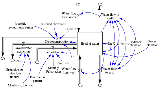
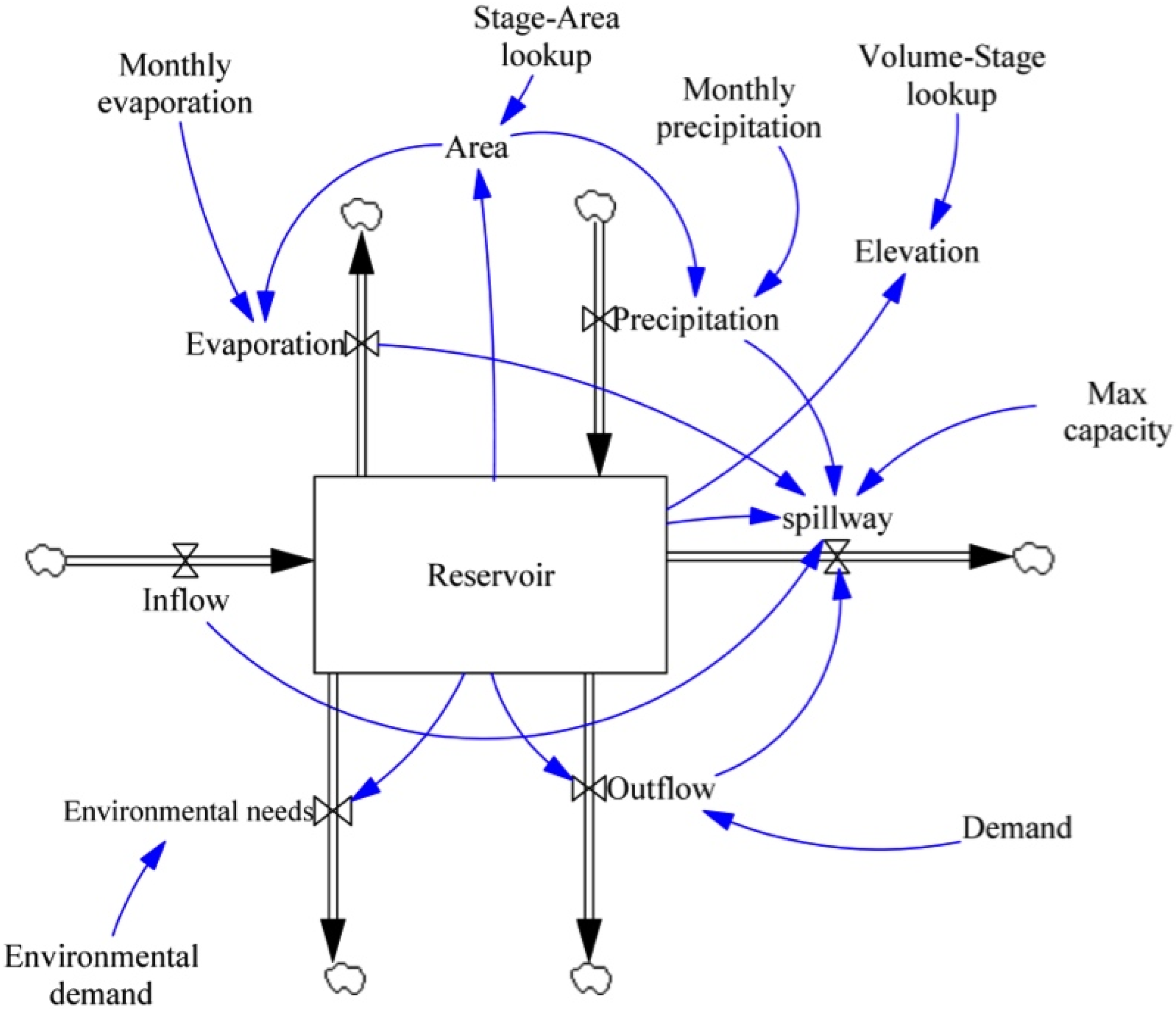
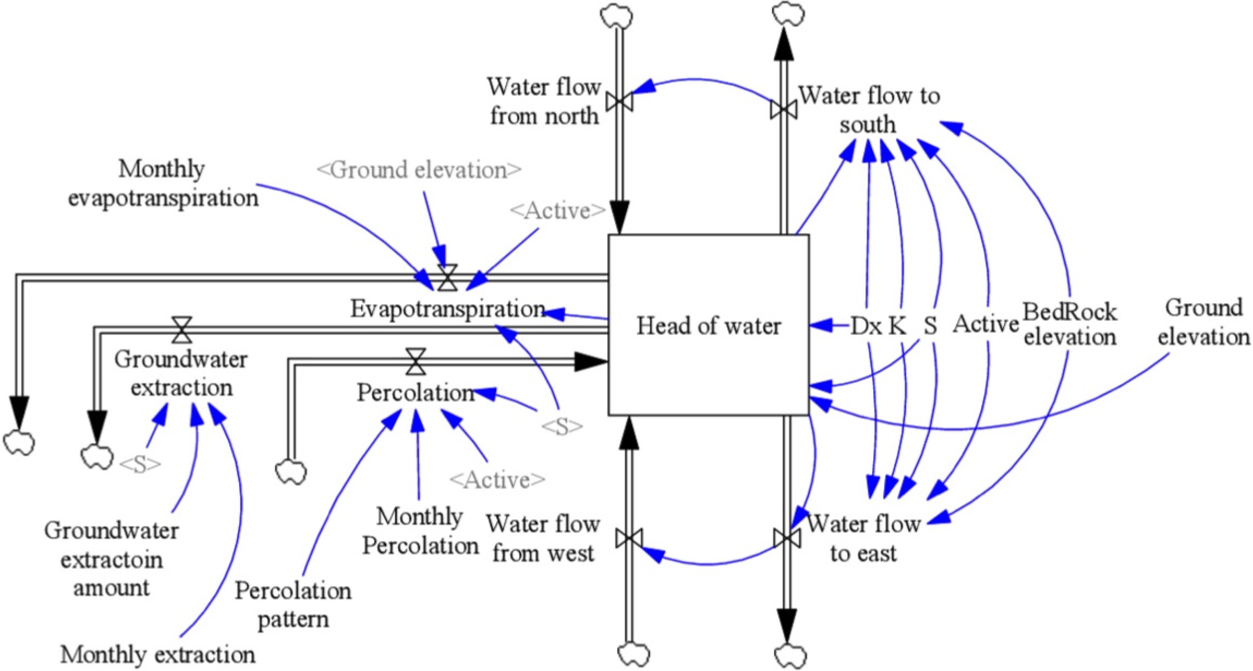
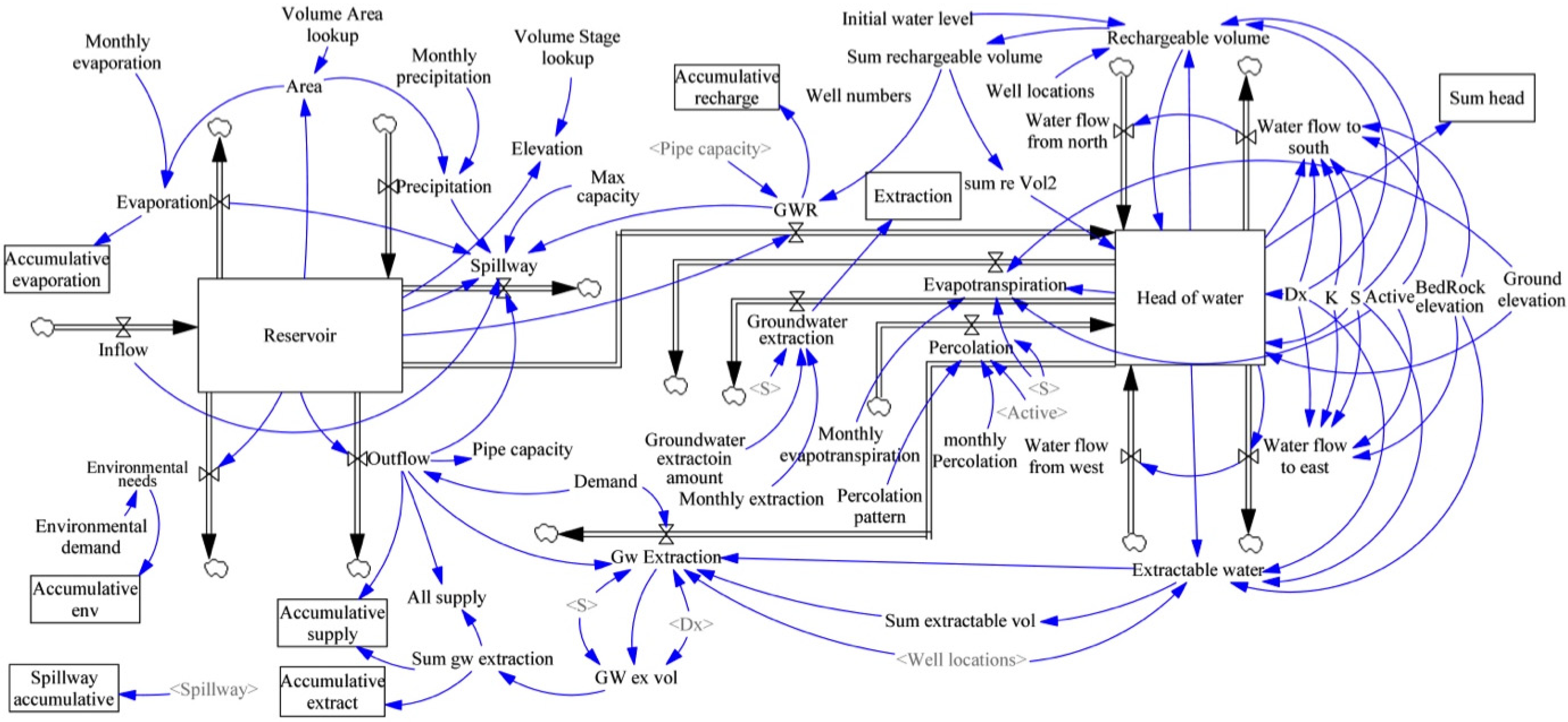
System Dynamics Model Conceptualization and Formulation

The system dynamics model in this study was developed using VENSIM [30] software. The model consists of two key segments, the reservoir model and the groundwater model. The ASR was modeled as a connection between these two segments. By taking into account the relevant components of the surface reservoir, the surface water reservoir segment of the model was the first to be built (Figure 1). This segment included a single level (reservoir), representing the volume of water in the reservoir at each time increment:
Reservoir = Inflow + Precipitation − Environmental needs − Outflow − Evaporation − Spillway discharge
Precipitation and inflow are the model’s two inputs. Precipitation represents the amount of water directly contributed to the reservoir by precipitation and is a function of the monthly precipitation rate and the expanse of water the reservoir represents. This rate was calculated by multiplying monthly precipitation by the reservoir’s surface area. Inflow is the river’s discharge into the reservoir. The inflow was calculated based on historical hydrological data for the river, imported through the “get Excel” data function in VENSIM.
Figure 1. System dynamics model of the surface water reservoir segment.
Water 06 02300 g001
Evaporation, Environmental needs, outflow and spillway discharge represent the model’s outputs. Evaporation, the volume of water evaporated from the reservoir surface at each time step, is a function of monthly evaporation and the reservoir’s surface area. This volume was calculated by multiplying monthly evaporation by the reservoir’s surface area. Monthly evaporation was derived from historical evaporation data for the study area and was introduced to the model by using the “get Excel” data function. At each time step, the reservoir surface area was taken from a volume-stage-area chart for the reservoir. Environmental needs and outflow were derived based on the allocated environmental needs and the irrigation water demand, respectively. Spillway discharge represents the excess water at each time step that exits the reservoir. Spillway discharge is a function of evaporation, precipitation, inflow, environmental needs, outflow, reservoir and the maximum (Max) capacity of the reservoir:
If (Inflow − Evaporation − Outflow + Precipitation + Reservoir) > Max capacity, then Spillway > 0)
If (Inflow − Evaporation − Outflow + Precipitation + Reservoir) < Max capacity, then Spillway = 0)
The groundwater modeling portion of the model was developed according to the spatial system dynamics (SSD) concept of a grid-based interaction of spatially-distributed system dynamics modules [28]. The SSD methodology has been used extensively in ecological modeling [31,32] and combines the powers of temporal and spatial analysis, achieved through systems dynamics and geographic information systems (GIS), respectively. This system was later used to model groundwater flow through compartmental spatial system dynamics (CSSD) [24]. Such a framework was intended to address issues related to groundwater and surface reservoir management.
The “stuck” head of water within the system dynamics model’s groundwater modeling segment is presented in Figure 2 and represents the head of water in each cell in the discretized aquifer domain. Each cell has flow toward four adjacent cells, located to its north, south, east or west. The head of water is a function of water flow from or toward the cell, water extraction from the cell, along with direct evapotranspiration and percolation. The water flow is calculated based on Darcy’s law. The head of water in the aquifer domain must be calculated based on the “subscript” function in VENSIM. The volume of water having entered or exited from the level is transformed into the head of water by dividing it by the area of the cell and the storage coefficient of the aquifer media. As square-shaped cells are used in this framework to simplify the modeling exercise, the cell area was the square of one side of the cell.
Figure 2. System dynamics model of the groundwater-modeling segment. Representing the active or inactive cells in the modeling domain, “active” is an auxiliary variable, which can also serve to define aquifer boundary conditions; S represents aquifer specific yield; Dx represents the length of one side of the cell; and K is the hydraulic conductivity of each cell in the aquifer.
Water 06 02300 g002
There were seven rates in this segment: water flow to south, water flow to east, water flow from the north, water flow from the west, percolation, evapotranspiration and groundwater extraction. Water flow toward or from adjacent cells were calculated in the first four rates of the last statement, and the three remaining rates account for the boundary flow from the top of the aquifer. Technically, water flow is calculated in two rates: water flow to the south and water flow to the east. Water flow from the west and water flow from the north are water flow to the east and water flow to the south of the previous cell. Based on Darcy’s law, water flow is a function of the media’s hydraulic conductivity, the head of the water in two adjacent cells and the length of the cell.
The occurrence of direct evapotranspiration from groundwater is a function of ground elevation, head of water and the region’s monthly evapotranspiration rate. If the head of water reaches within a certain distance of the ground surface, direct evapotranspiration can occur. This distance varies according to the aquifer media. Groundwater extraction and percolation are introduced to the model according to their monthly rates and pattern in the aquifer domain. In the groundwater modeling approach presented in this paper, the mass conservation concept was applied in each cell of the discretized aquifer (Figure 3).
Figure 3. Aquifer discretization and groundwater modeling paradigm in the system dynamics model.
Water 06 02300 g003
The change in storage in cell a is equal to the sum of the flow into a minus the sum of flow out of a to adjacent cells:
Water 06 02300 i005 = Qab + Qac + Qad + Qae + QaB
Where,
  • Water 06 02300 i006 is the change in storage through time in cell a (L3·T−1);
  • Qab,Qac,Qad,Qae is the flow into a from b, c, d and e, respectively, (L3·T−1); and
  • QaB is the sum of boundary flows to cell a (L3·T−1).
All flows are positive for flow into a and negative for flow out. Boundary flows are flow terms entering or leaving cell a, such as evaporation, evapotranspiration, natural recharge, artificial recharge and groundwater extraction. Ground water flow between two cells, Qab, can be described using Darcy’s law:
Water 06 02300 i007
where,
  • ha is the head of water in cell a (L);
  • hb is the head of water in cell b (L);
  • Ta is the transmissivity of cell a (L2·T−1);
  • Tb is the transmissivity of cell b (L2·T−1); and
  • x is the discrete distance used in the model (L).
By substituting Equation (4) and analogous terms for cells b, c and d, Equation (3) can be written as:
Water 06 02300 i008
Using a finite time step approximation for storage change, adding superscript notation to specify time and converting to matrix form for all possible generic ground water cells, Equation (4) can be rewritten to solve for storage in aquifer cell i at time t + 1 as a function of storage and head values at time t:
Water 06 02300 i009
where,
  • Water 06 02300 i010 is the flow in or out of cell i from four adjacent cells (L3·T−1);
  • Water 06 02300 i011 is the boundary flow (L3·T−1);
  • Water 06 02300 i012 is the storage of cell i at time t (L3·T−1);
  • Water 06 02300 i013 is the storage of cell i at time t + 1 (L3·T−1); and
  • t is the simulation time step (T).
This is a forward difference explicit solution for calculating groundwater heads in one time step from head values at the previous time step. Aquifer storage (Si) is related to aquifer head using the relationship between storage and head in an unconfined aquifer:
Si = (hi − Zbed) ∙ ∆x2 ∙ Sy
where,
  • Sy is the specific yield of the aquifer ;
  • Zbed is the bedrock elevation (L).
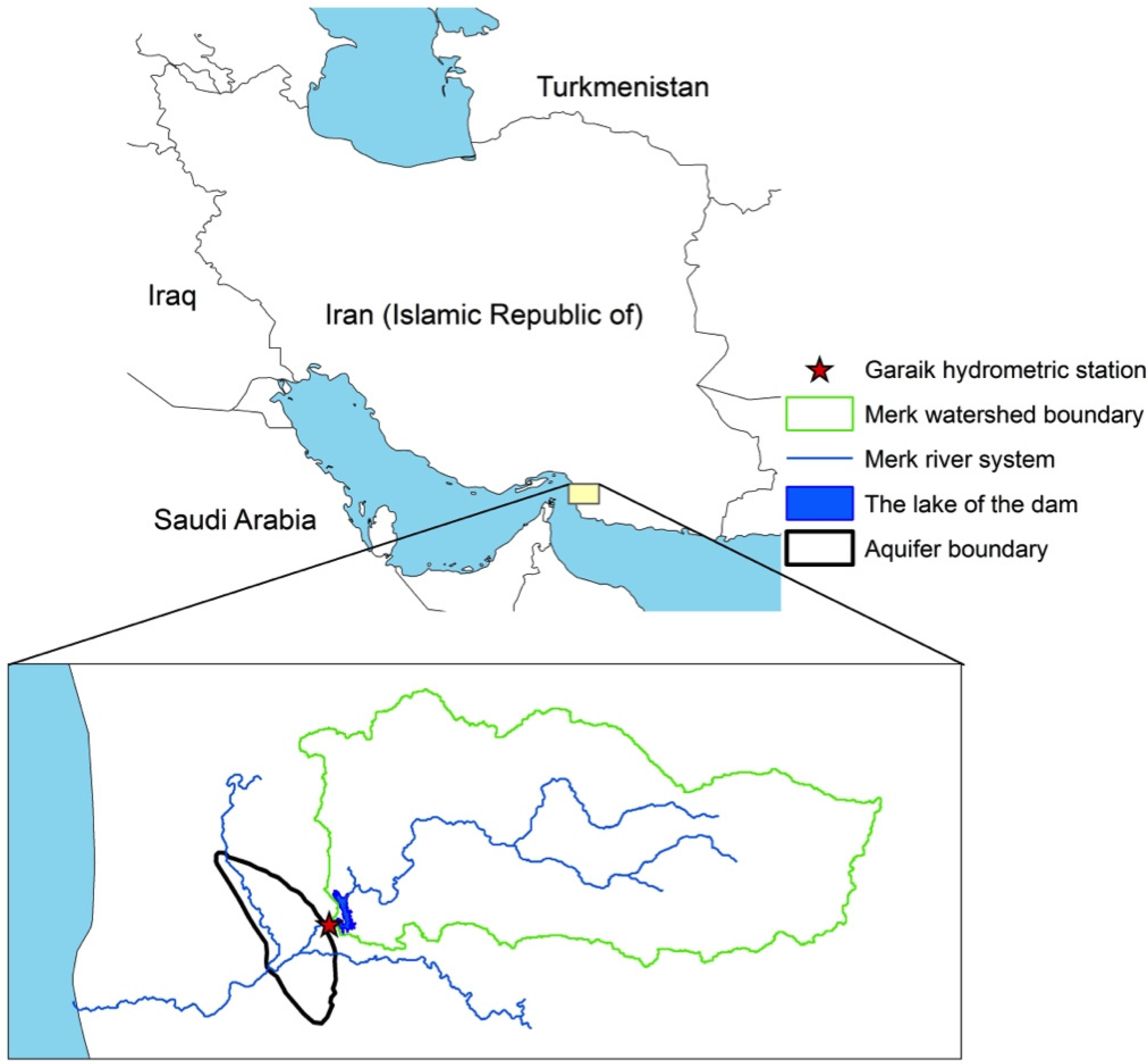
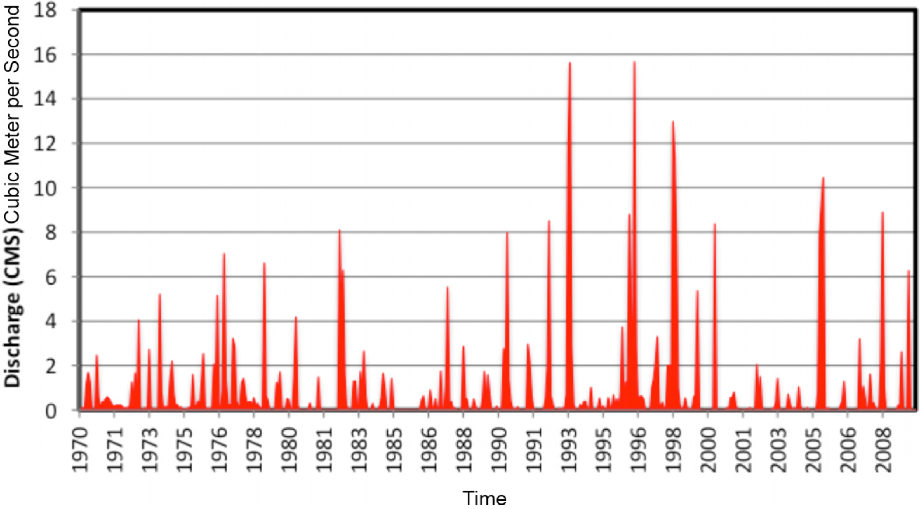
Because the forward difference explicit formulation calculates the future state based on the present state, the system of equations can be unstable if the time step is too long relative to the spatial scale and the rate of the movement of water between cells. Therefore, a small time step (such as 0.8 days, as was used in this study) must be used to prevent such a problem.
Having developed a surface water reservoir model and a groundwater model in the system dynamics environment, an ASR segment was added. This can be turned on/off automatically, as needed, in order to quantify the impacts of using ASR for the recharge or extraction of water from the aquifer. In the combined model, as illustrated in Figure 4, the left segment of the system represents the relevant components of the reservoir, while those on the right model groundwater in the aquifer based on the principles explained above.
The connection between the reservoir and the groundwater system is the groundwater recharge rate (GWR), fixed by the rate of water injection determined by the ASR approach. This rate is dependent on the availability of water in the reservoir, the pipeline capacity and the volume of rechargeable water in the groundwater system. As the purpose of the wells is to replenish depleted water, not to raise the water table above its original level, the rechargeable volume is based on the difference between the historical initial level and the actual level of the groundwater table in the cells containing ASR wells.
Figure 4. System dynamics model components.
Water 06 02300 g004

3. Study Area

3.1. Local Setting

The Sirik region, situated between 26°22' N and 26°43' N lat. and between 57°4' and 57°46' E long., houses an aquifer occupying 65 km2 on the southern edge of Hormuzgan Province, Iran. The Sirik region is semi-arid with mild winters (T = 22.3°C) and hot summers (T = 34.1°C). Average humidity ranges from 32.9% in the spring to a maximum of 71.9% in the winter. Mean annual temperature and precipitation are 28.2 °C and 190 mm, respectively, with the most rainfall occurring between October and December. The region has a population of approximately 11,667 people (2010), most of whom are engaged in agricultural production. The total amount of farmed land currently stands at ~1000 ha, with a mixture of vegetables, palm trees and citrus plantations. These crops were used in the modeling of the dam’s water resources and were selected based on their acceptance by farmers, as well as their production values. Agriculture is the main source of groundwater extraction, with total pumping amounting to 7.2 × 10⁶ m3·y−1. This pumping caused an average decline in groundwater levels of roughly 7 m between 2000 and 2010. It is also important to note that the region’s “river” is dry for most part of the year and only experiences flow during flash flood events. Flora and fauna, especially in the southern parts of the region, are more dependent on groundwater discharge than surface water availability. This strong dependency of plants on groundwater is mostly attributable to the fact that in the southern portion of the region, in the absence of surface water, groundwater is near the ground level and thereby available to plants.
The model developed in this study was for the Merk River watershed in the Sirik region; the dam, and the aquifer boundary locations are shown in Figure 5. This watershed drains 745 square kilometers, and the maximum elevation of the watershed is 1950 m above sea level (MASL), while the minimum elevation is 50 MASL. Daily discharge of the Merk River at the Garaik hydrometric station has been measured from 2006 to 2010. The location of the hydrometric station is also shown in Figure 5. Since the measurement’s time span was not sufficient for modeling the reservoir, the monthly time series of discharge was constructed for 40 years (1970–2010) by multivariate statistical analysis from nearby hydrometric stations. These analyses and data were derived from the feasibility study of the dam [33]. Subsequently, this monthly time series was used as the input flow to the reservoir model; the time series is shown in Figure 6.
Figure 5. Location of the dam’s watershed, watershed boundary, aquifer boundary and the Garaik hydrometric station.
Water 06 02300 g005
Figure 6. Time series of discharge at Garaik hydrometric station.
Water 06 02300 g006

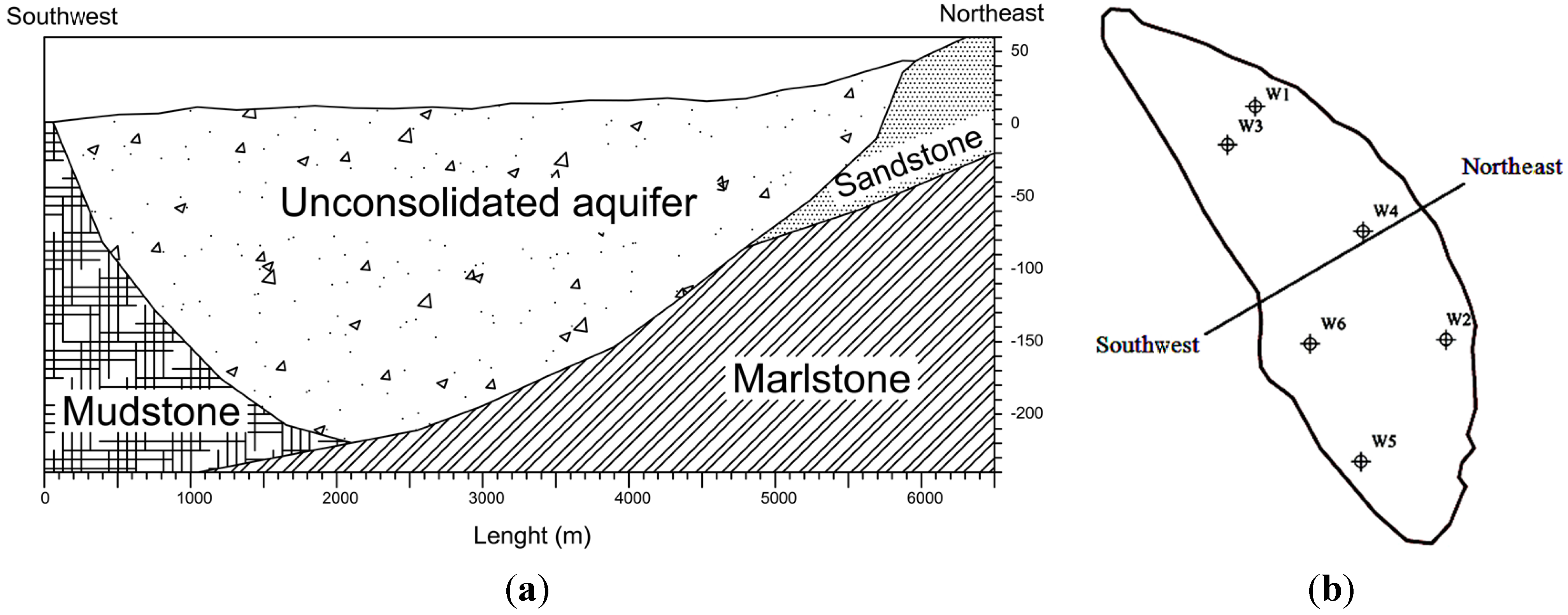
3.2. Hydrogeology of the Aquifer

The primary aquifer in this region is an unconfined and unconsolidated aquifer consisting of quaternary valley terrace deposits and river alluvial deposits (Figure 7a). The piezometric map of the region suggests that there is seepage from the northern sandstone to the aquifer. The bedrock is mostly middle Miocene marl with inter-bedded siltstone and sandstone. In the south, the aquifer is bounded by low permeable mudstone.
Figure 7. (a) Northeast to southwest cross-section of the Merk aquifer; (b) location of wells where pumping tests were conducted and the geological cross-section.
Water 06 02300 g007
Aquifer hydraulic properties were derived from six pumping tests using the AQTESOLV program with the Neuman method [34]. Figure 7b shows the location of these wells, while Table 2 provides their hydraulic properties and depths. This data was used in the modeling process and adjusted during the calibration process.
Table 2. Hydraulic conductivity and specific storage of different regions of the aquifer.
Well nameWell depth (m)Hydraulic conductivity (m2·s−1)Specific yield
W1508.4 × 10−50.05
W2408.7 × 10−50.06
W3701.1 × 10−60.08
W4701.3 × 10−60.011
W5605.6 × 10−60.011
W6904.7 × 10−60.014
Based on the different soil types and land uses, three recharge zones were assigned in the plain (Figure 8a). Most recharge is due to seepage from sandstone to the aquifer, with some recharge from riverbeds and precipitation. The preliminary estimation of recharge was based on an estimation of water balance components and then adjusted during the model calibration.
Since 2000, 10 observation wells have been installed and water elevation recorded on a monthly basis. This data served in calibrating and validating the groundwater model.
Figure 8. (a) Different recharge zones in the aquifer; (b) elevation-area-volume graph of Merk dam reservoir before and after sedimentation.
Water 06 02300 g008

3.3. Dam/Reservoir Characteristics

As proposed and if constructed, the Merk dam would be an earth-filled dam with a clay core. The normal elevation would be 91 m above mean sea level (AMSL), and the capacity of the reservoir after maximum sedimentation would be 40 × 106 m3. The source of water to fill the reservoir would be the Merk River. The river’s mean annual stream flow is 25.9 × 10⁶ m3. An elevation-area-volume chart of this dam (Figure 8b) was used to estimate the rate of evaporation from the reservoir in the system dynamics model developed in our study. This information was derived from a feasibility study report on the Merk dam approved by the Iranian Ministry of Energy [33]. The water supplied from the dam would be conveyed through a pipeline to agricultural areas. According to dam design reports, the mean irrigation demand of the dam’s command areas would be 8013 m3·ha−1·y−1, oscillating between 2860 and 12,710 m3·ha−1·y−1. Figure 9a presents a schematic view of the dam, aquifer and agricultural lands [33].
Figure 9. (a) Schematic view of the proposed system, consisting of the dam, agricultural areas within the aquifer boundaries and a pipeline to convey water from the dam to agricultural areas; (b) discretization of the aquifer system and its side views.
Water 06 02300 g009
Under Iranian governmental regulations [33], a certain percentage of a river’s average natural flow must be allowed to remain flowing throughout the river course. This percentage is 10% during the wet seasons and 30% during the dry seasons. Consequently, this amount of water was considered the minimum environmental requirement of the river in the model.

4. Methodology

A conceptual model of the region’s groundwater flow was initially developed, then translated to computational form through the use of MODFLOW [35] software. The conceptual model was developed based on information presented in the section “Hydrogeology of the Aquifer”. The aquifer was discretized to 45 × 35 cells, with each cell representing an area of 350 m × 350 m (Figure 9b).
The model was calibrated and run using hydrogeological data and aquifer characteristics (Table 2) collected from 2000 to 2005 by regional hydrological experts. The model was then validated using similarly obtained data for the period of 2006 to 2010 using the RMSE performance index. Once the groundwater flow had been modeled using MODFLOW, the information gained was used to build a system dynamics model of the aquifer (Figure 2).
The system dynamics groundwater model was subsequently evaluated against the MODFLOW results. In the next stage, four different ASR implementation scenarios were developed and tested using the comprehensive system dynamics model. The system dynamics model as mentioned formerly has the ability to model concurrently the dam, groundwater system and ASR. Lastly, an economic analysis was undertaken to evaluate each of the different scenarios.

4.1. Scenarios

To assess the best approach to optimize the expanse of land to be converted to new farmland while maintaining appropriate environmental flows from the dam, as well as manageable spillway flows, along with a sustainable groundwater balance, four scenarios were evaluated using the system dynamics model. In all scenarios, the government’s goal of adding 1000 ha of new agricultural land was respected. These lands will be referred to as “additional command areas” from now on. In order to gauge its potential economic impact, two different dam heights, resulting in initial reservoir volumes of 20 × 106 m3 or 40 × 106 m3, were compared in Scenarios 220, 240, 320, 340, 420 and 440, respectively. In the baseline scenario, 1, only the taller dam/larger reservoir option was modeled, and this scenario was represented as 140.
Scenario 1: baseline scenario, in which the dam’s effects on the water table are modeled as the dam’s implementation is currently proposed (without any inclusion of an ASR approach). Water trapped in the reservoir flows to farmers’ fields (old and new) through a constructed irrigation network.
Scenario 2: 40 new injection wells are constructed throughout the region, from which reservoir water is pumped under high pressure into the aquifer. Farmers continue to make use of their existing boreholes for extraction, while also using the injection wells as pumps during recovery periods.
Scenario 3: 40 new high-pressure injection wells are constructed while existing boreholes are shut down, forcing farmers to rely upon the stored water from the new sites. In this scenario, the existing agricultural lands, which were irrigated by farmers’ wells, will be rehabilitated. The rehabilitation of the existing lands will add some costs into the project, but on the other hand, will increase the irrigation efficiency and productivity of the farms that will result in more benefit for the project.
Scenario 4: no new high-pressure injection wells are constructed; rather, water from the reservoir flows via gravity into existing borehole wells spread-out across the current 1000 ha of agricultural land. All additional new land is watered directly from the reservoir through a constructed irrigation network.

4.2. Economic Analysis

For economic analysis, a cost/benefit of investment approach was applied, where the net present value of an investment was calculated by using a discount rate and a series of future payments (negative values) and incomes (positive values). Incomes were based on net economic gains of agricultural activities, valued at 3,556 USD ha−1·y−1, based on average prices of cultivated crops in the region [33]. The cost components of the economic analysis are listed in Table 3.
Table 3. Potential costs involved in the aquifer storage and recovery (ASR) project in Sirik, Iran.
Economic ComponentsValueUnit
Irrigation network6,500USD ha−1
Installation of each injection well50,000USD per well
Building dam with 40 × 106 m3 reservoir22,239,000USD
Building dam with 20 × 106 m3 reservoir9,850,000USD
Modifying an existing well15,000USD
Dam lifetime50Years
Cost of operation and maintenance of dam2% of building cost per year
Cost of operation and maintenance of irrigation network5% of building cost per year
Construction duration2Years
Education of farmers towards using ASR in scenario 4200,000USD
Interest rate7Percent
Engineering services8% of construction cost
Averaged agricultural gains3,556USD ha−1

5. Results

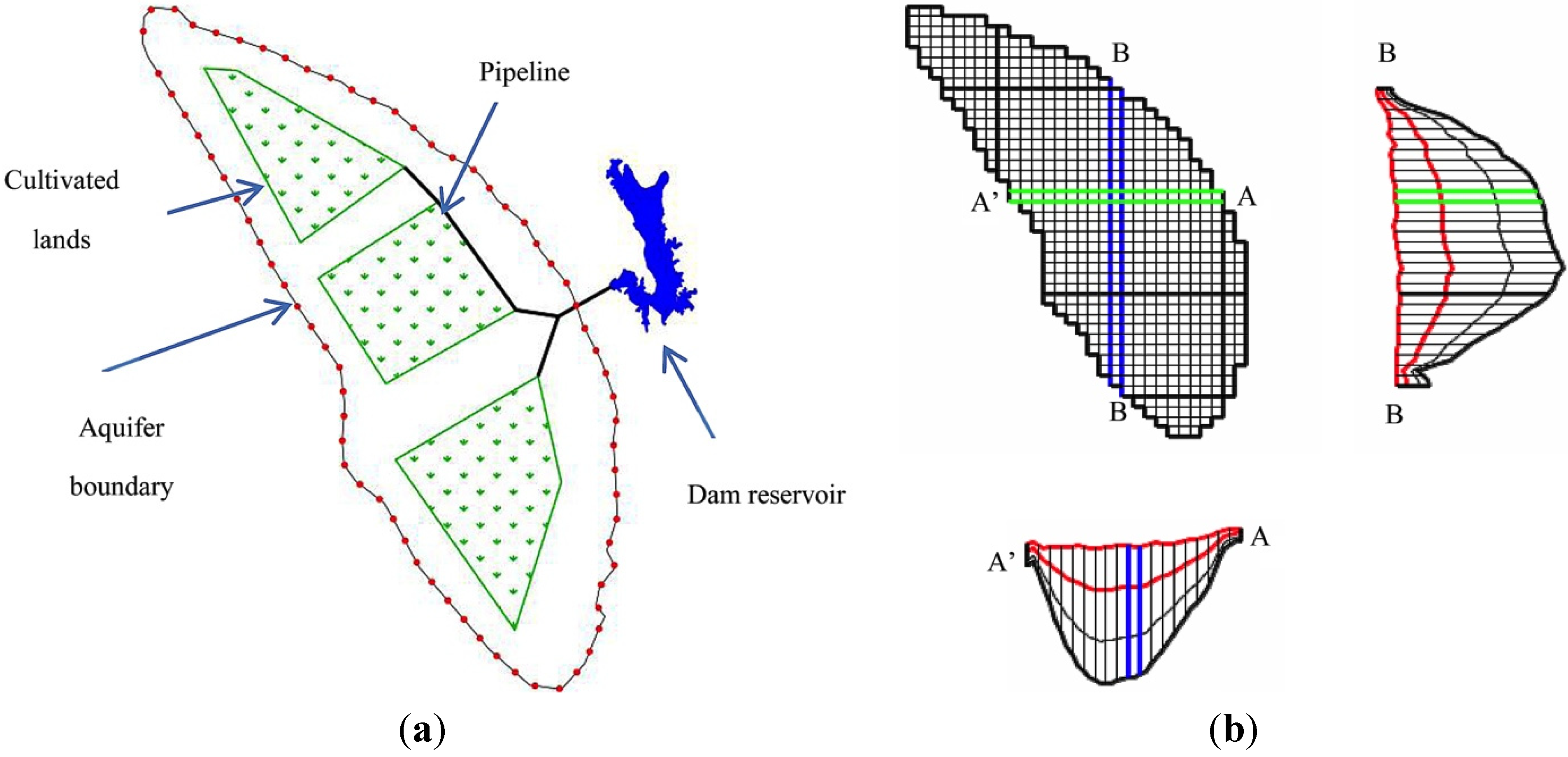
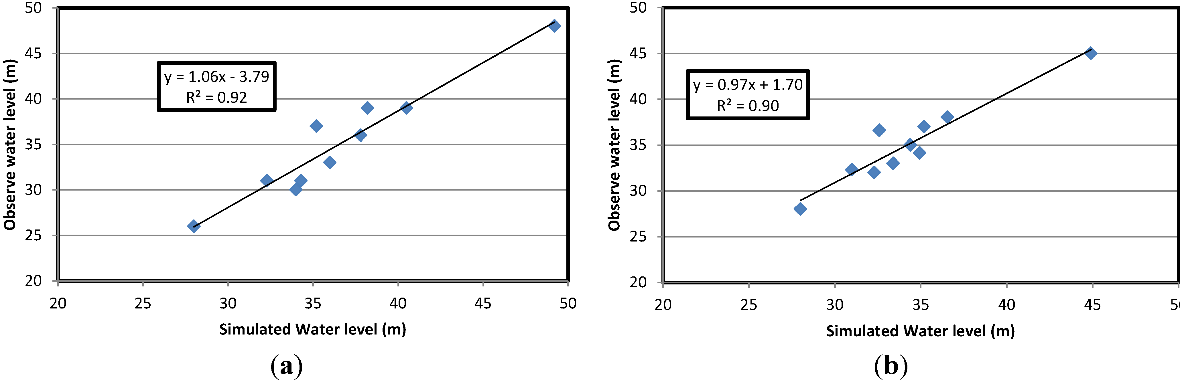
5.1. Results of Aquifer Model Implemented with MODFLOW

Modelmate software and UCODE were used to calibrate MODFLOW. Recharge, hydraulic conductivity and specific yield were introduced as parameters to Modelmate. The model results were then compared with the head measurement in 10 observation wells across the aquifer. The calibration coefficient was 0.92 in the calibration stage (Figure 10a). For validation, correlation coefficients (R2) reached 0.90. The root mean square error (RMSE) at the end of calibration and evaluation of the model was around one meter (Figure 11b). The results show that the conceptual groundwater model is capable of capturing the major processes in the groundwater system in the aquifer.
Figure 10. (a) Simulated water table vs. observed water table for the calibration period. (b) Simulated water table vs. observed water table for the validation period.
Water 06 02300 g010

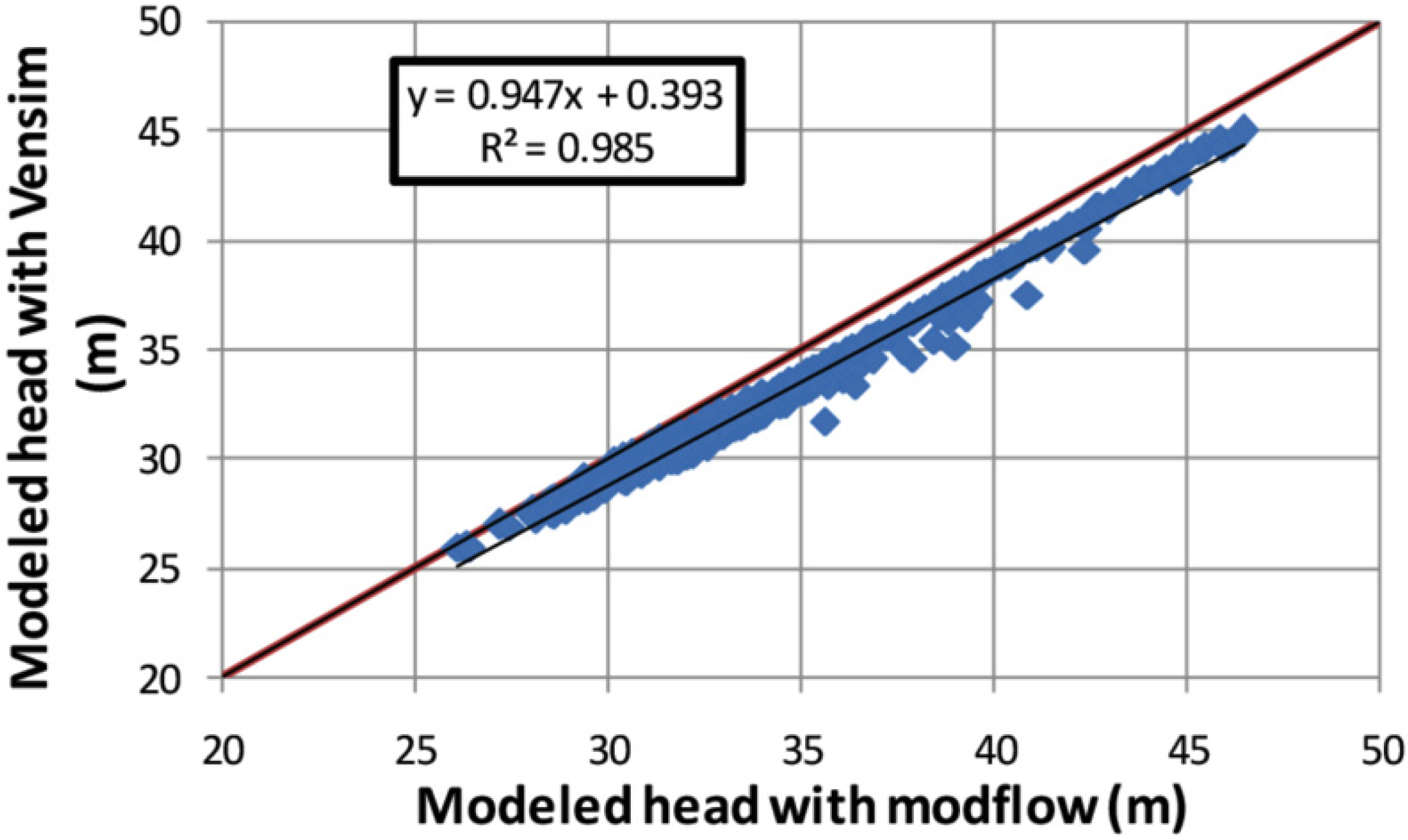
5.2. Comparison of VENSIM/MODFLOW Results

In this stage, all calibrated data were transferred to the VENSIM software, and this model was run without considering the effect of the dam and ASR system on the aquifer for a period of 10 years to examine whether the groundwater model component of the system dynamics model had the ability to model the groundwater system effectively. Results showed an R2 = 0.95 between the MODFLOW and VENSIM models and an RMSE < 1 m (Figure 11). In Figure 12, the results of the simulation of Scenario 1 and 4 at maximum reservoir capacity are presented.
Figure 11. Correlation between MODFLOW results and VENSIM results.
Water 06 02300 g011
Figure 12. Models results for Scenarios 1 and 4: (a) accumulative evaporation; (b) average water table of the aquifer: and (c) water storage in the reservoir.
Water 06 02300 g012

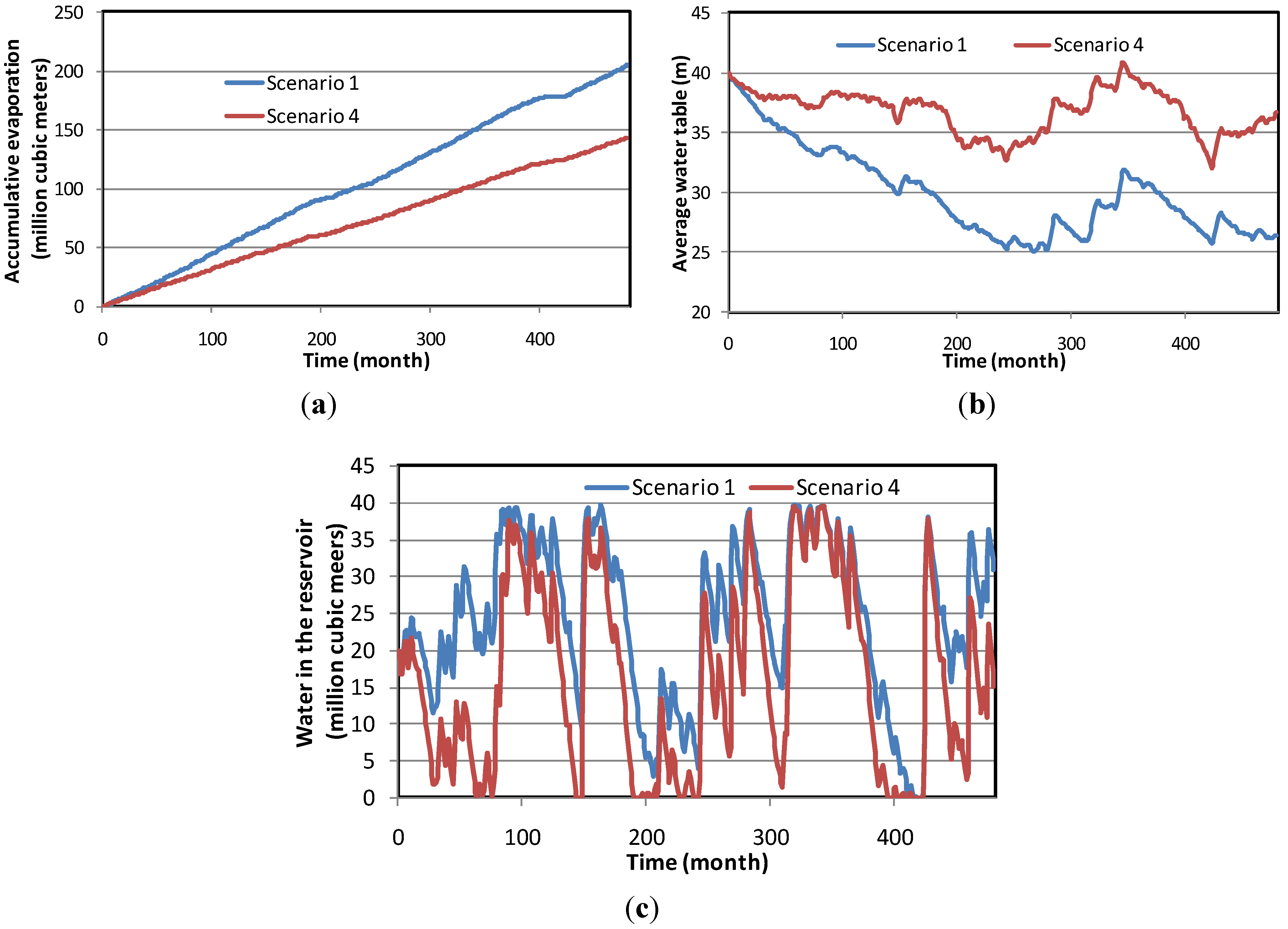
5.3. System Dynamics and Economic Analysis Results

The results of the modeling with system dynamics and economic analysis are shown in Table 4. All scenarios had the same amount of inflow, as this was generated by the floodwaters captured by the reservoir (Table 4). Water lost to evaporation (106 m3) varied greatly amongst the scenarios, with 205.1 lost under the “business as usual” scenario (140), 100.1 and 156.9 under Scenarios 220 and 240, 71.7 and 118.2 under Scenarios 320 and 340 and 98.6 and 153.5 under Scenarios 420 and 440. Environmental flow (106 m3) from the dam varied, from 153.4 under Scenario 140, to 130.7 and 144.5 under Scenarios 220 and 240, 117.0 and 130.3 under Scenarios 320 and 340 and 129.9 and 143.6 under Scenarios 420 and 430. Spillway flow from the dam (106 m3) also varied, from a high of 423.6 under Scenario 140, to 342.0 and 227.3 under Scenarios 220 and 240, 290.9 and 186.0 under Scenarios 320 and 340 and 340.5 and 222.7 under Scenarios 420 and 440.
The average drawdown of the water table varied from a high of 14.5 m under Scenario 140, to 5.4 m and 3.2 m under Scenarios 220 and 240, 2.4 m and 0.9 m under Scenarios 320 and 340 and 5.3 m and 3.0 m under Scenarios 420 and 440. The total costs of implementation varied, from a low of $37,296,000 under Scenario 140 (the basic cost of the dam and irrigation network), to $41,258,000 and $40,112,000 under Scenarios 220 and 240 (the costs of the dam, irrigation network, 40 new injection wells, as well as the price of pumped water), $55,983,000 and $51,082,000 for Scenarios 320 and 340 (the cost of the dam, irrigation network, 40 new injection wells, as well as the price of pumped water) and, finally, $41,597,000 and $37,407,000 for Scenarios 420 and 440 (the cost of the dam, irrigation network and modifications to existing boreholes).
Table 4. Water supply and economic analysis of scenarios after 40 years of simulation. Note that for Scenarios 2, 3 and 4, each scenario compared two dam heights resulting in initial reservoir volumes of 20 × 106 m3 or 40 × 106 m3.
Scenario 1Scenario 2Scenario 3Scenario 4
Initial reservoir volume (106 m3)40204020402040
Inflow (106 m3)1,036.51,036.51,036.51,036.51,036.51,036.51,036.5
Environmental flow (106 m3)153.4130.7144.5117.0130.3129.9143.6
Agriculture (106 m3)313.4251.7284.9373.4464.1249.9282.7
Command area (additional) (ha)1,000.01,000.01,000.01,000.01,000.01,000.01,000.0
Improved command area (ha)0.00.00.01,000.01,000.00.00.0
Existing area (no change) (ha)1,000.01,000.01,000.00.00.01,000.01,000.0
Evaporation (106 m3)205.1100.1156.971.7118.298.6153.5
Spillway (106 m3)423.6342.0227.3290.9186.0340.5222.7
Unregulated water (106 m3)577.0472.7371.8407.8316.2470.4366.2
Pumping (106 m3)0.067.934.6265.77175.169.736.9
Injection (106 m3)0.0215.6227.7227.7151.7221.2238.9
Average water table’s elevationStart (m)39.939.939.939.939.939.939.9
End (m)25.434.636.837.639.134.637.0
Average drawdown (m)14.55.43.22.40.95.33.0
Normal elevation of dam (m)91859185918591
Benefit (USD)49,075,00049,075,00049,075,00056,436,00056,437,00049,075,00049,075,000
Cost (USD)37,296,00041,258,00040,112,00055,983,00051,083,00041,597,00037,407,000
B/C1.321.191.221.011.101.181.31
B-C (USD)11,779,0007,817,0008,964,000454,0005,354,0007,478,00011,669,000

6. Discussion

6.1. Consequences of “Business as Usual”

From a water management perspective, the proposed standard reservoir and dam system planned for the Sirik region is poorly thought out, given the significant quantity of water lost to evaporation (about 25% more than any other scenario). Furthermore, continued extraction of groundwater with no plan to replenish the aquifer would lead to a water table level drawdown of 14.5 m over the next 40 years, a case that would not only greatly increase the difficulty and cost of pumping water for agriculture and endangering people’s livelihoods, but also threaten local wildlife that depend on shallow groundwater levels in the southwest portion of the Sirik region. It is thus suggested that a new paradigm of groundwater management be adopted in the region that makes use of ASR to prevent losses through evaporation and slows the rate of groundwater drawdown.

6.2. Scenario Selection Based on Cost/Benefit Analysis

To decide the most appropriate scenario for the development of Sirik, we rely on a variety of criteria to determine which scenario provides the best return on investment. The first is the cost/benefit analysis, which takes into account the total costs (C) of a scenario, weighed against the expected financial benefits (B) from expanded agricultural production in the region. The two scenarios that provide the greatest return on investment are Scenario 140 and Scenario 440; however, return on investment is not the only criterion for acceptability. Scenario 340 provides the greatest reduction in drawdown over 40 years, at 0.9 m, compared to 3.0 m for Scenario 440 or 3.2 m for Scenario 240. However, scenario 340’s slower rate of drawdown comes at an additional cost of $13,650,000, while only allowing 84.5% of the originally planned environmental flow. Lastly, the need for farmers to shut down their own wells and to rely solely on newly installed high-pressure injection wells poses problems of social acceptability.
Though Scenario 440 has higher rates of evaporation than Scenario 340 and a similar rate of evaporation as Scenario 240, it remains the most cost-effective scenario, providing for a manageable quantity of spillway flow (that when unmanaged can lead to flooding damage), as well as the highest proportion of the original environmental flow (93.57%). As the southern ecosystem that sustains the region’s native flora and fauna depends on a shallow groundwater table, it is justifiable to transfer some water from environmental flow into the aquifer in order to maintain upwelling and springs.
Scenario 3 has more benefits and costs than the other scenarios. As it was formerly explained, in this scenario, the irrigation system in existing farmlands should be rehabilitated, so that there would be a cost associated with the rehabilitation that will be added to the base cost of the project. On the other hand, the modified system will elevate crop production, and as a result, benefits would also increase. However, the cost of the project in this scenario outweighs the benefit; thus, the benefit over the cost of this scenario is less than for the other scenarios.

6.3. Social Acceptability and Sustainability

Scenario 440 is the most socially acceptable and sustainable of the solutions, allowing farmers to keep their own wells on their land and for them to be improved at no cost to the farmer. Unlike Scenarios 240 and 340, Scenario 440 does not require the installation of complex high-pressure injection and pumping stations, which require technical upkeep and repairs, but instead makes use of improved boreholes on existing plots. Technical and managerial training programs for farmers would be promoted, in order to provide users with the skills to maintain their own systems and manage water use. Through choosing to work through existing social networks and demonstrating willingness to engage, the project could gain local support from the farmers. This type of public engagement and empowerment is a central tenet of the new paradigm of integrated water resources management and sets the groundwork for farmer-led groundwater management.

6.4. Uncertainty Due to Climate Variability and Climate Change

Although the models benefited from 40 years of historical hydro-climatological time series data, climate variability and climate change results in uncertainties concerning the modeling results of all scenarios. Regarding climate variability, different combinations of wet and dry hydro-climatological input parameters of the model (inflow, recharge, evaporation, etc.) will affect the results of each scenario. Nevertheless, since the model input parameters are the same in all scenarios, the variation between scenarios will remain relatively similar to the current study, so the deviation would not be substantial. On the other hand, climate change could have a major impact on the results, since it is believed that the input parameters of the model will no longer remain stationary in the future. It is predicted that climate change will cause more severe extreme events (floods and droughts) in this region [36]. In this situation, conjunctive use should be more beneficial than conventional water management schemes. Conjunctive use (Scenarios 2, 3 and 4) under severe drought conditions is more advantageous than merely relying on surface water.
This study introduced a new modeling tool, which also opens a new avenue to assess uncertainties due to climate variability and climate change in future studies. In order to address uncertainty in future studies, different sets of climate variables (precipitation and temperature) should be derived from downscaled climate change models, and then, this climate data can be used in hydrologic models to estimate discharge in the watershed. The output from the hydrological model can subsequently be used as an input to the SD model to build a set of results. The probability distribution function can then be derived from the results of the SD model to assess the uncertainty associated with climate change.

7. Conclusions

The objective of this study was to examine if ASR, in conjunction with water storage on an ephemeral river, could be an effective water resource management strategy that would minimize both water lost to evaporation and the rate of groundwater depletion, while providing water for expanded agricultural activities. It was determined that this approach can significantly improve the sustainability of groundwater supplies. It must be emphasized that the future development of the Sirik region must include a water management approach of groundwater storage and recovery. In so doing, significant gains can be achieved at a minimal cost. By modeling groundwater flow and whole system dynamics, ASR was shown to be an applicable and beneficial strategy for the well-being of farmers and the region’s groundwater system. Without the inclusion of ASR, the region will face grave consequences due to unsustainable exploitation of groundwater. However, through a combination of central technical planning, ASR strategies and farmer engagement and education, the current proposal has the potential to help direct the future development of the region in a sustainable manner.
The system dynamics modeling framework developed and implemented in this study was shown to be very effective. Not only groundwater, but a surface water reservoir was modeled in a single program. This modeling approach can be expanded and used in different areas where a combination of groundwater and surface water are considered as sources of a water supply system. Interconnection technologies, such as ASR, can also be addressed in this modeling approach, something not easily accomplished in other modeling frameworks. Although the groundwater modeling portion of the model was developed for an unconfined aquifer, it is relatively simple, using the same mathematical concepts, to develop such a model for a confined aquifer.
Another advantage of such a modeling approach is that groundwater and surface water reservoirs are completely linked to each other and in each time step; each model is updated with the output of the other model. This mutual relationship enables one to solve the problem with greater accuracy and fewer simplifying assumptions.

Acknowledgements

The authors would like to thank David Dean, Nicole Guo and Naeem Ahmed for their assistance in the preliminary stages of this research. The authors would also like to take this opportunity to thank two anonymous editors who improved the quality of this research with their very useful comments.

Author Contributions

Amir Niazi conceived the idea of this research, conducted the SD modeling, economical analysis and writing of the manuscript. Shiv Prasher funded the research and provided recommendations, which improved the system dynamics model. Jan Adamowski provided feedback regarding the SD models and modified the manuscript throughout the project. Tom Gleeson helped conceptualize the groundwater system in the study area, as well as the groundwater modeling in the SD models.

Conflicts of Interest

The authors declare no conflict of interest.

References

  1. Giordano, M.; Villholth, K.G. The Agricultural Groundwater Revolution: Opportunities and Threats to Development; CABI (Commonwealth Agricultural Bureaux International): London, UK, 2007; p. 419. [Google Scholar]
  2. Gleeson, T.; VanderSteen, J.; Sophocleous, M.A.; Taniguchi, M.; Alley, W.M.; Allen, D.M.; Zhou, Y.X. Groundwater sustainability strategies. Nat. Geosci. 2010, 3, 378–379. [Google Scholar] [CrossRef]
  3. Theis, C.V. The source of water derived from wells essential factors controlling the response of an aquifer to development. Civil Eng. 1940, 10, 277–280. [Google Scholar]
  4. Freeze, R.A.; Cherry, J.A. Groundwater; Prentice Hall Inc. Publishers: Upper Saddle River, NJ, USA, 1979; p. 604. [Google Scholar]
  5. Khana, S.; Mushtaqb, S.; Hanjraa, M.A.; Schaefferd, J. Estimating potential costs and gains from an aquifer storage and recovery program in australia. Agric. Water Manag. 2008, 95, 477–488. [Google Scholar] [CrossRef]
  6. Bouwer, H. Artificial recharge of groundwater: Hydrogeology and engineering. Hydrogeol. J. 2002, 10, 121–142. [Google Scholar] [CrossRef]
  7. Bouwer, H. Integrated water management: Emerging issues and challenges. Agric. Water Manag. 2000, 45, 217–228. [Google Scholar] [CrossRef]
  8. Sedighi, A. A Quasi-Analytical Model to Predict Water Quality during the Operation of an Aquifer Storage and Recovery System; University of Florida: Gainesville, FL, USA, 2003. [Google Scholar]
  9. Topper, R.; Barkmann, P.E.; Bird, D.A.; Sares, M.A. Artificial Recharge of Groundwater in Colorado; Colorado Geological Survey: Denver, CO, USA, 2004. [Google Scholar]
  10. Maliva, R.; Missimer, T. Arid Lands Water Evaluation and Management; Springer: Berlin/Heidelberg, Germany, 2012; Volume 1, p. 1076. [Google Scholar]
  11. Dillon, P. Future management of aquifer recharge. Hydrogeol. J. 2005, 13, 313–316. [Google Scholar] [CrossRef]
  12. Kalantari, N.; Rangzan, K.; Thigale, S.S.; Rahimi, M.H. Site selection and cost-benefit analysis for artificial recharge in the baghmalek plain, khuzestan province, southwest iran. Hydrogeol. J. 2010, 18, 761–773. [Google Scholar] [CrossRef]
  13. Todd, D.K.; Mays, L.W. Groundwater Hydrology, 3rd ed.; Wiley: Hoboken, USA, 2005. [Google Scholar]
  14. Pulido-Velazquez, M.; Jenkins, M.W.; Lund, J.R. Economic values for conjunctive use and water banking in southern california. Water Resour. Res. 2004, 40. [Google Scholar] [CrossRef]
  15. Kern Water Bank Authority. Available online: http://www.kwb.org/index.cfm/fuseaction/Pages.Page/id/330 (accessed on 20 March 2014).
  16. Sahuquillo, A.S. Conjunctive Use of Surface Water and Groundwater; Encyclopedia of Life Support Systems (EOLSS): Paris, France, 2004; Volume III. [Google Scholar]
  17. Stave, K. Participatory system dynamics modeling for sustainable environmental management: Observations from four cases. Sustainability 2010, 2, 2762–2784. [Google Scholar] [CrossRef]
  18. Geurts, J.L.A.; Joldersma, C. Methodology for participatory policy analysis. Eur. J. Oper Res. 2001, 128, 300–310. [Google Scholar] [CrossRef]
  19. Stave, K.A. Using system dynamics to improve public participation in environmental decisions. Syst. Dyn. Rev. 2002, 18, 139–167. [Google Scholar] [CrossRef]
  20. Winz, I.; Brierley, G.; Trowsdale, S. The use of system dynamics simulation in water resources management. Water Resour. Manag. 2009, 23, 1301–1323. [Google Scholar] [CrossRef]
  21. Giordano, R.; Brugnach, M.; Vurro1, M. System dynamic modelling for conflicts analysis in groundwater management. In International Congress on Environmental Modelling and Software, Managing Resources of a Limited Plane; Seppelt, R., Voinov, A.A., Lange, S., Bankamp, D., Eds.; International Environmental Modelling and Software Society (iEMSs): Leipzig, Germany, 2012; p. 10. [Google Scholar]
  22. Abbott, M.D.; Stanley, R.S. Modeling groundwater recharge and flow in an upland fractured bedrock aquifer. Syst. Dyn. Rev. 1999, 15, 163–184. [Google Scholar] [CrossRef]
  23. Leaver, J.D.; Unsworth, C.P. System dynamics modelling of spring behaviour in the orakeikorako geothermal field, New Zealand. Geothermics 2007, 36, 101–114. [Google Scholar] [CrossRef]
  24. Roach, J.; Tidwell, V. A compartmental-spatial system dynamics approach to ground water modeling. Ground Water 2009, 47, 686–698. [Google Scholar] [CrossRef]
  25. Langsdale, S.; Beall, A.; Carmichael, J.; Cohen, S.; Forster, C. An exploration of water resources futures under climate change using system dynamics modeling. Integr. Assess. J. 2007, 7, 51–79. [Google Scholar]
  26. Xu, Z.X.; Takeuchi, K.; Ishidaira, H.; Zhang, X.W. Sustainability analysis for yellow river water resources using the system dynamics approach. Water Resour. Manag. 2002, 16, 239–261. [Google Scholar] [CrossRef]
  27. Karavezyris, V.; Timpe, K.P.; Marzi, R. Application of system dynamics and fuzzy logic to forecasting of municipal solid waste. Math. Comput. Simul. 2002, 60, 149–158. [Google Scholar] [CrossRef]
  28. Ahmad, S.; Simonovic, S.P. Spatial system dynamics: New approach for simulation of water resources systems. J. Comput. Civil Eng. 2004, 18, 331–340. [Google Scholar] [CrossRef]
  29. Wang, X.-J.; Zhang, J.-Y.; Liu, J.-F.; Wang, G.-Q.; He, R.-M.; Elmahdi, A.; Elsawah, S. Water resources planning and management based on system dynamics: A case study of yulin city. Environ. Dev. Sustain. 2011, 13, 331–351. [Google Scholar] [CrossRef]
  30. Eberlein, R.L.; Peterson, D.W. Understanding models with vensim™. Eur. J. Oper Res. 1992, 59, 216–219. [Google Scholar] [CrossRef]
  31. Deal, B.; Farello, C.; Lancaster, M.; Kompare, T.; Hannon, B. A dynamic model of the spatial spread of an infectious disease: The case of fox rabies in illinois. Environ. Model. Assess. 2000, 5, 47–62. [Google Scholar] [CrossRef]
  32. Costanza, R.; Voinov, A.; Boumans, R.; Maxwell, T.; Villa, F.; Wainger, L.; Voinov, H. Integrated ecological economic modeling of the patuxent river watershed, maryland. Ecol. Monogr. 2002, 72, 203–231. [Google Scholar] [CrossRef]
  33. Morshedian, H. Feasibility Study of Merk Dam; Regional Water Co. Ministry of Energy: Tehran, Iran, 2012; p. 871. [Google Scholar]
  34. Neuman, S.P. Effect of partial penetration on flow in unconfined aquifers considering delayed gravity response. Water Resour. Res. 1974, 10, 303–312. [Google Scholar] [CrossRef]
  35. Harbaugh, A.W. MODFLOW-2005, the U.S. Geological Survey Modular Ground-Water Model—The Ground-Water Flow Process: U.S. Geological Survey Techniques and Methods 6-a16; USGS: Reston, VA, USA, 2005. [Google Scholar]
  36. Amiri, M.J.; Eslamian, S.S. Investigation of climate change in Iran. J. Environ. Sci. Technol. 2010, 3, 208–216. [Google Scholar] [CrossRef]

