Impact of Forest Cover and Aridity on the Interplay between Effective Rooting Depth and Annual Runoff in South-West Western Australia

Abstract

Variants of the Budkyo hydrological model describe the effects of land use change on annual water yield. A recent modification using a simple process-based ecohydrological model provides insight into the partitioning of rainfall between runoff and evapotranspiration. In particular, the ‘effective vegetation rooting depth’ becomes the single free parameter in the model and can be related to land use and climate. We applied this approach to investigate the relations between mean annual runoff from 2000 to 2011, catchment average effective rooting depth and the proportion of forest cover across eleven catchments in South-west Western Australia. The proportion of forested and cleared land was partitioned using MODIS minimum annual average LAI values from 1 km² pixels over 2000–2011, with forest clearing ranging from 1% to 98% across the 11 catchments. Estimated mean annual runoff using catchment averaged effective rooting depths for forest and cleared (grassland) land obtained using an independent physiologically-based model gave better estimates than a widely used ‘default’ Budkyo-based model. If effective rooting depth declines with aridity, as described by the model then runoff decline may be considerably less (about 50%) than predicted if the effective root depth remains unchanged (70%–92% decline). This highlights the importance of understanding ecohydrological feedbacks between vegetation and climate in projecting scenarios of water yield response to climate change.

1. Introduction

Understanding the impacts of land use and climate change on the hydrologic cycle is of fundamental importance to catchment managers interested in optimizing trade-offs between water yield and ecosystem services [1].

At catchment scale there are strong feedbacks and co-evolution between biological and hydrological systems [2,3]. These linked feedbacks between climate, vegetation and soil are particularly pronounced in water-controlled dryland ecosystems [4,5] and in groundwater-dependent ecosystems [6].

Storage and transmission of water through the unsaturated zone exerts a strong control on the functioning of ecosystems and is highly dependent on climate, vegetation and soil properties. At large spatial scales (>1000 km²) the long term annual average water balance can be described using only macro-climatic variables and this tends to dominate over vegetative and soil effects on the water balance [7].

At intermediate spatial scales (≈1000 km²) when the dominant limitation to plant growth is water, the leaf area of native vegetation is tightly coupled to moisture availability and adjusts in a dynamic fluctuation with it [8]. This suggests a ‘steady-state’ or optimal condition in undisturbed ecosystems supporting perennial vegetation [9,10]. In effect, pristine vegetation reflects an integrated response to the processes that affect the availability of water [7].

Understanding the inter-relation between the water balance and biological processes is one of the central concerns of ecohydrology and can provide essential information to improve vegetation management for both water and environmental benefits. The Budkyo hydrological model [11] has been used to evaluate these feedbacks and estimate the effects of land use and climate change on actual annual evaporation and runoff [12,13,14,15]. It is essentially a ‘steady state’ model that can be used to determine the difference between two steady states under differing land use.

Until recently, the Budyko model has been used primarily to investigate the gross effects of climate and catchment properties on catchment hydrology, rather than on how changes to biotic factors may influence evapotranspiration and runoff. However, Donohue et al. [16] built on the work of Porporato el al. [17] to directly include the effects of plant-available soil water holding capacity, mean storm depth and effective rooting depth in the Budkyo framework.

In this paper we commence by overviewing the approach of Donohue et al. [16] and then apply it to obtain direct estimates of effective rooting depth from mean annual rainfall and runoff data across 11 catchments in South-west Western Australia that have been subject to varying degrees of forest clearing. We compare these estimates with values obtained from an independent physiologically-based model [18] in order to examine how the effective rooting depth of forest and pasture may be influenced by climate. We then partition out the area of cleared land in each catchment using MODIS-LAI data and use catchment average effective rooting depths from the physiologically-based model to obtain an un-calibrated estimate of mean annual runoff averaged over 2000–2011 for each catchment.

2. The Catchment Water Balance within the Budkyo Framework

On an annual timescale or longer, the mean annual flow from a catchment is often estimated using a simple water balance approach [19]. Assuming there are no water abstractions or transfers and that net deep drainage is negligible, the water balance may be expressed as:

dS_w/dt = P − E − R

(1)

where S_w is soil water, P is mean annual rainfall, E is mean actual evapotranspiration and R is runoff. All terms are expressed as units of depth. If the timescale of interest is greater than the fluctuations in S_w then the catchment is said to be at ‘steady state’ (left hand side of Equation (1) is 0) and evapotranspiration is given by:

E = P − R

(2)

Equation (2) is the foundation for many long term gauged catchment studies of land use effects on evapotranspiration.

Simple relations between E and climate have been proposed for steady-state conditions [20], with two general climatic constraints: Under very dry conditions, potential evapotranspiration (E_o) exceeds precipitation and E equals precipitation. At the other extreme, under very wet conditions E_o is limited by available energy. Annual precipitation exceeds E_o and E equals E_o.

Using these relations, Budyko [11,20] estimated the mean annual evapotranspiration (E) for large (>1000 km²) catchments and regional scales using:

(3)

Equation (3) is widely referred to as the ‘Budkyo curve’.

In order to avoid problems with definition of ‘potential evaporation’ [21], Donohue et al. [7] preferred the definition of ‘available energy’ as , the average net radiation (R_n) given in Js⁻¹ and the latent heat of vaporisation, λ, (Jkg⁻¹). Averaged over a year or longer, the net input from sensible heat can be neglected, so (R_n) is a good approximation of available energy and can be obtained as a combined observation and model based product from satellite data.

Earlier, Choudhury [22] also used net radiation when fitting a Budyko-type curve to field data, but more recently it has become common to use potential evaporation, E_o [16,23]. The resulting empirical equation is:

(4)

where n is a fitting parameter that represents how any processes other than P and E_o (and associated errors) affect runoff. [15,23]. Because runoff is the difference between P and E, Equation (4) can be combined with Equation (2) and rearranged to give:

(5)

Equation (4) matches the Budkyo curve when n = 1.9 for E_o/P = 1.0 [24] and this is generally referred to as the Choudhury ‘default’ model. Zhang et al. [15] used regression analysis to develop a similar ‘default’ model of mean annual runoff for forest or grass cover under steady-state conditions.

Donohue et al. [7] point out that the Budyko framework is most applicable to large (>10,000 km²) catchments on an annual time step. They argued for the inclusion of vegetation dynamics into the framework in order for it to be extended to smaller catchments and timescales and also for use in operational activities relating to vegetation and water management.

Yang et al. [25] used the Budyko framework to estimate the regional water balance using data from 99 catchments in the non-humid region of China. They found that the regional long term water balance forms a group of Budyko curves due to interactions between vegetation, climate and the water cycle.

The difference in the Budyko curve groups reported by Yang et al. [25] is captured in the ‘n’ parameter of Equation (4). The physical meaning of this parameter remained comparatively obscure until Donohue et al. [23] proposed an ecohydrological framework that included the effects of plant available soil water holding capacity, mean storm depth and effective rooting depth.

The Ecohydrological Basis of the Choudhury ‘n’ Parameter

Porporato et al. [17] showed that the terrestrial water balance is governed by the ratio between the soil storage capacity and the mean rainfall input per event and either the dryness index (the ratio between the maximum evapotranspiration and the mean rainfall rate) or the ratio between the rate of occurrence of rainfall events and the maximum evapotranspiration rate. The first ratio is given by

(6)

where the dimensionless ratio, γ is a function of ‘effective’ rooting depth, Z_e (mm), the fractional plant available water holding capacity, κ, (0–1 dimensionless) and the mean depth per storm event, α (mm).

Donohue et al. [16] then developed an approximate empirical linear relation between γ and the Choudhury ‘n’ parameter, which in combination with Equation (6) is expressed as:

(7)

If values for α can be estimated from pluviograph data and κ obtained from soil databases then the average annual Z_e can be obtained by fitting n to mean annual runoff data using Equation (5) and inverting Equation (7) to give

(8)

An alternative ‘forward’ (uncalibrated) approach to estimating effective rooting depth was given by Guswa [18]. Ignoring groundwater-dependency, the Guswa model is given by

(9)

where W is given by Donohue et al. [16] as . In the definition of W, Guswa [18] refers to potential transpiration, not E_o but since the Penman E_o essentially defines the atmospheric demand for water we follow the notation of Donohue et al. [16].

For W < 1, X is obtained from

(10)

If W ≥ 1, the square root term in Equation (10) is subtracted, rather than added. The parameter A (mm⁻¹) represents the physiological cost-benefit of additional deeper roots for a given vegetation type [18] and is defined as

(11)

where γ_r is the root respiration rate (mmol CO₂ g⁻¹ d⁻¹), D_r is the root length density (cm cm⁻³) L_r is the specific root length (cm g⁻¹), W_ph is the water use efficiency of photosynthesis (mmol CO₂ cm⁻³ H₂O), T_p is the daily potential evapotranspiration rate (mm d⁻¹) and f_s is the growing season length (fraction of year).

Note that in Equation (9) Z is clearly related to W (the reciprocal of the climate index), modified by κ, α, and A. Since A generally depends upon regional parameters for forest and grassland, the parameters κ and α account for variations in Z for a given W.

3. Materials and Methods

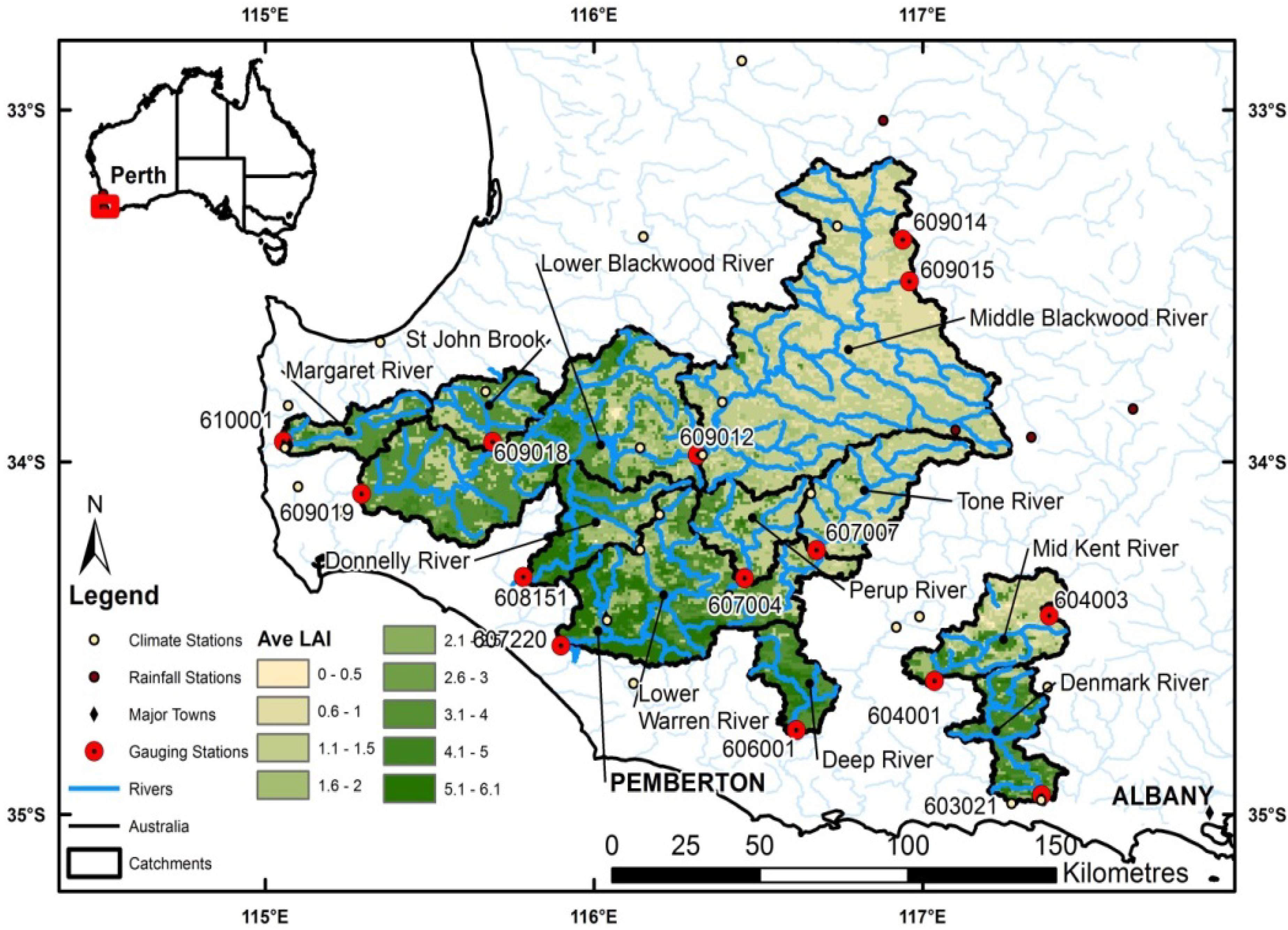
The study was undertaken on eleven gauged catchments with areas exceeding 440 km² in South-west Western Australia, spanning the 540–1200 mm rainfall zone (Figure 1).

Figure 1. Location of study catchments in South-west Western Australia.

Figure 1. Location of study catchments in South-west Western Australia.

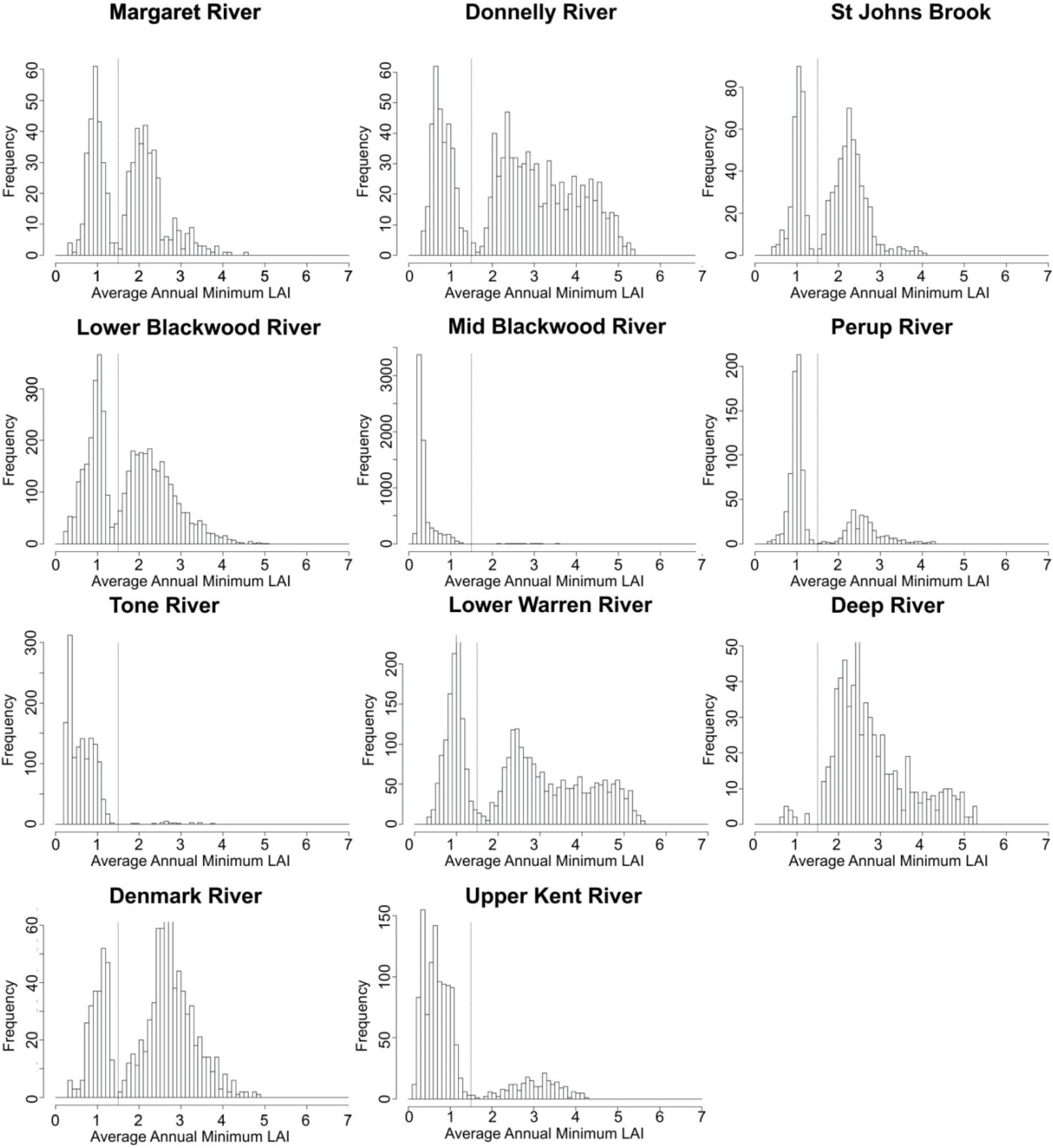
Study catchment characteristics are summarized in Table 1. Percent clearing (Table 1) was calculated using mean annual minimum Leaf Area Index (LAI) on a 1 km² grid derived from the improved (2011) MOD16 Global Terrestrial Data Set [26,27]. Average annual minimum LAI was calculated by taking the minimum LAI value in each water year (April to March) and averaging across the period April 2000 to March 2011. Use of minimum annual LAI gives a clear distinction between annual (predominantly grassland) and perennial (forest) vegetation, as illustrated in Figure 2. Note that in this region cleared land is mostly converted to grassland pasture in the >600 mm rainfall zone.

Table 1. Characteristics of the study catchments.

Study Catchment		Area (km2)	Percent Forest	Mean Annual Rain (mm) (2000–2011)	Mean Annual Runoff (mm) (2000–2011)	Penman Eo (mm)
1	Margaret River	443	58.0	790	114.5	1575
2	Donnelly River	787	70.0	862	77.6	1610
3	St Johns Brook	575	62.0	800	44.9	1575
4	Lower Blackwood River	3066	58.0	730	45.0	1591
5	Middle Blackwood River	5043	01.0	535	31.7	1610
6	Perup River	666	29.0	628	09.0	1591
7	Tone River	1015	02.0	593	32.5	1610
8	Lower Warren River	2187	64.0	867	54.7	1591
9	Deep River	467	98.0	994	51.2	1511
10	Denmark River	671	72.0	891	50.1	1526
11	Mid Kent River	880	18.0	591	17.8	1610

Table 1. Characteristics of the study catchments.

Study Catchment		Area (km2)	Percent Forest	Mean Annual Rain (mm) (2000–2011)	Mean Annual Runoff (mm) (2000–2011)	Penman Eo (mm)
1	Margaret River	443	58.0	790	114.5	1575
2	Donnelly River	787	70.0	862	77.6	1610
3	St Johns Brook	575	62.0	800	44.9	1575
4	Lower Blackwood River	3066	58.0	730	45.0	1591
5	Middle Blackwood River	5043	01.0	535	31.7	1610
6	Perup River	666	29.0	628	09.0	1591
7	Tone River	1015	02.0	593	32.5	1610
8	Lower Warren River	2187	64.0	867	54.7	1591
9	Deep River	467	98.0	994	51.2	1511
10	Denmark River	671	72.0	891	50.1	1526
11	Mid Kent River	880	18.0	591	17.8	1610

For three of the catchments (Warren River, Blackwood River and Kent River), we excised reach data (Figure 1). By using three gauging stations on the Warren River (two cleared upstream tributaries (West Australian Department of Water (DoW) Stations: 607004 and 607007) and one downstream (DoW Station: 607220)), we calculated mean annual runoff (mm) from available flow data [28] for the more heavily forested downstream area only. Similarly, for the Blackwood River we deducted the mid-catchment flow (DoW Station: 609012) and St John’s Brook (DoW Station: 609018) from the downstream gauge at (DoW Station: 609019) to isolate the more heavily forested lower section of this catchment. The mid Kent River reach was also excised between (Dow Station: 604001) and (Dow Station: 604003). This provided a dataset of eleven discharge records across a range of land clearing from 2% to 99%.

Annual rainfall data for open stations in this region were converted into a spatial dataset via regularised splines, produced at the same 1 km² grid as the MODIS LAI product. Locations of climate and rainfall stations within the study region are shown on Figure 1.

For each catchment the average annual rainfall over the study period 2000–2011 was analysed by sampling and then “binning” and averaging of point raster values using automated Python scripts utilizing the ArcGIS10 GeoProcessor Toolbox. Penman potential ET was averaged for each catchment using data from Donohue et al. [16]. We chose to average annual (water year runoff) from January 2000–November 2010 as it coincided with the available MODIS record and because there was no significant decline in rainfall across the study catchments over this period [29].

Figure 2. Separation of land use in each catchment into ‘forest’ (LAI > 1.5) and ‘grassland (LAI < 1.5) using MODIS minimum annual average LAI values (2000–2011).

Figure 2. Separation of land use in each catchment into ‘forest’ (LAI > 1.5) and ‘grassland (LAI < 1.5) using MODIS minimum annual average LAI values (2000–2011).

4. Results and Discussion

The optimal value of Choudhury’s n parameter was estimated for each of the eleven runoff records using Equation (5). Catchment average Z_e values were then calculated from Equation (8), with (range 0.10–0.13) estimated from regional soil hydrology groups documented by Moore et al. [30] and (range 4.5–8.0) from [16].

For this region, the average catchment value of Z_e is influenced by both the fraction of uncleared land and the aridity. In Table 2, catchments are ranked in order of percent forest cover (highest to lowest) and then average Z_e values and climate indices are presented for each catchment, together with the n, κ and α values used in the calculation of Z_e.

Table 2. Physical and model parameters for the study catchments.

Study Catchment	Percent Forest	Climate Index, ϕ (Eo/P)	n1	κ (cm3/cm−3)	α (mm)	Average Ze2 (mm)
Deep River	98.0	1.52	3.68	0.13	6.0	676
Denmark River	72.0	1.71	3.10	0.12	6.0	595
Donnelly River	70.0	1.87	2.28	0.12	7.8	520
Lower Warren River	64.0	1.83	2.71	0.13	6.2	479
St Johns Brook	62.0	1.97	2.65	0.12	6.0	489
Lower Blackwood River	58.0	2.18	2.35	0.12	8.0	556
Margaret River	58.0	2.00	1.71	0.10	7.5	396
Perup River	29.0	2.53	3.25	0.12	5.2	547
Mid Kent River	18.0	2.72	2.52	0.13	4.5	316
Tone River	02.0	2.72	2.08	0.12	4.6	270
Middle Blackwood River	01.0	3.00	1.90	0.13	6.0	287

Notes: ¹ Equation (5); ² Equation (8).

Table 2. Physical and model parameters for the study catchments.

Study Catchment	Percent Forest	Climate Index, ϕ (Eo/P)	n1	κ (cm3/cm−3)	α (mm)	Average Ze2 (mm)
Deep River	98.0	1.52	3.68	0.13	6.0	676
Denmark River	72.0	1.71	3.10	0.12	6.0	595
Donnelly River	70.0	1.87	2.28	0.12	7.8	520
Lower Warren River	64.0	1.83	2.71	0.13	6.2	479
St Johns Brook	62.0	1.97	2.65	0.12	6.0	489
Lower Blackwood River	58.0	2.18	2.35	0.12	8.0	556
Margaret River	58.0	2.00	1.71	0.10	7.5	396
Perup River	29.0	2.53	3.25	0.12	5.2	547
Mid Kent River	18.0	2.72	2.52	0.13	4.5	316
Tone River	02.0	2.72	2.08	0.12	4.6	270
Middle Blackwood River	01.0	3.00	1.90	0.13	6.0	287

Notes: ¹ Equation (5); ² Equation (8).

It is clear from Table 2 that forest clearing has been greatest in the drier catchments. The three catchments with less than 20% forest cover are in a zone with climate indices between 2.72 and 3.0. The mean Z_e of 291 mm for these catchments could reasonably be taken as a value for ‘grassland’ in this aridity zone. Conversely, the three catchments with 70% or more forest cover are much less arid and have a mean Z_e of 597 mm. However, the highest Z_e value (676 mm) is obtained for the catchment with the least (2%) clearing.

To investigate in more detail the how the effective root depths of grassland and forest might change with increasing aridity we used the physiologically-based model of Guswa [18].

Guswa Z values were obtained for grassland and forest using Equation (9), with the parameter values required to estimate A in Equation (11) taken from Donohue et al. [16]. The following values were common for grassland and forests: γ_r 0.5; D_r 0.1; L_r 1500. Values for W_ph and f_s were 0.22 and 0.8 for grassland and 0.33 and 1.0 for forest.

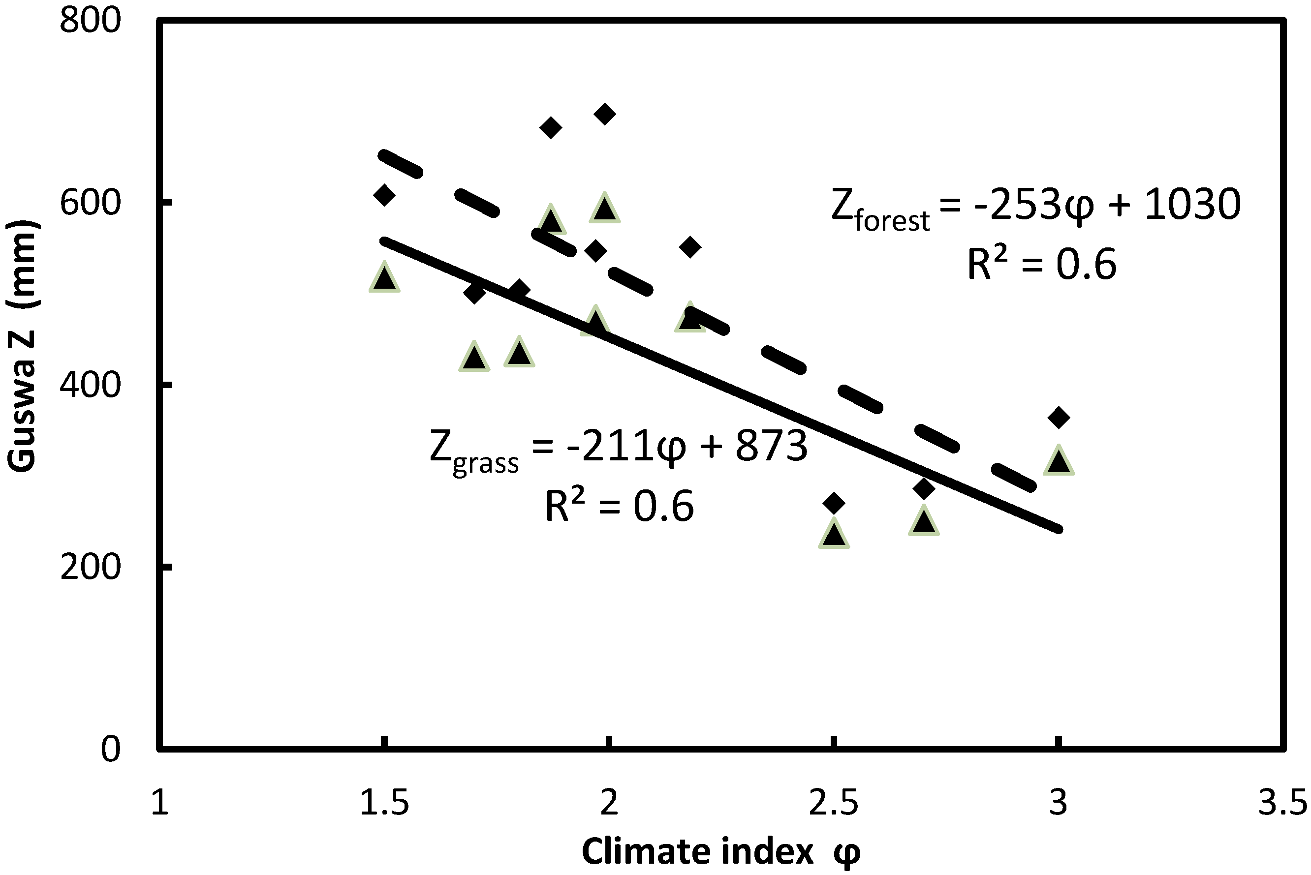
Estimates of the Guswa Z values for forest (Z_forest) and grassland (Z_grass), across each of the eleven catchments, show a clear trend of declining Z values with increasing aridity (Figure 3). The average ‘grassland’ Guswa Z value for the three driest catchments is 269 mm, with is remarkably close to the mean Z_e value of 291 mm. Using the regression relations in Figure 3 we calculate that at ϕ of 1.5, the Guswa Z for forest is 650 mm, which again compares favourably to the Z_e value for Deep river in Table 2 (676 mm). If we consider a ‘mix’ of 70% forest and 30% grassland for catchments with an aridity index of 1.8, then from the regression relations in Figure 3 we obtain a catchment average Guswa Z of (0.7 × 575) + (0.3 × 493) = 550 mm. Again, this compares well with the average Z_e from Table 2 for the Denmark, Donnelly and Lower Warren rivers (531 mm).

Figure 3. Z_forest (♦) and Z_grass (▲) calculated from the Guswa model for each catchment plotted against the climate index (ϕ = E_o/P).

Figure 3. Z_forest (♦) and Z_grass (▲) calculated from the Guswa model for each catchment plotted against the climate index (ϕ = E_o/P).

The decline in Z_forest with increasing aridity shown in Figure 3 also has implications for forest response to forecasted increased aridity across this region in the next 50 years. It is also evident from Figure 3 that the difference between Guswa Z values for forest and grassland diminishes with increasing aridity. At a climate index of about 1.5–2.0 the difference is 80 to 100 mm but from climate indices of 2.5–3.0 the difference has diminished to 30 to 35 mm.

4.1. Estimation of Runoff Using Guswa-Based and Choudhury ‘Default’ Models

Catchment average Guswa Z (Z_ave) values can be obtained from

Z_ave = (Z_forestF_forest + Z_grassF_grass)

(12)

where F_grass and F_forest are the fractions of the catchment under grass and forest.

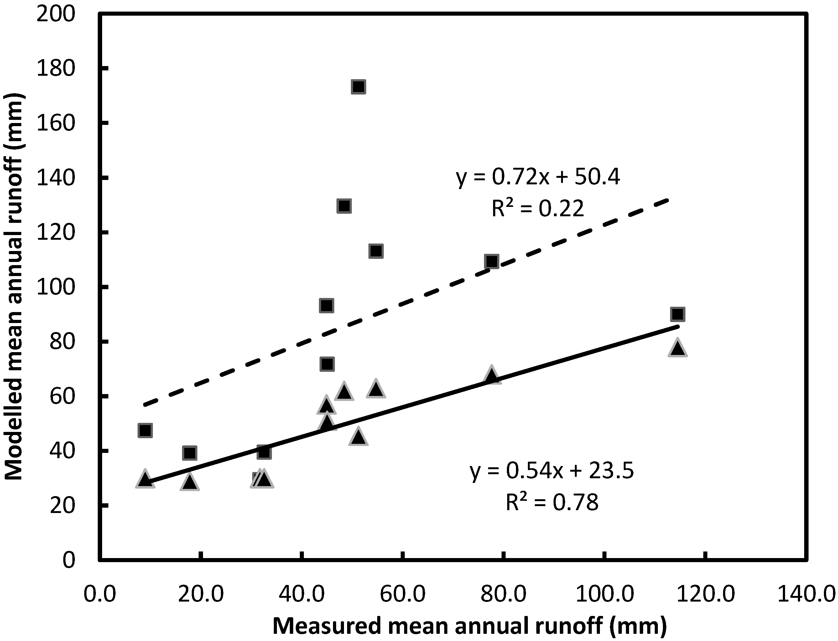
The resulting average Guswa Z values can then be used to independently estimate the Choudhury ‘n’ parameter for each catchment from Equation (7) and provide an estimate of catchment runoff without any calibration using Equation (5). This approach is shown in Figure 4 and is compared to the Choudhury ‘default’ model (n = 1.9). The runoff estimates that include an average rooting depth from the Guswa model are generally much closer to the observed mean annual runoff (2000–2011) than the Choudhury ‘default’ model. Note that catchments with less than 40 mm measured mean annual runoff are predominantly cleared (<30% forest cover) but have the most arid climate indices. For catchments with 40 mm to 80 mm measured mean annual runoff the forest cover ranges from 58% to 90% and the estimation of Guswa Z_forest to give catchment Z_ave values (Equation (12)) results in ‘n’ values that more accurately describe the runoff than the ‘default’ case. Root Mean Square Error is reduced from 21.0 (Choudhury ‘default’ model) to 7.5 (Guswa-based model). Bias is also reduced from 563.0 to 58.9. Weighted by catchment area over all eleven catchments the Guswa-based model overestimates regional mean annual runoff by 12% whereas the Choudhury ‘default’ model overestimates by 82%.

Figure 4. Comparison of runoff estimated from the Guswa-based model (▲) and Choudhury ‘default’ model (■) for eleven catchments in south-west Western Australia.

Figure 4. Comparison of runoff estimated from the Guswa-based model (▲) and Choudhury ‘default’ model (■) for eleven catchments in south-west Western Australia.

4.2. Implications for Climate Change

Within 400 km of the coast of south-west Western Australia the temperature is projected to increase in the range of 0.4 to 5.4 °C by 2080 and rainfall is projected to decrease by 0% to 80% [31], with a likely doubling of drought frequency [32]. Increasing temperature should lead to an increase in potential evapotranspiration but this has been countered by a decrease in global windspeed [33].

If there is no feedback between effective rooting depth and climate (and assuming κ and α remain constant), then for the model used here, the only effect on runoff will be rainfall decline and the ‘n’ parameter in Equation (5) remains unchanged. However, if effective rooting depth decreases with increasing aridity then ‘n’ will be altered (Equation (7)).

As an example, if we consider a 40% decline in rainfall over the forested Deep river catchment then holding ‘n’ constant leads to a decline in runoff from 51.2 mm (2000–2011 annual mean) to 5.2 mm. However, noting that a 40% decline in rainfall increases the aridity index to 2.53 allows ‘n’ to be adjusted in equation 7 by altering Z_e for the new aridity (climate index of 2.53) using the regression relation in Figure 3. The adjusted model Z_e is now 390 mm, giving an ‘n’ value of 2.37 and a reduction in the projected runoff decline to 25.8 mm (50% decline as opposed to 90% decline without feedback).

A decline in effective rooting depth with increasing aridity was demonstrated by Donohue et al. [16] for the Murray-Darling Basin in eastern Australia. If this climate-dependency follows the Guswa model projections then runoff decline is mitigated considerably when compared to the constant effective root depth case.

This simple example does not of course factor in any possible changes to the occurrence-intensity distribution of rainfall but illustrates the need for greater consideration of vegetation feedbacks when considering future runoff scenarios that may result from climate change.

5. Conclusions

We have shown that Choudhury’s ‘default’ model with n = 1.9 requires modification in order to describe mean annual runoff from catchments in south-west Western Australia. By using Donohue et al.’s [16] approach of incorporating three process-based ecohydrologic variables (effective rooting depth, mean storm depth and soil water storage capacity) into the description of n we were able to improve runoff prediction and gain insight into the effect of land use on runoff generation. The average effective rooting depth in a catchment was strongly correlated with the fraction of uncleared land identified using MODIS minimum annual average LAI values (2000–2011). Using the Guswa model to obtain values of Z for forest and grasslands that varied with catchment aridity gave an entirely uncalibrated model of mean annual runoff that overestimated the regional mean annual runoff by only 12%.

If effective rooting depth declines with increasing aridity then ‘n’ will decrease and water yields will be higher than if ‘n’ remains constant. However, ‘n’ is also affected by mean storm depth and so an understanding of how this is likely to change with declining rainfall is also important for improved understanding of how climate change could impact on water yields.