
Sensitivity Analysis of Flow and Temperature Distributions of Density Currents in a River-Reservoir System under Upstream Releases with Different Durations


Abstract
:1. Introduction
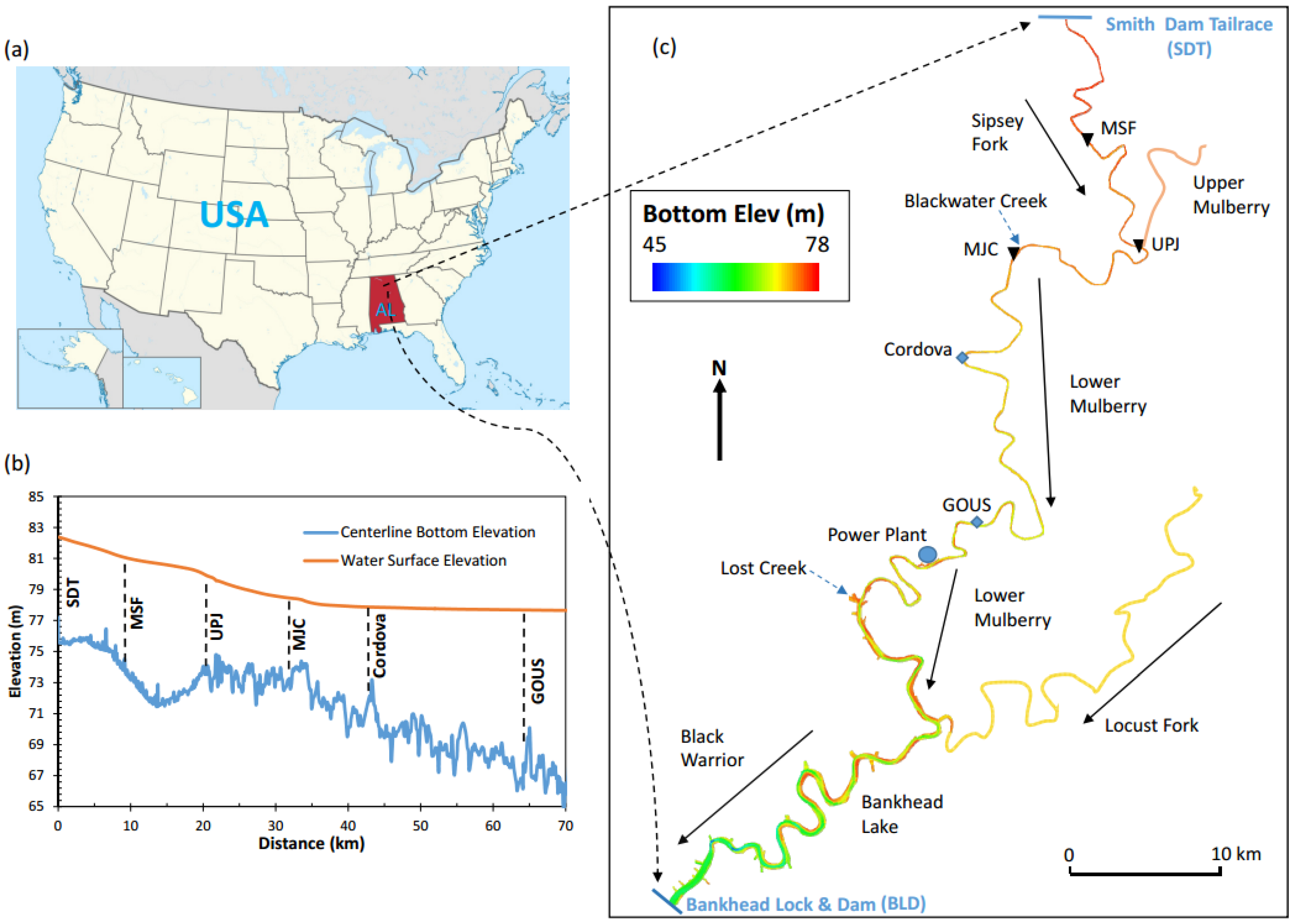
2. Study Area


| Abbreviation | Description |
|---|---|
| BLD | Bankhead Lock & Dam (downstream boundary of EFDC model) |
| Cordova | USGS 1 monitoring station at Cordova on the lower Mulberry River |
| GOUS | Monitoring station upstream the power plant |
| MSF | Middle cross section of Sipsey Fork |
| MJC | Middle cross section between the junction and Cordova |
| SDT | Smith Dam tailrace (upstream boundary of EFDC model) |
| UPJ | Just upstream of the junction of Sipsey Fork and the upper Mulberry Fork |
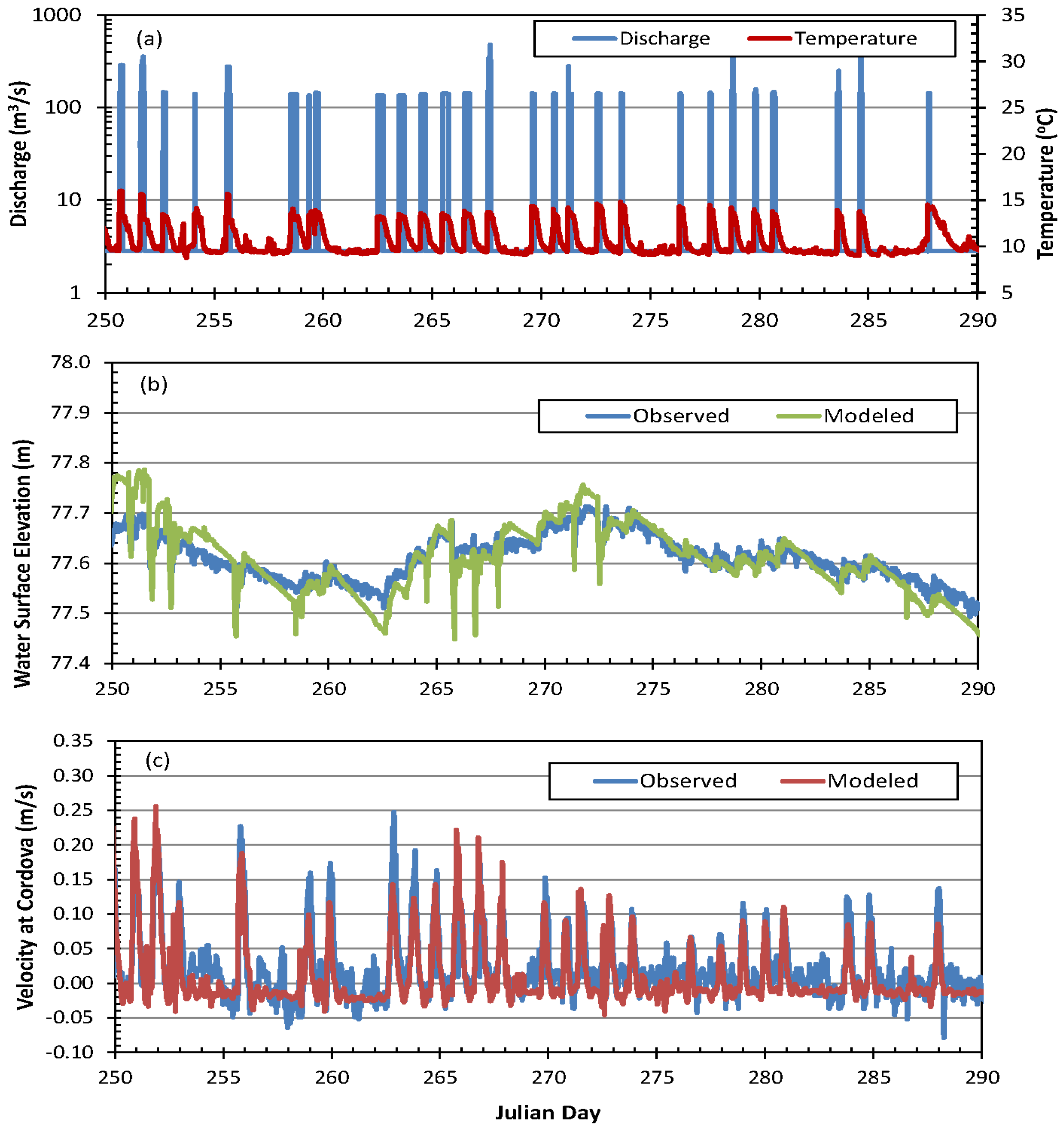
3. Model Application, Boundary Conditions, and Calibration Results

4. Model Scenarios
5. Results and Discussion
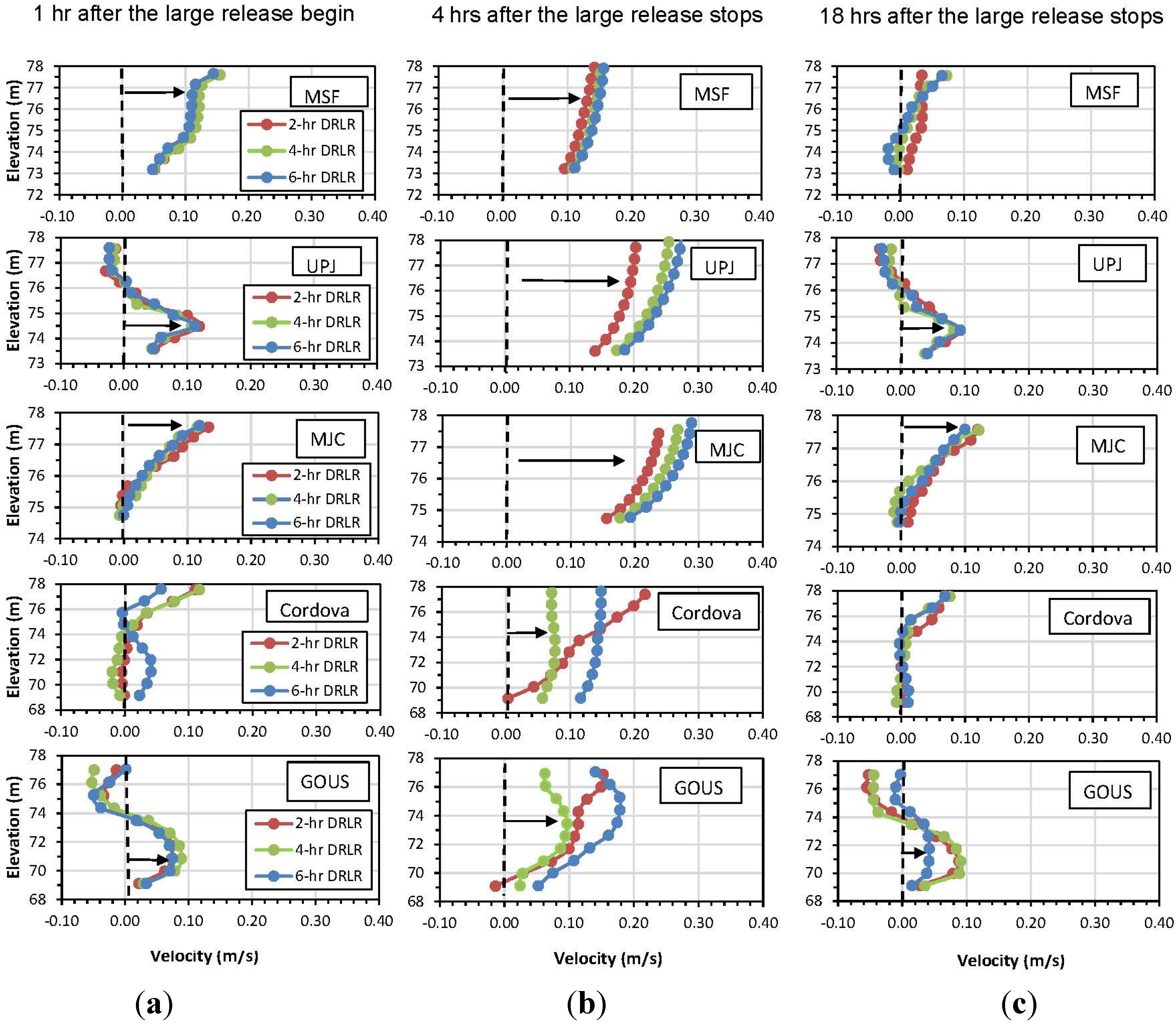
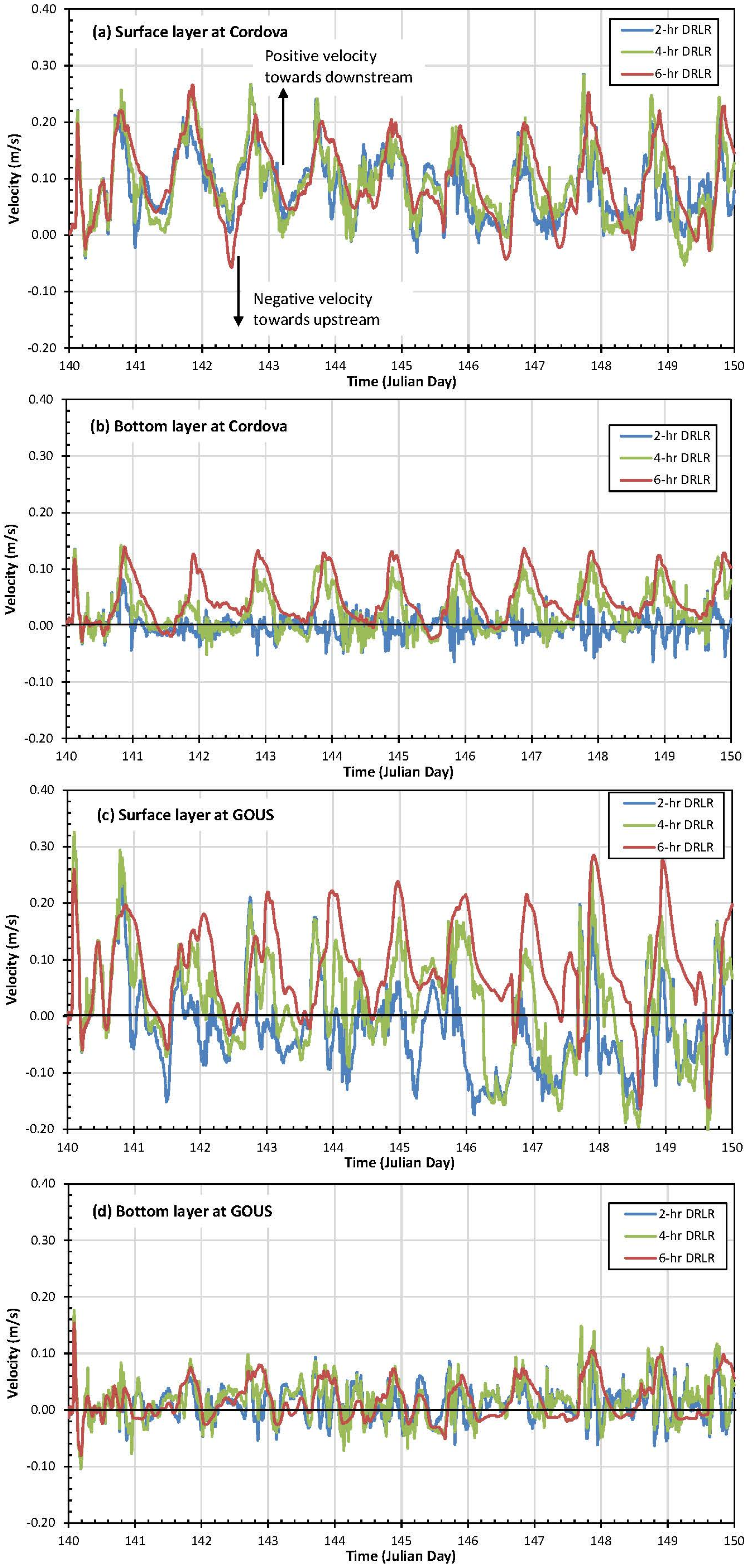
5.1. Velocity Distributions


| Location | Release | Layer | Maximum | Average | Deviation | Percent Hours 2 |
|---|---|---|---|---|---|---|
| Cordova | 2-h DRLR | Surface | 0.283 (−0.041) 1 | 0.085 (−0.010) | 0.055 (0.011) | 97.4% (2.6%) |
| Bottom | 0.135 (−0.064) | 0.017 (−0.013) | 0.018 (0.012) | 48.1% (51.9%) | ||
| 4-h DRLR | Surface | 0.282 (−0.053) | 0.093 (−0.017) | 0.060 (0.015) | 95.2% (4.8%) | |
| Bottom | 0.142 (−0.052) | 0.042 (−0.012) | 0.033 (0.010) | 69.0% (31.0%) | ||
| 6-h DRLR | Surface | 0.266 (−0.057) | 0.104 (−0.021) | 0.061 (0.015) | 93.0% (7.0%) | |
| Bottom | 0.139 (−0.028) | 0.053 (−0.011) | 0.038 (0.007) | 91.1% (8.9%) | ||
| GOUS | 2-h DRLR | Surface | 0.325 (−0.176) | 0.072 (−0.065) | 0.066 (0.043) | 33.1% (66.9%) |
| Bottom | 0.172 (−0.104) | 0.029 (−0.021) | 0.023 (0.016) | 62.2% (37.8%) | ||
| 4-h DRLR | Surface | 0.326 (−0.212) | 0.085 (−0.069) | 0.057 (0.052) | 58.5% (41.5%) | |
| Bottom | 0.174 (−0.103) | 0.034 (−0.022) | 0.027 (0.017) | 69.1% (30.9%) | ||
| 6-h DRLR | Surface | 0.285 (−0.164) | 0.106 (−0.037) | 0.068 (0.041) | 84.8% (15.2%) | |
| Bottom | 0.151 (−0.081) | 0.038 (−0.015) | 0.027 (0.011) | 60.9% (39.1%) |
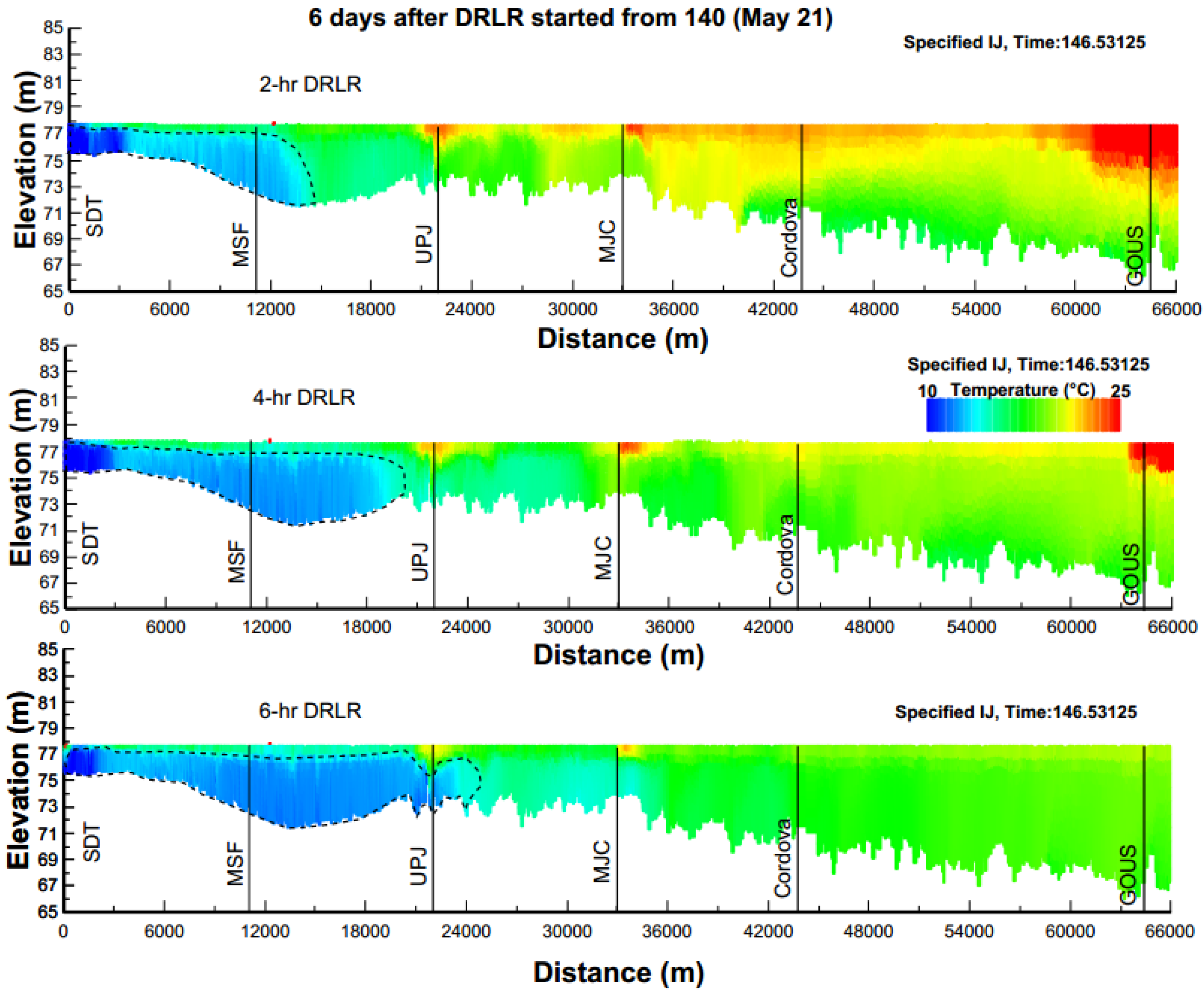
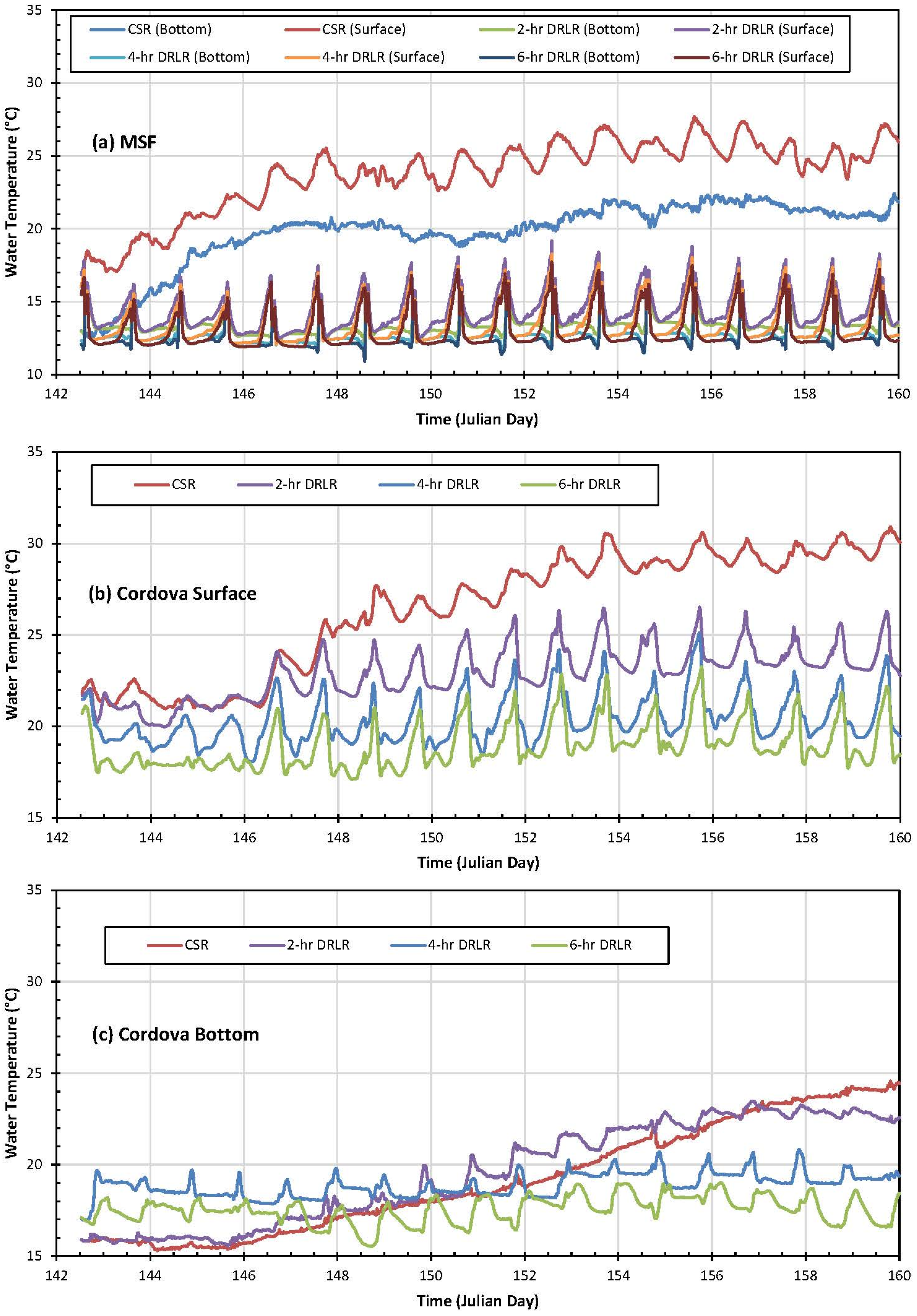
5.2. Temperature Distributions
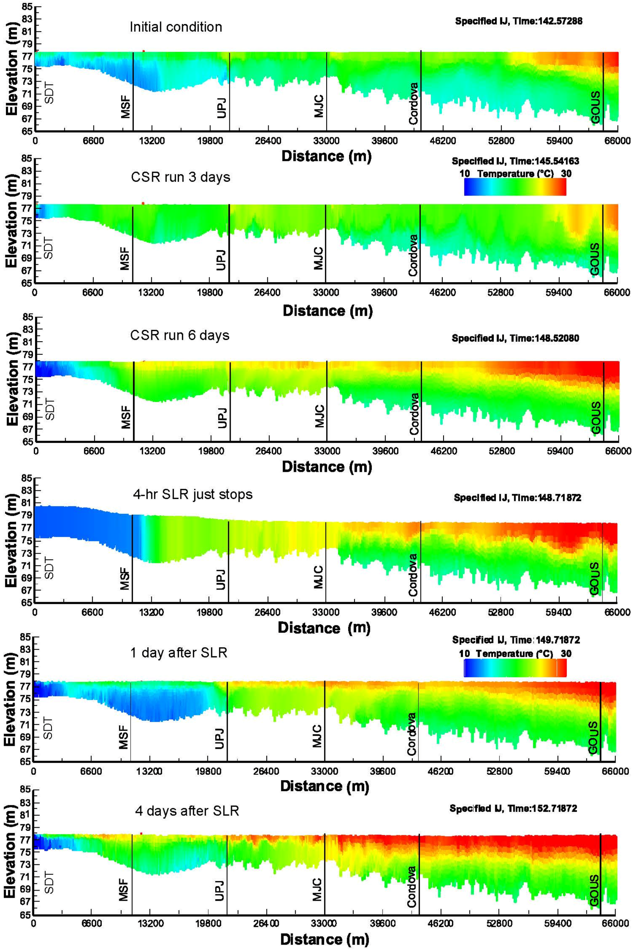
5.2.1. Single Large Release


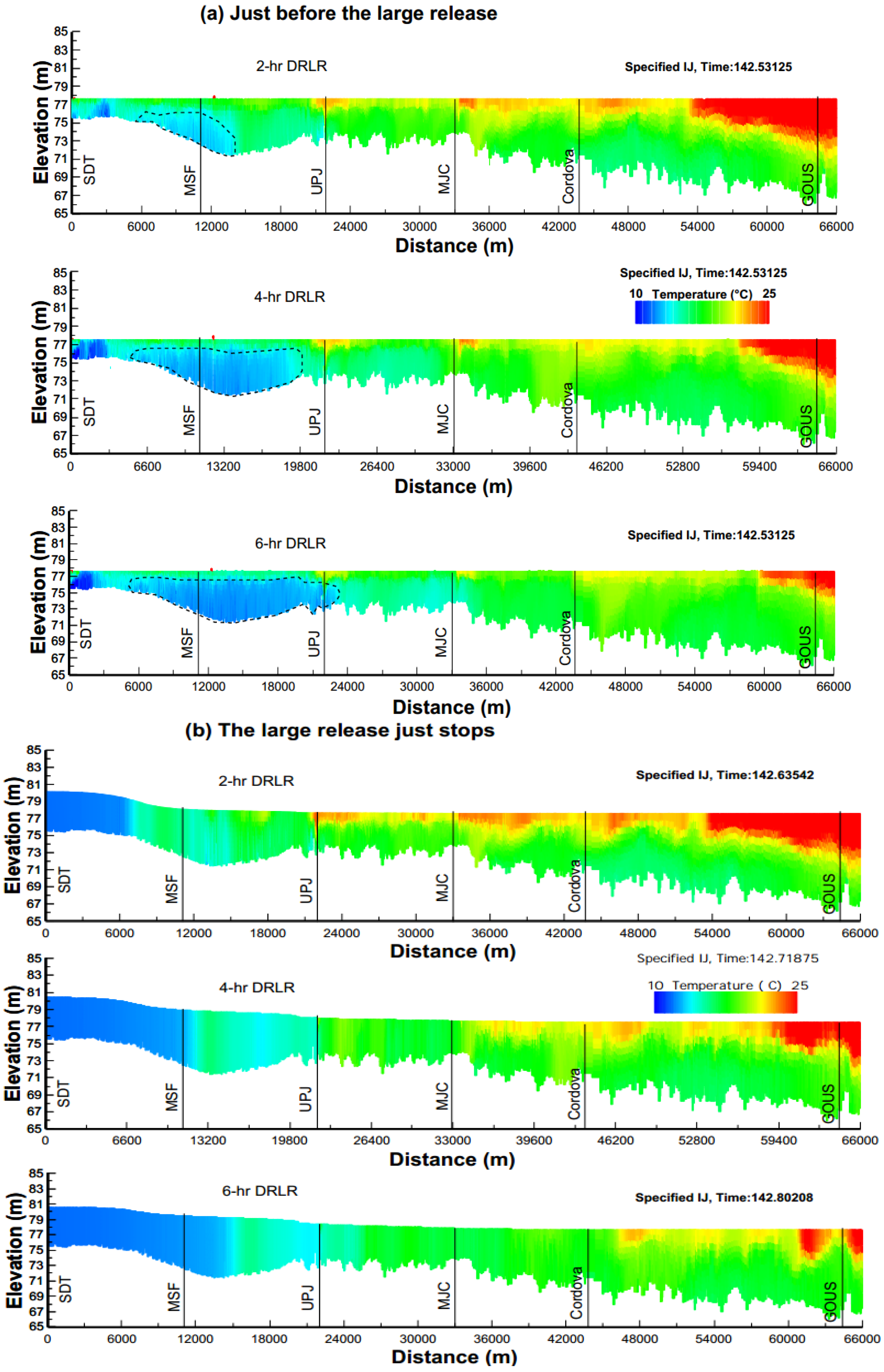
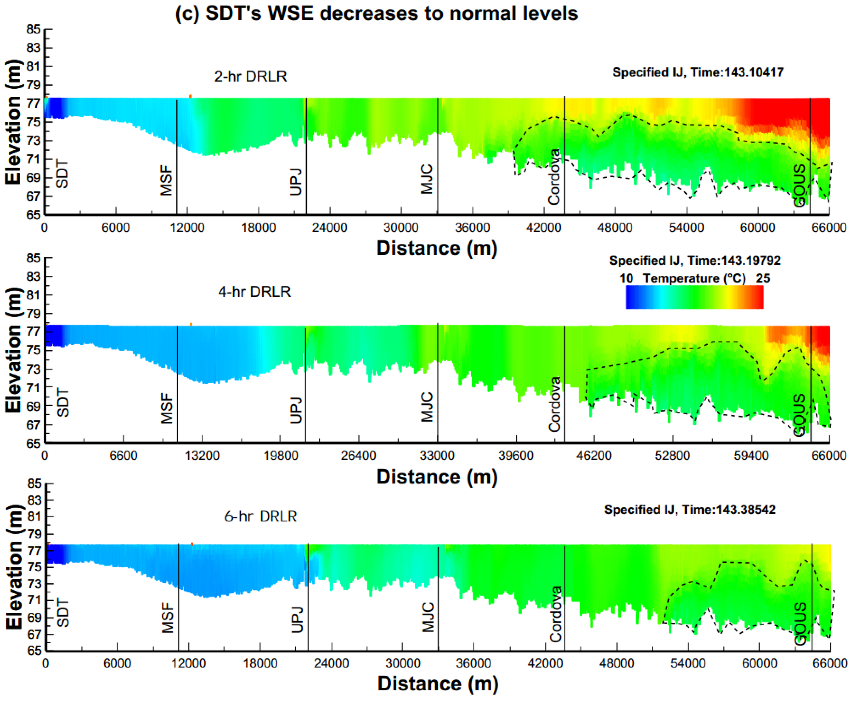
5.2.2. Daily Repeated Large Releases


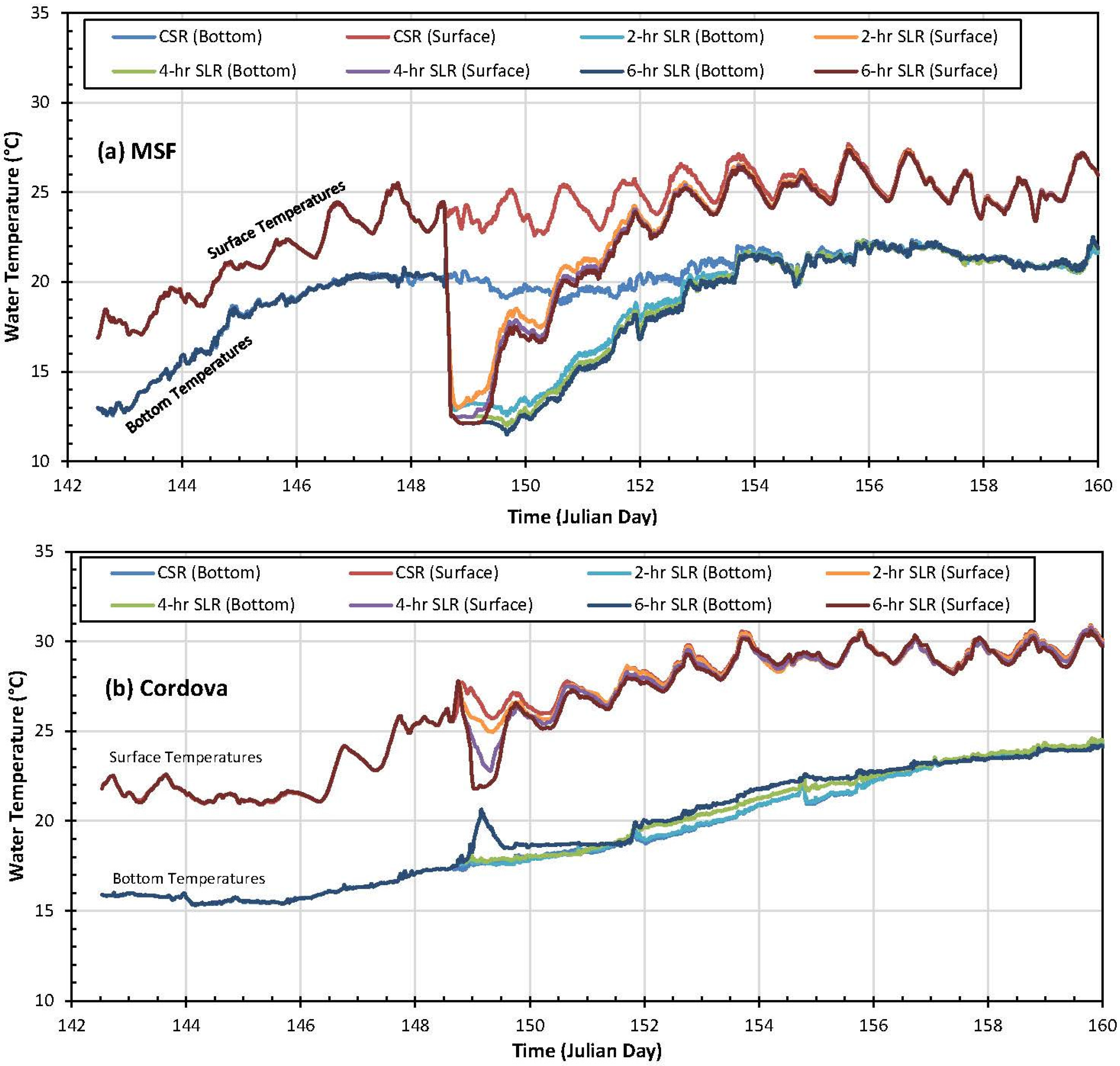
5.2.3. Comparison between CSR and DRLR
| Location | Release Type | Difference (Surface–Bottom) (°C) | |||
|---|---|---|---|---|---|
| Maximum | Minimum | Average | Deviation | ||
| MSF | CSR | 6.60 | 1.71 | 3.99 | 1.08 |
| 2-h DRLR | 6.60 | −0.02 | 0.94 | 1.32 | |
| 4-h DRLR | 6.35 | −0.01 | 0.76 | 1.32 | |
| 6-h DRLR | 5.72 | −0.01 | 0.65 | 1.26 | |
| Cordova | CSR | 10.44 | 4.96 | 7.26 | 1.43 |
| 2-h DRLR | 7.51 | −0.01 | 3.35 | 2.02 | |
| 4-h DRLR | 6.07 | −0.01 | 1.47 | 1.37 | |
| 6-h DRLR | 5.61 | −0.01 | 1.38 | 1.51 | |
| GOUS | CSR | 14.62 | 9.20 | 12.45 | 0.97 |
| 2-h DRLR | 13.63 | 6.66 | 11.33 | 1.35 | |
| 4-h DRLR | 12.24 | 1.88 | 8.53 | 2.40 | |
| 6-h DRLR | 10.79 | 0.58 | 4.71 | 2.69 | |
| Location | Temp Difference | Maximum | Minimum | Average | Deviation |
|---|---|---|---|---|---|
| MSF (Surface) | 2-h DRLR-CSR | 0.23 | −13.72 | −9.35 | 2.49 |
| 4-h DRLR-CSR | −0.41 | −14.65 | −10.25 | 2.56 | |
| 6-h DRLR-CSR | −0.92 | −14.67 | −10.63 | 2.53 | |
| Cordova (Surface) | 2-h DRLR-CSR | 0.36 | −7.35 | −3.53 | 2.24 |
| 4-h DRLR-CSR | −0.33 | −10.82 | −6.10 | 2.84 | |
| 6-h DRLR-CSR | −1.01 | −12.63 | −7.53 | 2.76 | |
| GOUS (Surface) | 2-h DRLR-CSR | 0.67 | −3.90 | −1.49 | 0.70 |
| 4-h DRLR-CSR | −0.55 | −9.43 | −4.29 | 1.65 | |
| 6-h DRLR-CSR | −1.56 | −12.91 | −8.84 | 2.20 | |
| MSF (Bottom) | 2-h DRLR-CSR | 3.53 | −9.23 | −6.30 | 2.39 |
| 4-h DRLR-CSR | 3.00 | −9.95 | −7.01 | 2.35 | |
| 6-h DRLR-CSR | 2.75 | −10.23 | −7.29 | 2.34 | |
| Cordova (Bottom) | 2-h DRLR-CSR | 2.19 | −2.08 | 0.38 | 0.81 |
| 4-h DRLR-CSR | 3.98 | −5.11 | −0.30 | 2.63 | |
| 6-h DRLR-CSR | 2.72 | −7.98 | −1.64 | 2.86 | |
| GOUS (Bottom) | 2-h DRLR-CSR | 1.20 | −2.88 | −0.38 | 0.70 |
| 4-h DRLR-CSR | 1.06 | −2.95 | −0.38 | 0.90 | |
| 6-h DRLR-CSR | 0.54 | −4.48 | −1.10 | 1.17 |
6. Conclusions
Acknowledgments
Author Contributions
Conflicts of Interest
References
- Serruya, S. The mixing patterns of the jordan river in lake kinneret. Limnol. Oceanogr. 1974, 19, 175–181. [Google Scholar] [CrossRef]
- Smith, P.C. A streamtube model for bottom boundary currents in the ocean. Deep Sea Res. Oceanogr. Abstr. 1975, 12, 853–873. [Google Scholar] [CrossRef]
- Carmack, E.C.; Gray, C.B.; Pharo, C.H.; Daley, R.J. Importance of lake-river interaction on seasonal patterns in the general circulation of kamloops lake, british columbia. Limnol. Oceanogr. 1979, 24, 634–644. [Google Scholar] [CrossRef]
- Fischer, H.B.; Smith, R.D. Observations of transport to surface waters from a plunging inflow to lake mead 1. Limnol. Oceanogr. 1983, 28, 253–272. [Google Scholar] [CrossRef]
- Alavian, V.; Ostrowski, P., Jr. Use of density current to modify thermal structure of tva reservoirs. J. Hydraul. Eng. 1992, 118, 688–706. [Google Scholar] [CrossRef]
- Chikita, K. The role of sediment-laden underflows in lake sedimentation: Glacier-fed peyto lake, canada. J. Fac. Sci. Hokkaido Univ. Ser. VII Geophys. 1992, 9, 211–224. [Google Scholar]
- Akiyama, J.; Stefan, H.G. Plunging flow into a reservoir: Theory. J. Hydraul. Eng. ASCE 1984, 110, 484–499. [Google Scholar] [CrossRef]
- Hauenstein, W.; Dracos, T. Investigation of plunging density currents generated by inflows in lakes. J. Hydraul. Res. 1984, 22, 157–179. [Google Scholar] [CrossRef]
- Alavian, V. Behavior of density currents on an incline. J. Hydraul. Eng. 1986, 112, 27–42. [Google Scholar] [CrossRef]
- Singh, B.; Shah, C. Plunging phenomenon of density currents in reservoirs. Houille Blanche 1971, 1, 59–64. [Google Scholar] [CrossRef]
- Savage, S.; Brimberg, J. Analysis of plunging phenomena in water reservoirs. J. Hydraul. Res. 1975, 13, 187–205. [Google Scholar] [CrossRef]
- Denton, R. Density current inflows to run of the river reservoirs. In Proceedings of the 21st IAHR World Congress, Melbourne, Australia, 13–18 August 1985.
- Kranenburg, C. Gravity current fronts advancing into horizontal ambient flow. J. Hydraul. Eng. 1993, 119, 369–379. [Google Scholar] [CrossRef]
- Fang, X.; Stefan, H.G. Dependence of dilution of a plunging discharge over a sloping bottom on inflow conditions and bottom friction. J. Hydraul. Res. 2000, 38, 15–25. [Google Scholar] [CrossRef]
- Cortés, A.; Rueda, F.; Wells, M. Experimental observations of the splitting of a gravity current at a density step in a stratified water body. J. Geophys. Res. Oceans 2014, 119, 1038–1053. [Google Scholar] [CrossRef]
- Imberger, J.; Patterson, J. Dynamic reservoir simulation model-dyresm: 5. In Transport Models for Inland and Coastal Waters; Academic Press: New York, NY, USA, 1981; pp. 310–361. [Google Scholar]
- Buchak, E.M. Simulation of a Density Underflow into Wellington Reservoir Using Longitudinal-Vertical Numerical Hydrodynamics; JE Edinger Associates: Washington, DC, USA, 1984. [Google Scholar]
- Jokela, J.; Patterson, J. Quasi-two-dimensional modelling of reservoir inflow. In Proceedings of the 21st Congress, International Association for Hydraulic Research, Melbourne, Australia, 19–23 August 1985.
- Gu, R.R. Impact of inflow and ambient conditions on density-induced current in a stratified reservoir. Mod. Phys. Lett. B 2009, 23, 429–432. [Google Scholar] [CrossRef]
- Cole, T.M.; Wells, S.A. CE-QUAL-W2: A Two-Dimensional, Laerally Averaged, Hydrodynamic and Water Quality Model; U.S. Army Engineering and Research Development Center: Vicksburg, MS, USA, 2010. [Google Scholar]
- Farrell, G.J.; Stefan, H.G. Buoyancy Induced Plunging Flow into Reservoirs and Costal Regions; Anthony Falls Hydraulics Laboratory: Minneapolis, MN, USA, 1986. [Google Scholar]
- Fukushima, Y.; Watanabe, M. Numerical simulation of density underflow by the k-ε turbulence model. J. Hydrosci. Hydr. Eng. 1990, 8, 31–40. [Google Scholar] [CrossRef]
- Bournet, P.; Dartus, D.; Tassin, B.; Vincon-Leite, B. Numerical investigation of plunging density current. J. Hydraul. Eng. 1999, 125, 584–594. [Google Scholar] [CrossRef]
- Soliman, M.; Ushijima, S.; Kantouch, S. Density current propagation in a tidal river. In River Flow 2014; CRC Press: Boca Raton, FL, USA, 2014. [Google Scholar]
- Shlychkov, V.A.; Krylova, A.I. A numerical model of density currents in estuaries of siberian rivers. Numer. Anal. Appl. 2014, 7, 255–261. [Google Scholar] [CrossRef]
- Imran, J.; Islam, M.A.; Huang, H.; Kassem, A.; Dickerson, J.; Pirmez, C.; Parker, G. Helical flow couplets in submarine gravity underflows. Geology 2007, 35, 659–662. [Google Scholar] [CrossRef]
- An, S.; Julien, P.Y. Three-dimensional modeling of turbid density currents in Imha Reservoir, South Korea. J. Hydraul. Eng. 2014, 140. [Google Scholar] [CrossRef]
- Firoozabadi, B.; Afshin, H.; Aram, E. Three-dimensional modeling of density current in a straight channel. J. Hydraul. Eng. 2009, 135, 393–402. [Google Scholar] [CrossRef]
- Hamrick, J.M.; Mills, W.B. Analysis of water temperatures in conowingo pond as influenced by the peach bottom atomic power plant thermal discharge. Environ. Sci. Policy 2000, 3, 197–209. [Google Scholar] [CrossRef]
- Kulis, P.; Hodges, B.R. Modeling gravity currents in shallow bays using a sigma coordinate model. In Proceedings of the 7th International Conference on Hydroscience ann Enginnering, Philadelphia, PA, USA, 10–13 September 2006.
- Liu, X.; Garcia, M.H. Numerical simulation of density current in Chicago river using environmental fluid dynamics code (EFDC). In Proceedings of World Environmental & Water Resource Congress, Honolulu, HI, USA, 12–16 May 2008.
- Xie, R.; Wu, D.-A.; Yan, Y.-X.; Zhou, H. Fine silt particle pathline of dredging sediment in the yangtze river deepwater navigation channel based on efdc model. J. Hydrodyn. Ser. B 2010, 22, 760–772. [Google Scholar] [CrossRef]
- Lyubimova, T.; Lepikhin, A.; Konovalov, V.; Parshakova, Y.; Tiunov, A. Formation of the density currents in the zone of confluence of two rivers. J. Hydrol. 2014, 508, 328–342. [Google Scholar] [CrossRef]
- Do An, S. Three-dimensional numerical simulation of intrusive density currents. J. Environ. Sci. Int. 2014, 23, 1223–1232. [Google Scholar] [CrossRef]
- Hirt, C.; Nichols, B. Flow-3D User’s Manual; Flow Science Inc.: Santa Fe, NM, USA, 1988. [Google Scholar]
- Fatih, Ü.; Varcin, H. Investigation of plunging depth and density currents in eğrekkaya dam reservoir. Teknik Dergi 2012, 23, 5725–5750. [Google Scholar]
- Wells, M.; Nadarajah, P. The intrusion depth of density currents flowing into stratified water bodies. J. Phys. Oceanogr. 2009, 39, 1935–1947. [Google Scholar] [CrossRef]
- Biton, E.; Silverman, J.; Gildor, H. Observations and modeling of a pulsating density current. Geophys. Res. Lett. 2008, 35. [Google Scholar] [CrossRef]
- Owens, E.M.; Effler, S.W.; Prestigiacomo, A.R.; Matthews, D.A.; O’Donnell, S.M. Observations and modeling of stream plunging in an urban lake. J. Am. Water Resour. Assoc. 2012, 48, 707–721. [Google Scholar] [CrossRef]
- Hodges, B.; Dallimore, C. Estuary, Lake and Coastal Ocean Model: Elcom; Science Manual; Centre of Water Research, University of Western Australia: Perth, Australia, 2006. [Google Scholar]
- Cook, C.B.; Richmond, M.C. Monitoring and simulating 3-D density currents at the confluence of the snake and clearwater rivers. In Critical Transitions in Water And Environmental Resources Management; American Society of Civil Engineers (ASCE): Salt Lake City, UT, USA, 2004. [Google Scholar]
- Jackson, P.R.; García, C.M.; Oberg, K.A.; Johnson, K.K.; García, M.H. Density currents in the chicago river: Characterization, effects on water quality, and potential sources. Sci. Total Environ. 2008, 401, 130–143. [Google Scholar] [CrossRef] [PubMed]
- Chen, G.; Fang, X.; Devkota, J. Understanding Flow Dynamics and Density Currents in a River-Reservoir System under Upstream Reservoir Releases. Avaliable online: http://www.tandfonline.com/doi/abs/10.1080/02626667.2015.1112902 (accessed on 27 October 2015).
- Hamrick, J.M. A Three-dimensional Environmental Fluid Dynamics Code: Theoritical and Computational Aspects; Virginia Institute of Marine Science: Gloucester Point, VA, USA, 1992. [Google Scholar]
- Shen, J.; Lin, J. Modeling study of the influences of tide and stratification on age of water in the tidal james river. Estuar. Coast. Shelf Sci. 2006, 68, 101–112. [Google Scholar] [CrossRef]
- Jeong, S.; Yeon, K.; Hur, Y.; Oh, K. Salinity intrusion characteristics analysis using EFDC model in the downstream of geum river. J. Environ. Sci. 2010, 22, 934–939. [Google Scholar] [CrossRef]
- Kim, C.-K.; Park, K. A modeling study of water and salt exchange for a micro-tidal, stratified northern gulf of mexico estuary. J. Mar. Syst. 2012, 96–97, 103–115. [Google Scholar] [CrossRef]
- Devkota, J.; Fang, X. Numerical Simulation of Flow Dynamics in a Tidal River Under Various Upstream Hydrologic Conditions. Avaliable online: http://www.tandfonline.com/doi/pdf/10.1080/02626667.2014.947989 (accessed on 27 August 2015).
- Wang, Y.; Shen, J.; He, Q. A numerical model study of the transport timescale and change of estuarine circulation due to waterway constructions in the Changjiang estuary, China. J. Mar. Syst. 2010, 82, 154–170. [Google Scholar] [CrossRef]
- Caliskan, A.; Elci, S. Effects of selective withdrawal on hydrodynamics of a stratified reservoir. Water Resour. Manag. 2009, 23, 1257–1273. [Google Scholar] [CrossRef]
- Mellor, G.L.; Yamada, T. Development of a turbulence closure model for geophysical fluid problems. Rev. Geophys. Space Phys. 1982, 20, 851–875. [Google Scholar] [CrossRef]
- Fang, X.; Weems, T.B.; Devkota, J.; Chen, G. Watershed Modeling, Water Balance Analysis, Three-Dimensional Flow and Thermal Discharge Modeling for the William C. Gorgas Plant; Department of Civil Engineering: Auburn, AL, USA, 2013. [Google Scholar]
- Craig, P.M. User’s Manual for EFDC_Explorer 7: A Pre/Post Processor for the Environmental Fluid Dynamics Code; Dynamic Solutions-International, LLC: Edmonds, WA, USA, 2012. [Google Scholar]
- Harlow, F.H. The Particle-in-Cell Method for Numerical Solution of Problems in Fluid Dynamics; Los Alamos Scientific Lab.: Los Alamos, NM, USA, 1962. [Google Scholar]
- Ahlstrom, S.; Foote, H.; Arnett, R.; Cole, C.; Serne, R. Multicomponent Mass Transport Model: Theory and Numerical Implementation (Discrete-Parcel-Random-Walk Version); Battelle Pacific Northwest Labs.: Richland, WA, USA, 1977. [Google Scholar]
- Abrahams, A.D.; Parsons, A.J.; Luk, S.H. Field measurement of the velocity of overland flow using dye tracing. Earth Surf. Process. Landf. 1986, 11, 653–657. [Google Scholar] [CrossRef]
- Guo-Qing, H.; Yuan-Jie, D.; Hui, W.; Xian-Kui, Q.; Yan-Hua, W. Laboratory testing of magnetic tracers for soil erosion measurement. Pedosphere 2011, 21, 328–338. [Google Scholar] [CrossRef]
© 2015 by the authors; licensee MDPI, Basel, Switzerland. This article is an open access article distributed under the terms and conditions of the Creative Commons Attribution license (http://creativecommons.org/licenses/by/4.0/).
Share and Cite
Chen, G.; Fang, X. Sensitivity Analysis of Flow and Temperature Distributions of Density Currents in a River-Reservoir System under Upstream Releases with Different Durations. Water 2015, 7, 6244-6268. https://doi.org/10.3390/w7116244
Chen G, Fang X. Sensitivity Analysis of Flow and Temperature Distributions of Density Currents in a River-Reservoir System under Upstream Releases with Different Durations. Water. 2015; 7(11):6244-6268. https://doi.org/10.3390/w7116244
Chicago/Turabian StyleChen, Gang, and Xing Fang. 2015. "Sensitivity Analysis of Flow and Temperature Distributions of Density Currents in a River-Reservoir System under Upstream Releases with Different Durations" Water 7, no. 11: 6244-6268. https://doi.org/10.3390/w7116244