Optimizing Water Allocation under Uncertain System Conditions for Water and Agriculture Future Scenarios in Alfeios River Basin (Greece)—Part B: Fuzzy-Boundary Intervals Combined with Multi-Stage Stochastic Programming Model

Abstract

Optimal water allocation within a river basin still remains a great modeling challenge for engineers due to various hydrosystem complexities, parameter uncertainties and their interactions. Conventional deterministic optimization approaches have given their place to stochastic, fuzzy and interval-parameter programming approaches and their hybrid combinations for overcoming these difficulties. In many countries, including Mediterranean countries, water resources management is characterized by uncertain, imprecise and limited data because of the absence of permanent measuring systems, inefficient river monitoring and fragmentation of authority responsibilities. A fuzzy-boundary-interval linear programming methodology developed by Li et al. (2010) is selected and applied in the Alfeios river basin (Greece) for optimal water allocation under uncertain system conditions. This methodology combines an ordinary multi-stage stochastic programming with uncertainties expressed as fuzzy-boundary intervals. Upper- and lower-bound solution intervals for optimized water allocation targets and probabilistic water allocations and shortages are estimated under a baseline scenario and four water and agricultural policy future scenarios for an optimistic and a pessimistic attitude of the decision makers. In this work, the uncertainty of the random water inflows is incorporated through the simultaneous generation of stochastic equal-probability hydrologic scenarios at various inflow positions instead of using a scenario-tree approach in the original methodology.

1. Introduction

Optimal water allocation of a river basin poses great challenges for engineers due to various uncertainties associated with the hydrosystem, its parameters and its impact factors as well as their interactions. These uncertainties are often associated with various complexities in terms of information quality [1]. The random characteristics of natural processes (i.e., precipitation and climate change) and stream conditions (i.e., stream inflow, water supply, storage capacity, and river-quality requirement), the errors in estimated modeling parameters (i.e., benefit and cost parameters), and the vagueness of system objectives and constraints are all possible sources of uncertainties. These uncertainties may exist in both left- and right-hand sides of the constraints as well as coefficients of the objective function. Some uncertainties may be expressed as random variables. At the same time, some random events can only be quantified as discrete intervals with fuzzy boundaries, leading to multiple uncertainties presented as different formats in the system's components [2]. Traditional optimization techniques can embody various characteristics but only as deterministic values. In various real-world problems, results generated by these traditional optimization techniques could be rendered highly questionable if the modeling inputs could not be expressed with precision [1,3,4]. For these reasons conventional deterministic optimization approaches have given their place to stochastic (SP), fuzzy (FP) and interval-parameter programming (IPP) approaches and their hybrid combinations in order to face up these difficulties. Various methodologies have been developed and proposed [4,5,6,7,8,9,10,11,12,13,14,15,16] in order to embody in optimal water allocation uncertainties of various influencing factors and hydrosystem characteristics.

SP can handle uncertainties expressed as random variables with known probability distributions and at the same time connect efficiently the pre-regulated policies and the associated economic implications caused by improper policies [2]. Reference [17] introduced a stochastic dynamic programming model for a single reservoir deriving optimal reservoir operating policies subject to reliability constraints. Reference [18] presented a stochastic optimization approach for a multi-reservoir planning with hydropower system under uncertainty. They assigned a given probability to each of a range of inputs occurring at different stages of an optimization horizon. A common SP method is the two-stage stochastic programming (TSP). It is based on the concept of recourse, expressed as the ability to take corrective actions after a random event has occurred. The initial action is called the first-stage decision, and the corrective one is named the recourse decision. The first-stage decisions have to be made before further information of initial system uncertainties is revealed, whereas the recourse decisions are allowed to adapt to this information [19]. Reference [6] developed an inexact two-stage stochastic programming method for water resources management, dealing with uncertainties expressed as both probability distributions and intervals and accounting for economic penalties due to infeasibility. Reference [20] proposed a scenario-based multistage stochastic programming model for water supplies planning from highland lakes. A number of inflow scenarios are explicitly taken into account in order to determine a contract for water delivery in the coming year. In general, multistage stochastic programming (MSP) approach permitted modified decisions in each time stage based on the real-time realizations of uncertain system conditions [8,21].

SP cannot handle randomness in the right-hand-side parameters. However, chance-constrained programming (CCP) method can deal with this type of uncertainty. It can reflect the reliability of satisfying (or risk of violating) system constraints under uncertainty [22,23]. Reference [24] used a CCP model for reservoir systems planning of irrigation districts. Reference [23] developed an inexact CCP method for assessing risk of violating system constraints, in which uncertainties are expressed as probabilities and intervals. Reference [25] presented a mathematical programming model for the reservoir capacity planning under random stream inflows. Based on the CCP method it considers a special target-priority policy based on given system reliabilities. Reference [26] developed a stochastic model for optimal multi-period operation of a multi-reservoir system for a basin operating under a conjunctive use of ground and surface water framework, with uncertainties in the inflows dealt using CCP method. However, TSP and CCP have difficulties in dealing with uncertain parameters when their probabilistic distributions are not available [13]. Moreover, the increased data requirements for specifying the parameters’ probability distributions may affect their practical applicability [1].

Uncertainties may be also related to the incompleteness or impreciseness of observed information [27]. This type of uncertainty, expressed as fuzziness, cannot be handled by SP but by fuzzy programming (FZ). FZ can deal with decision problems under fuzzy goal and constraints and ambiguous and vague coefficients not only in the objective function but also in the constraints [28,29]. Reference [30] used FZ method in order to optimize a multi-reservoir system, expressing the uncertainties in reservoir inflows as fuzzy sets. Reference [31] introduced a fuzzy compromise approach for water resources planning under imprecision uncertainty. Reference [32] proposed an interactive fuzzy approach for planning a stream water resources management system including vague and imprecise information. Reference [1] proposed a multistage fuzzy-stochastic programming model for water-resources allocation and management with uncertainties expressed as probability distributions and fuzzy sets.

Interval parameter programming (IPP) can handle uncertain parameters expressed as intervals with known lower- and upper-bounds, without any distributional information that is always required in fuzzy and stochastic programming [33]. However, in many real-world problems, the lower- and upper-bounds of some interval parameters can rarely be acquired as deterministic values [10,11]. Instead, they may often be provided as subjective information and therefore defined as fuzzy sets. This drives to dual uncertainties that cannot be addressed through the conventional IPP and FP methods. Hybrid approaches that link IPP with FP have been proposed for handling this combined type of complexities. However, these combined approaches have difficulties in tackling uncertainties expressed as random variables [34]. Additionally, a linkage to economic consequences of violated policies preregulated by authorities through taking recourse actions in order to correct any infeasibility is missing.

Therefore, in case of multiple uncertainties expressed at various and complex formats, one possible approach is to build hybrid modeling techniques combining IPP, FP and SP. In [12], a violation analysis approach has been developed for planning water resources management system associated with uncertain information, based on a fuzzy multistage stochastic integer programming model within a scenario-based frame. However, by using such a scenario-based approach, the resulting multistage programming model could become too large when all water-availability scenarios are considered. In [1], a multistage fuzzy-stochastic programming method has been developed dealing with uncertainties presented as fuzzy sets and probability distributions by employing vertex analysis and generating of a set of representative scenarios within a multistage context. The same problem due to the scenario-based approach is also here identified. Reference [13] developed a two-stage fuzzy-stochastic programming method for planning water resources allocation of agricultural irrigation systems. Also in this case a scenario-based approach sets limitations when the study system is very large and complicated. In reference [14], a method is developed for tackling multiple uncertainties through integration of stochastic dynamic programming, fuzzy-Markov chain, vertex analysis and factorial analysis techniques. It may have, though, computational (among others) difficulties to handle many other uncertain parameters (such as interval or dual-probabilities) that exist in large-scale practical problems. In [15], an optimal water allocation method is proposed incorporating techniques of interval-parameter programming and fuzzy vertex analysis within a fixed-mix stochastic programming framework to deal with uncertainties presented as probability distributions and dual intervals. In this study, only one reservoir is considered for all subareas and crops, in order to enable the use of linear programming method. Reference [16] presented an interval-fuzzy De Novo programming method for planning water-resources management systems under uncertainty, mainly useful for designing an optimal system rather than optimizing a given system.

In the present work, an optimal water allocation method under uncertain system conditions is explored for the Alfeios river basin in Greece. Alfeios is a water resources system of great natural, ecological, social and economic importance for Western Greece, since it has the longest watercourse and highest flow rate in the Peloponnese region [35,36,37]. The main water user in the basin is irrigation, playing a vital social, economic and environmental role associated among others with agricultural income and with water, food and energy efficiency. The other water-use sectors are hydropower generation and drinking water supply. As analyzed in [38], in Alfeios river basin, as in most Mediterranean countries, water resources management has been focused up to now on an essentially supply-driven approach. Authority responsibility relationships are fragmented and law enforcement and policy implementation are weak, facts that lead to the difficulty of gathering the necessary data for water resources management or even worst to data loss. In some cases, river monitoring, which is crucial for water quantity and quality assessment, if present, is either inefficient with intermittent periods with no measurements, or due to low financial means the monitoring programs are short and undertaken by a small number of personnel leading to unreliable or/and short-term data. In this case some sources of obtaining hydrologic, technical, economic and environmental data required for water resources management is by making additional periodic measuring expeditions, indirectly by expert knowledge, by informal knowledge by the local population, or by more general data concerning a wider geographical location (i.e., country level) from national, European or international databases. Data of this type with a high degree of uncertainty may be easily defined as fluctuation ranges, and therefore, simulated as intervals with lower- and upper-bounds, either as deterministic or fuzzy, without the need of any distributional or probabilistic information.

This work is the second part of two papers, both aiming at analyzing and applying two similar in terms of their basic concepts optimization techniques for optimal water allocation under uncertain system conditions in a real and complex multi-tributary and multi-period water resources system, the Alfeios river basin. The first method is an inexact two-stage stochastic programming (ITSP) as developed by [6]. The second methodology, described and discussed in this paper, extends the ITSP in order to take into account fuzzy instead of deterministic boundaries for the variables, which are expressed as intervals, since some intervals are fuzzy in nature. This fuzzy-boundary interval-stochastic programming (FBISP) method proposed by [2] is selected. This algorithmic process is advanced including two different solution methods in order to take into account different risk attitudes of decision makers concerning system uncertainties. In [2], the uncertain random information of the water inflow is modeled through a multi-layer scenario tree having the limitation of resulting in too large mathematical problem to be applied to large-scale real-world problems. Additionally, this approach is not capable to incorporate the persistence in hydrological records and to take into consideration conditional probabilities for quantifying water availability, which are important in many real-world cases. In this work, in order to overcome these difficulties, the system dynamics related to random water inflows are reflected through the consideration of the various equal-probability hydrologic scenarios that have been stochastically generated simultaneously at multiple sites of the river basin. A thorough description of this proposed change in the methodology of [2] is provided in Section 2.1.

The results obtained from this methodology include (a) the optimized water-allocation target with a minimized risk of economic penalty from shortages and opportunity loss from spills; and (b) an optimized water-allocation plan (identification of water allocation and shortages based on the optimized water allocation targets) with a maximized system benefit over a multi-period planning horizon. These types of results are derived as fuzzy-boundary intervals. The total net system benefits and the benefits and penalties of each main water uses for the Alfeios are studied and analyzed based on the application of the FBISP method for a baseline scenario and four water and agricultural future scenarios developed within the Sustainability of European Irrigated Agriculture under Water Framework Directive and Agenda 2000 (WADI) project [39,40,41,42]. These future scenarios cover various possible technical, environmental and socio-economics aspects of the future space for different European Union (EU) water and agricultural policies, having an impact mainly on agriculture and also on water resources management. Changes on crop patterns, yields, subsidies, farmer income, variable input costs, market prices per agricultural product, fertilizers, and water and hydropower prices are some of the variables described into the narratives of these scenarios, which in turn serve as inputs into the optimization algorithm for the evaluation and the estimation of their effect on the water allocation pattern and the system benefits. Finally, for applying the above mentioned optimal water allocation methodology, benefit analysis of each water use identifying the unit benefit and unit penalties of each m³ of water allocated to each one of the water uses has been undertaken for the Alfeios River in [38].

The paper is organized as follows: Section 2 includes the presentation of the mathematical background of the FBISP as provided in [2]. In Section 2.1, the limitations of the applied methodology and the proposed by this study changes are analyzed in details. Section 3 describes shortly the Alfeios river basin and the formulation of optimization problem for the Alfeios hydrosystem. The steps of this process and the used software programs are presented schematically in the form of a flow chart in Section 3.2. Section 4 analyzes in brief the WADI future scenarios. Section 5 presents the results and their interpretation and finally, Section 6 discussion and conclusions.

2. Mathematical Formulation of the FBISP Method

In the present work, a FBISP methodology as developed by [2,43,44] is employed for optimizing water allocation under uncertain system conditions in the Alfeios river basin in Greece. The used methodology is based on the combination of three optimization techniques: (a) the multistage-stochastic programming; (b) the fuzzy programming (employing the vertex analysis for fuzzy sets) and (c) the interval parameter programming. Each technique has a unique contribution in enhancing the model’s capability of incorporating uncertainty presented as multiple formats. Its theoretical and mathematical background of the model and its parameters is presented below based on [2], but for simplicity reason the terms, referring to the variables with negative coefficients, are not included into all equations and inequalities, since they are absent from the examined application to Alfeios river basin. The complete mathematical model including also these terms with negative coefficients can be found in [2].

In the FBISP model, assume that there is no intersection between the fuzzy sets at the two bounds (e.g., let $\widetilde{b_{rt}^{\pm }}= \left[\widetilde{b_{rt}^{-}}, \widetilde{b_{rt}^{+}}\right] = \left[\left[b_{rt}^{-}, \overline{b_{rt}^{-}}\right], \left[b_{rt}^{+}, \overline{b_{rt}^{+}}\right]\right]$, where $\widetilde{b_{rt}^{-} }$and $\widetilde{b_{rt}^{+}}$ are fuzzy lower- and upper-bounds of $\widetilde{b_{rt}^{\pm }}, b_{rt}^{-}$ and $\overline{b_{rt}^{-}}$are the lower- and upper-boundary of $\widetilde{b_{rt}^{-}}$;$b_{rt}^{+} and\overline{b_{rt}^{+}}$ are the lower-and upper-boundary of $\widetilde{b_{rt}^{+}}$). This is due to satisfy the definition of an interval value that its lower-bound should not be larger than its upper-bound [5]. Secondly, interval numbers are used to express uncertainties without distribution information. If the fuzzy sets of an interval’s lower- and upper- bounds intersect, then the so-called “interval” is actually described by fuzzy membership functions, such that the interval representation becomes unnecessary [45]. Thirdly, if the fuzzy sets of an interval’s lower- and upper-bound intersect, the interactive algorithm for solving the interval-parameter programming problem cannot be used for solving such a FBISP model.

Then, two solution methods are proposed for solving the FBISP model, which are based on an optimistic and pessimistic approach of the uncertainties by the decision makers, respectively. In the first solution methods (i.e., optimistic or risk-prone), a set of submodels corresponding to $\widetilde{f^{+}}$ can be first formulated based on the interactive algorithm; for each $\widetilde{f^{+}}$ submodel, take one end point from each of the fuzzy intervals (i.e., [$\underset{\_}{c_{jt}^{+}}$, $\overline{c_{jt}^{+}}$], [$\underset{\_}{d_{jtk}^{-}}$, $\overline{d_{jtk}^{-}}$] and [ $\underset{\_}{b_{rt}^{+}}$, $\overline{b_{rt}^{+}}$]); then, the obtained end points can be combined into an n-array, leading to $2^n$ combinations for n fuzzy sets [9,46]. Through solving $2^n$ problems, a set of upper-bound objective-function values $(f_1^{+},f_2^{+},\dots ,f_{2^n}^{+})$ can be obtained. In detail, for each α-cut level, a set of $\widetilde{f^{+}}$ submodels can be formulated as follows (assume that the right-hand sides and objective are both greater than zero):

$$Max \widetilde{f^{+}} = {\displaystyle \sum }_{t = 1}^T\left\{{\displaystyle \sum }_{j = 1}^{j_1}\left[\left[\underset{\_}{c_{jt}^{+}, } \overline{c_{jt}^{+}}\right]+ c_{jt}^{+}\right] x_{jt}^{+}\right\}- {\displaystyle \sum }_{t = 1}^T{\displaystyle \sum }_{k = 1}^{K_r}{p}_{tk}\left\{{\displaystyle \sum }_{j = 1}^{j_2}\left[\left[\underset{\_}{d_{jtk}^{-}, } \overline{d_{jtk}^{-}}\right]+ d_{jtk}^{-}\right]y_{jtk}^{-}\right\}$$

(1)

subject to:

$${{\displaystyle \sum }}_{j = 1}^{j_1}\left[\left|\underset{\_}{a_{rjt}^{-}}\right|Sign\left(\underset{\_}{a_{rjt}^{-}}\right), \left|\overline{a_{rjt}^{-}}\right|Sign\left(\overline{a_{rjt}^{-}}\right) \right]x_{jt}^{+} \le [\underset{\_}{b_{rt}^{+}},\overline{b_{rt}^{+}}],\forall r,t$$

(2)

$$\begin{gathered} {\displaystyle \sum }_{j = 1}^{j_1}\left|a_{ijt}^{-}\right|Sign\left(a_{ijt}^{-}\right)x_{jt}^{+} +{\displaystyle \sum }_{j = 1}^{j_2}\left[\left|\underset{\_}{{a^{\prime }}_{ijtk}^{+}}\right|Sign \left(\underset{\_}{{a^{\prime }}_{ijtk}^{+}}\right), \left|\overline{{a^{\prime }}_{ijtk}^{+}}\right|Sign\left(\overline{{a^{\prime }}_{ijtk}^{+}}\right)\right]y_{jtk}^{-} \ge \left[\underset{\_}{w_{itk}^{-}},\overline{w_{itk}^{-}}\right] \\ \forall t,k=1,2,\dots .,K_t \\ {x}_{jt}^{+}, y_{jtk}^{-} \ge 0 \end{gathered}$$

(3)

where $x_{jt}^{+}$ $\left(j = 1,2,\dots ., j_1\right)$ are upper-bounds of the first-stage decision variables ($x_{jt}^{\pm })$, and $y_{jtk}^{-}$ ($k = 1,2,\dots ., K_t and j = 1,2,\dots ., j_2)$ are lower-bounds of the recourse decision variables $\left(y_{jtk}^{\pm }\right)$.

Through solving $2^n$ submodels, a set of values ($f_1^{+}, f_2^{+}, \dots ,f_{2^n}^{+})$ can be obtained. Let $f_{opt}^{+}$ be the minimum value of the upper-bound (for the objective-function value) with $\underset{\_}{f_{opt}^{+}} = min\left(f_1^{+}, f_2^{+}, \dots ,f_{2^n}^{+}\right)$, and $\overline{f_{opt}^{+}}$ be the maximum value of the upper-bound with $\overline{f_{opt}^{+}} = min\left(f_1^{+}, f_2^{+}, \dots ,f_{2^n}^{+}\right)$. Then, the optimized upper-bound interval for the objective function value (under an α-cut level) can be identified as follows:

$${\left[\underset{\_}{f_{opt}^{+}},\overline{f_{opt}^{+}}\right]}^a = {\left[min\left(f_1^{+}, f_2^{+}, \dots ,f_{2^n}^{+}\right), max\left(f_1^{+}, f_2^{+}, \dots ,f_{2^n}^{+}\right)\right]}^a$$

(4)

Based on the solutions from the first set of submodels, submodels corresponding to $\widetilde{f^{-}}$ can be formulated as:

$$Max \widetilde{f^{-}} = {\displaystyle \sum }_{t = 1}^T\left\{{\displaystyle \sum }_{j = 1}^{j_1}\left[\left[\underset{\_}{c_{jt}^{-}, } \overline{c_{jt}^{-}}\right]+ c{\prime }_{jt}^{-}\right] x_{jt}^{-}\right\}- {\displaystyle \sum }_{t = 1}^T{\displaystyle \sum }_{k = 1}^{K_r}{p}_{tk}\left\{{\displaystyle \sum }_{j = 1}^{j_2}\left[\left[\underset{\_}{d_{jtk}^{+}, } \overline{d_{jtk}^{+}}\right]+ d{\prime }_{jtk}^{+}\right]y_{jtk}^{+}\right\}$$

(5)

subject to:

$${{\displaystyle \sum }}_{j = 1}^{j_r}\left[\left|\underset{\_}{a_{rjt}^{+}}\right|Sign\left(\underset{\_}{a_{rjt}^{+}}\right), \left|\overline{a_{rjt}^{+}}\right|Sign\left(\overline{a_{rjt}^{+}}\right) \right]x_{jt}^{-} \le [\underset{\_}{b_{rt}^{-}},\overline{b_{rt}^{-}}],\forall r,t$$

(6)

$$\begin{gathered} {{\displaystyle \sum }}_{j = 1}^{j_1}\left|a_{ijt}^{+}\right|Sign\left(a_{ijt}^{+}\right)x_{jt}^{-} +{{\displaystyle \sum }}_{j = 1}^{j2}\left[\left|\underset{\_}{{a^{\prime }}_{ijtk}^{-}}\right|Sign \left(\underset{\_}{{a^{\prime }}_{ijtk}^{-}}\right) , \left|\overline{{a^{\prime }}_{ijtk}^{-}}\right|Sign\left(\overline{{a^{\prime }}_{ijtk}^{-}}\right)\right]y_{jtk}^{+} \ge \left[\underset{\_}{w_{itk}^{+}}, \overline{w_{itk}^{+}}\right] ,\forall i,t;k = 1,2,\dots ., K_t \\ 0\le x_{jt}^{-} \le X_{jtopt}^{+} , \forall t;j = 1,2,\dots ,j_{t1} \\ {y}_{jtk}^{+} \ge y_{jtkopt}^{-} , \forall t;j = 1,2,\dots ,j_2, k = 1,2,\dots , K_t \end{gathered}$$

(7)

where $x_{jtopt}^{+}$ ($j=1,2,\dots ,j_1)$, $x_{jtopt}^{-}$ ($j=j_1+1,j_1+2,\dots ,j_1+n)$, $y_{jtkopt}^{-}$ ($j=1,2,\dots ,j_2)$ and $y_{jtkopt}^{+}$ ($j=j_2+1, j_2+2,\dots ,j_2+n_2)$, are solutions corresponding to $\underset{\_}{f_{opt}^{+}}$. Through solving $2^n$ deterministic problems, a set of values ($f_1^{-},f_2^{-},\dots ,f_{2n}^{-}$) can be obtained. The optimized lower-bound interval for the objective-function value (under an α-cut level) can be identified as follows:

$${\left[\underset{\_}{f_{opt}^{-}}, \overline{f_{opt}^{-}}\right]}^a = {\left[min\left(f_1^{-}, f_2^{-}, \dots ,f_{2^n}^{-}\right), max\left(f_1^{-}, f_2^{-}, \dots ,f_{2n}^{-}\right)\right]}^a$$

(8)

where $\underset{\_}{f_{opt}^{-}}$ is the minimum value of the lower-bound (for the objective function value) with $\underset{\_}{f_{opt}^{-}} = min\left(f_1^{-}, f_2^{-}, \dots ,f_{2^n}^{-}\right)$; $\overline{f_{opt}^{-}}$ is the maximum value of the lower-bound with $\overline{f_{opt}^{-}} = \max \left(f_1^{-}, f_2^{-}, \dots ,f_{2n}^{-}\right)$. Then, through integrating the computational results of the two sets of submodels, the solution for the objective function value (under an α-cut level) can be obtained. Iteratively, the computational process can be repeated with the other α-cut levels.

The above optimistic solution method identifies the solutions for the first-stage and recourse decisions variables by first solving the best-case submodel (i.e., upper-bound objective function value when the problem is to be maximized). This includes the upper-bound system solution for total benefit, which is associated with more advantageous (more favorable) conditions. In example, this is related to the upper-bound benefit coefficients, lower-bound cost coefficients, upper-bound reservoir capacities, lower-bound reserved storage requirements, etc. The resulting solution can provide intervals for the objective function value and decision variables, and can be easily interpreted for generating decision alternatives.

However, this solution method may provide a wide-ranging objective function value because significant (and costly) first-stage and recourse decisions are required under unfavorable conditions (represented by worst-case parameter values) [47]. Consequently, another solution method based on risk adverse is proposed for solving the FBISP model to reduce the interval width of the objective-function value, in which the worst-case submodel (i.e., corresponding to the lower-bound objective function) can be first solved to identify a more appropriate set of first-stage and recourse decision variables. In this case, the interval for the objective function value is narrower, but it may lead to increased opportunity loss, being incapable of achieving the highest benefit under advantageous conditions. Thus, we have:

$$Max \widetilde{f^{-}} = {\displaystyle \sum }_{t = 1}^T\left\{{\displaystyle \sum }_{j = 1}^{j_1}\left[\left[\underset{\_}{c_{jt}^{-}, } \overline{c_{jt}^{-}}\right]+ c{\prime }_{jt}^{-}\right] x_{jt}^{-}\right\}- {\displaystyle \sum }_{t = 1}^T{\displaystyle \sum }_{k = 1}^{K_r}{p}_{tk}\left\{{\displaystyle \sum }_{j = 1}^{j_2}\left[\left[\underset{\_}{d_{jtk}^{+}, } \overline{d_{jtk}^{+}}\right]+ d{\prime }_{jtk}^{+}\right]y_{jtk}^{+}\right\}$$

(9)

subject to:

$${{\displaystyle \sum }}_{j = 1}^{j_r}\left[\left|\underset{\_}{a_{rjt}^{+}}\right|Sign\left(\underset{\_}{a_{rjt}^{+}}\right), \left|\overline{a_{rjt}^{+}}\right|Sign\left(\overline{a_{rjt}^{+}}\right) \right]x_{jt}^{-} \le [\underset{\_}{b_{rt}^{-}}, \overline{b_{rt}^{-}}], \forall r,t$$

(10)

$${{\displaystyle \sum }}_{j = 1}^{j_1}\left|a_{ijt}^{+}\right|Sign\left(a_{ijt}^{+}\right)x_{jt}^{-} +{{\displaystyle \sum }}_{j = 1}^{j2}\left[\left|\underset{\_}{{a^{\prime }}_{ijtk}^{-}}\right|Sign \left(\underset{\_}{{a^{\prime }}_{ijtk}^{-}}\right), \left|\overline{{a^{\prime }}_{ijtk}^{-}}\right|Sign\left(\overline{{a^{\prime }}_{ijtk}^{-}}\right)\right]y_{jtk}^{+} \ge \left[\underset{\_}{w_{itk}^{+}}, \overline{w_{itk}^{+}}\right] , \forall i,t;k = 1,2,\dots ., K_t$$

(11)

Through solving $2^n$ deterministic problems, a set of values ($f_1^{-}, f_2^{-}, \dots ,f_{2n}^{-}$) can be obtained. The optimized lower-bound interval for the objective-function value (under an α-cut level) can be identified as follows:

$${\left[\underset{\_}{f_{opt}^{-}}, \overline{f_{opt}^{-}}\right]}^a = {\left[min\left(f_1^{-}, f_2^{-}, \dots ,f_{2^n}^{-}\right), max\left(f_1^{-}, f_2^{-}, \dots ,f_{2n}^{-}\right)\right]}^a$$

(12)

In the second solution method, characterized as risk adverse and corresponding to the worst-case solution, the previously described process is reversed so that the lower-bound submodels are solved first, and their solution is integrated into the upper-bound formulation of the problem, which is solved in the second step. Based on the solutions from the first set of submodels, submodels corresponding to $\widetilde{f^{+}}$ can be formulated as:

$$Max \widetilde{f^{+}} = {\displaystyle \sum }_{t = 1}^T\left\{{\displaystyle \sum }_{j = 1}^{j_1}\left[\left[\underset{\_}{c_{jt}^{+}, } \overline{c_{jt}^{+}}\right]+ c_{jt}^{+}\right] x_{jt}^{+}\right\}- {\displaystyle \sum }_{t = 1}^T{\displaystyle \sum }_{k = 1}^{K_r}{p}_{tk}\left\{{\displaystyle \sum }_{j = 1}^{j_2}\left[\left[\underset{\_}{d_{jtk}^{-}, } \overline{d_{jtk}^{-}}\right]+ d_{jtk}^{-}\right]y_{jtk}^{-}\right\}$$

(13)

subject to:

$${{\displaystyle \sum }}_{j = 1}^{j_1}\left[\left|\underset{\_}{a_{rjt}^{-}}\right|Sign\left(\underset{\_}{a_{rjt}^{-}}\right), \left|\overline{a_{rjt}^{-}}\right|Sign\left(\overline{a_{rjt}^{-}}\right) \right]x_{jt}^{+} \le [\underset{\_}{b_{rt}^{+}},\overline{b_{rt}^{+}}], \forall r,t$$

(14)

$$\begin{gathered} {{\displaystyle \sum }}_{j = 1}^{j_1}\left|a_{ijt}^{-}\right|Sign\left(a_{ijt}^{-}\right)x_{jt}^{+} +{{\displaystyle \sum }}_{j = 1}^{j_2}\left[\left|\underset{\_}{{a^{\prime }}_{ijtk}^{+}}\right|Sign \left(\underset{\_}{{a^{\prime }}_{ijtk}^{+}}\right) , \left|\overline{{a^{\prime }}_{ijtk}^{+}}\right|Sign\left(\overline{{a^{\prime }}_{ijtk}^{+}}\right)\right]y_{jtk}^{-} \ge \left[\underset{\_}{w_{itk}^{-}}, \overline{w_{itk}^{-}}\right] , \forall t,k = 1,2,\dots ., K_t \\ {x}_{jt}^{+} , y_{jtk}^{-} \ge 0 \\ {x}_{jt}^{+} \ge x_{jtopt}^{-}, \forall t;j = 1,2,\dots ,j_1 \\ 0\le y_{jtk}^{-} \le y_{jtkopt}^{+}, \forall t;j = 1,2,\dots ,j_2, k = 1,2,\dots , K_t \end{gathered}$$

(15)

where $x_{jtopt}^{-}$ ($j=1,2,\dots ,j_1)$, $y_{jtkopt}^{+}$ ($j=1,2,\dots ,j_2)$ are solutions corresponding $f_{opt}^{-}$.

Through solving $2^n$ submodels, a set of values ($f_1^{+}, f_2^{+}, \dots ,f_{2^n}^{+})$ can be obtained. Then, the optimized upper-bound interval for the objective function value (under an α-cut level) can be identified as follows:

$${\left[\underset{\_}{f_{opt}^{+}}, \overline{f_{opt}^{+}}\right]}^a = {\left[min\left(f_1^{+}, f_2^{+}, \dots ,f_{2^n}^{+}\right), max\left(f_1^{+}, f_2^{+}, \dots ,f_{2^n}^{+}\right)\right]}^a$$

(16)

Limitations of the Applied Methodology and Corresponding Changes

The main limitations of the chosen FBISP methodology as described in [2] are the following. The uncertain random information of the water inflow is modeled through a multi-layer scenario tree which is representative for the universe of water-availability conditions for the relative simple application of [2] including a hydro network with two tributaries and two reservoirs. With such a scenario-based approach, the resulting mathematical problem can become too large to be applied to large-scale real-world problems. The same problem has been mentioned among others in [12,13,14,15]. Moreover, the random variables (mainly the water inflows) are assumed to take on discrete distributions, such that the study can be solved through linear programming method. However, when water resources management problems are complicated by the need to take adequate account of persistence in hydrological records, conditional probabilities may need to be handled for quantifying water availability. This may lead to non-linearity in system responses and raise major problems for the linear assumption in the developed model.

In order to understand the above-mentioned limitations, some theoretical information of the TSP are considered. The TSP problem with recourse, originating in [48,49], is generally nonlinear, and the set of feasible constraints is convex only under some particular distributions. However, the problem can be equivalently formulated as a linear programming model by assuming discrete distributions for the uncertain parameters [6,50]. Then, the random vector is assumed to have a finite number of possible realizations, called scenarios, i.e., s₁, s₂, …, s_n with respective probability masses p₁, p₂, …, p_n with p_i > 0 and ${\displaystyle \sum _{i=1}^n{p}_i=1}$. The expected value of the second-stage optimization problem can be written as the summation of the products of the values of each scenario with its probability mass. Based on this transformation, the TSP problem is expressed as a large linear programming problem forming the deterministic equivalent of the original problem. This approach has been further advanced and various techniques have been suggested in order to enable its efficient numerical solution [51,52].

The number of the constructed scenarios should be relatively modest so that the obtained deterministic equivalent can be solved with reasonable computational effort. Let’s assume that K independent random component are contained in the optimization problem (i.e., K water inflow sites) and each has three possible realizations (i.e., low, medium and high), then the total number of scenarios is 3^K. The number of realizations/scenarios of the random variables (or in case of continuous distribution the number of discretization points) typically grows exponentially with the dimensionality of the variables and therefore, this number can quickly become prohibiting for the computational capacities of modern computers. As analyzed in [53], a common technique for reducing the number of scenario set to a manageable size is by using Monte Carlo simulation through generation of a sample x₁, x₂, .., x_N of replications N of the random variable. Given a sample x₁, x₂, .., x_N of replications N, the expectation function is approximated by the sample average. By the Law of Large Numbers this average value converges pointwise to the expected value as N→∞. This approach is called Sample Average Approximation (SAA) method. The SAA problem is a function of the considered sample and in that sense is random. For a given sample x₁, x₂, .., x_N, the SAA problem is of the same form as a two-stage stochastic linear programming problem with the scenarios s₁, s₂, …, s_n each taken with the same probability equal to 1/N.

In this work, for the application of the FBISP methodology in the Alfeios River Basin a different approach for embodying the stochastic uncertainty of multiple water inflows has been adapted based on the Monte Carlo sampling and the SAA method in order to overcome the limitations associated with the scenario-based approach. The proposed modification is based on the generation of stochastic equal-probability hydrologic realizations/scenarios as thoroughly described in [38] using the stochastic software of CASTALIA [54,55,56]. CASTALIA is a system for the stochastic simulation and forecast of hydrologic variables, including (a) multivariate analysis (for many hydrologic processes, such as rain, temperature and discharge, and geographical correlated locations) and (b) multiple time scales (monthly and yearly) in a disaggregation framework. It enables the preservation of essential marginal statistics up to third order (skewness) and joint second order statistics (auto- and cross-correlations), and the reproduction of long-term persistence (Hurst phenomenon) and periodicity. More specifically, an original two-level multivariate scheme was introduced, appropriate for preserving the most important statistics of the historical time series and reproducing characteristics peculiarities of hydrologic processes, such as persistence, periodicity and skewness. At the first stage, the annual synthetic values are generated based on the alternative expression of the backward moving average algorithm [57] from [54] resulting to the symmetric moving average (SMA). This modified version extends the stochastic synthesis not only backward but also forward using the condition of symmetry for the corresponding backward and forward parameters (a_j = a_−j). This model reproduces the long-term persistence, and has been further generalized for application to simultaneous generation of stochastically dependent multiple variables. This is achieved by generating correlated (multivariable) white noise. At the second stage, the monthly synthetic values are generated posing emphasis on the reproduction of periodicity. A periodic first-order autoregression, abbreviated as PAR(1), model is used, which has been also generalized for multi-variable simulation. The final step is the coupling of the two time scales through a linear disaggregation model [55]. A brief description of the process for the generation of fifty short-time equal-probability scenarios simultaneously for the monthly rain and temperature variables and the corresponding hydrologic simulation for the computation of the discharges at the main four subcatchments of the Alfeios river basin is included in Section 3.2 and the detailed description is given in [38].

It is worth mentioning that the examined water resources management problem in [2] includes a relative simple hydronetwork with two tributaries with two reservoirs and three stages, ending up with a scenario-tree composed of 258 scenarios. In Alfeios River Basin, the simplified schematization of the river network, as presented in Section 3, includes 5 streams and therefore, by considering one year with monthly time step (12 stages), this results in a much more complex scenario-tree (i.e., taking into account only 6 stages of the 12 stages (6 months): 2.8 × 10¹¹ scenarios).

3. Formulation of Optimization Problem for the Alfeios River Basin

3.1. Description of the Alfeios River Basin

The Alfeios river basin has been extensively described in the past [35,36,37]. This section describes briefly the information for the Alfeios required for the application of the FBISP method, since the thorough analysis of the hydrosystem is included in [38].

The Alfeios River is a water resources system of great natural, ecological, social and economic importance for Western Greece, since it is the longest watercourse (with a length of 112 km) and has the highest flow-rate (absolute maximum and minimum values recorded 2380 and 13 m³/s) in the Peloponnese region in Greece. The main river and its six tributaries represent a significant source of water supply for the region, aiming at delivering and satisfying the expected demands from a variety of water users, including irrigation, drinking water supply, hydropower production and to a smaller extend recreation. A plethora of environmental stresses were exerted on its river basin the last decades. It drains an area of 3658 km². Its annual water yield is estimated to be 2100 × 10⁶ m³.

The main water uses in the basin include: (a) the hydropower production at Ladhon hydropower station (HPS) linked with the Ladhon Dam and reservoir situated in the middle mountainous Alfeios; (b) the agricultural demand of the Flokas scheme linked with the diversion Flokas Dam situated almost 20 km before the discharge of Alfeios into the Kyparissiakos Gulf and very close to Ancient Olympia; (c) the hydropower production at the small HPS at Flokas Dam; and (d) the drinking water supply to the Region of Pyrgos and the neighboring communities from Alfeios tributary, Erymanthos.

Beginning with the Ladhon river which is the most important tributary of Alfeios river basin draining almost one third of its total basin area, the operation goals of Ladhon reservoir are specified firstly, as the satisfaction of irrigation demand at the Flokas irrigation scheme, and secondly, as the hydropower production at HPS Ladhon, situated at around 8 km downstream the Ladhon Dam. The general operation rule is to start at the beginning of January with a minimum level of the Ladhon lake and then filling up the lake till May, in order to satisfy mainly irrigation demand. For the application of the FBISP method the upper-and lower-bounds of the optimized hydropower production target $T^{\pm }$ (in MWh) at Ladhon (Table 1) are required. These bounds are approximated from the statistical analysis of the monthly time series of hydropower production at Ladhon from 1985 to 2011. The ranges between the mean value of the historical timeseries minus its standard deviation (lower-bound) and its mean value plus its standard deviation (upper-bound) are considered as analyzed in [38].

Proceeding to the Flokas irrigation region, the irrigation scheme is connected to the diversion Flokas Dam, draining an area of 3600 km². The irrigation water demand extends officially from May to September, whereas in most years could be further extended from April up to October due to dry climatic conditions. The present monthly irrigation water demand is composed of two parts: (a) a regulated and stable irrigation demand pattern, referring only to the required water volume releases from Ladhon Reservoir, which is derived from the official agreement between Hellenic Public Power Corporation and General Irrigation Organization for the Flokas Irrigation Area; and (b) an extra uncertain irrigation demand at Flokas Dam site based on the actual crop patterns and the water inflows at this position. The total irrigation requirements for the crop pattern of Flokas are estimated for each stochastic hydrologic scenario using the FAO software CROPWAT 8.0. For the application of the FBISP methodology the upper- and lower-bounds of the water allocation targets for irrigation in EUR/m³ are required. The optimized water allocation target for irrigation (Table 2) is explored, assuming that the irrigation demand can vary between the maximum demand of the present crop pattern and the maximum demand given in the study of the small HPS at Flokas. Based on this assumption, the lower-bound of the optimized water allocation target is set equal to the maximum of all sets of irrigation water requirements for the fifty hydrologic scenarios as computed by CROPWAT for the present irrigated area and crop pattern.

The small Flokas HPS is situated directly after the diversion of water from the Flokas Dam, and is operated automatically based on the upstream water level. In this way when the river flow rate is between 9 and 90 m³/s, the entire part of the river flow passes through the Flokas HPS, maintaining the water level of Dam at a stable level. When river flow rate exceeds 90 m³/s then the surplus flows over the spillways of Flokas Dam. Whereas for flood water volumes exceeding 300 m³/s the HPS Flokas closes for security reasons and the flood volume passes through the spillways of the dam and the opened gateways. For the application of the FBISP method the upper- and lower-bounds of the optimized hydropower production target $T^{\pm }$ (in MWh) at Flokas small HPS (Table 3) are required. These bounds are approximated also in this case, from the statistical analysis of the monthly timeseries of hydropower production at Flokas from 2011 to 2015. The ranges between the mean value of the historical timeseries minus its standard deviation (lower-bound) and its mean value plus its standard deviation (upper-bound) are taken into account as specified in [38].

Finally, a monthly water flow rate of 0.6 m³/s for the drinking water supply system for the north and central part of the Region of Hleias is diverted from Erymanthos to the water treatment plant and then to the neighboring communities extending up to the city of Pyrgos. Due to the short operation period (starting in 2013), this water use is not incorporated in the optimization process as a variable but as a steady and known water abstraction demand.

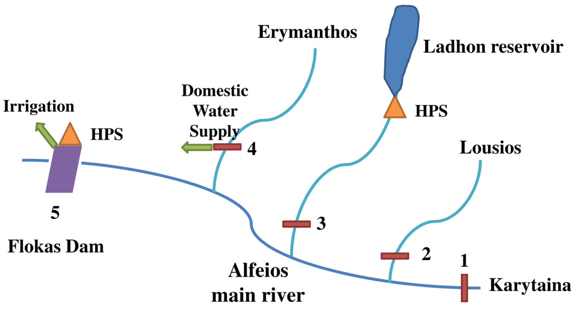
The schematization of the Alfeios river network is depicted as shown in Figure 1, including the main five water inflow locations, where historical timeseries (rain, temperature and river discharge) are available and the main water users as described above.

Table 1. Upper- (THydroLadhon⁺) and lower- (THydroLadhon⁻) bounds of optimized target for hydropower production at HPS at Ladhon.

Bounds of Optimized Target	Target Limits for Hydropower Production at Ladhon HPS (MWh)
	January	February	March	April	May	June	July	August	September	October	November	December	Annual
THydroLadhon−	11,857	12,553	11,810	11,046	11,081	8965	9077	7613	5925	7387	9427	8540	115,282
THydroLadhon+	37,353	38,947	48,311	35,391	23,237	15,868	15,598	14,233	13,642	17,062	17,971	24,276	301,890

Table 1. Upper- (THydroLadhon⁺) and lower- (THydroLadhon⁻) bounds of optimized target for hydropower production at HPS at Ladhon.

Bounds of Optimized Target	Target Limits for Hydropower Production at Ladhon HPS (MWh)
	January	February	March	April	May	June	July	August	September	October	November	December	Annual
THydroLadhon−	11,857	12,553	11,810	11,046	11,081	8965	9077	7613	5925	7387	9427	8540	115,282
THydroLadhon+	37,353	38,947	48,311	35,391	23,237	15,868	15,598	14,233	13,642	17,062	17,971	24,276	301,890

Table 2. Upper- and lower-water allocation targets for irrigation in EUR/m³.

Time Stages	Irrigation Water Demand (m3/s)
	Lower-Bound of Optimized Allocation Target	Upper-Bound of Optimized Allocation Target
	Tirrigation−	Tirrigation+
t = 1—January	0	0
t = 2—February	0	0
t = 3—March	0	6
t = 4—April	2.0	6
t = 5—May	5.0	6
t = 6—June	8.9	12
t = 7—July	11.5	12
t = 8—August	9.2	12
t = 9—September	2.7	6
t = 10—October	1.2	6
t = 11—November	0	0
t = 12—December	0	0
Annual (m3)	108,756,934	174,700,800

Table 2. Upper- and lower-water allocation targets for irrigation in EUR/m³.

Time Stages	Irrigation Water Demand (m3/s)
	Lower-Bound of Optimized Allocation Target	Upper-Bound of Optimized Allocation Target
	Tirrigation−	Tirrigation+
t = 1—January	0	0
t = 2—February	0	0
t = 3—March	0	6
t = 4—April	2.0	6
t = 5—May	5.0	6
t = 6—June	8.9	12
t = 7—July	11.5	12
t = 8—August	9.2	12
t = 9—September	2.7	6
t = 10—October	1.2	6
t = 11—November	0	0
t = 12—December	0	0
Annual (m3)	108,756,934	174,700,800

Table 3. Upper- (THydroFlokas⁺) and lower- (THydroFlokas⁻) bounds of optimized target for hydropower production at HPS at Flokas.

Bounds of Optimized Target	Target Limits for Hydropower Production at Flokas HPS (MWh)
	January	February	March	April	May	June	July	August	September	October	November	December	Annual
THydroFlokas−	1244	1740	2450	2045	1574	437	219	218	232	395	299	1129	11,982
THydroFlokas+	2379	2894	3435	2840	1861	773	251	255	571	1111	1397	2097	19,865

Table 3. Upper- (THydroFlokas⁺) and lower- (THydroFlokas⁻) bounds of optimized target for hydropower production at HPS at Flokas.

Bounds of Optimized Target	Target Limits for Hydropower Production at Flokas HPS (MWh)
	January	February	March	April	May	June	July	August	September	October	November	December	Annual
THydroFlokas−	1244	1740	2450	2045	1574	437	219	218	232	395	299	1129	11,982
THydroFlokas+	2379	2894	3435	2840	1861	773	251	255	571	1111	1397	2097	19,865

Figure 1. The simplified schematics of the Alfeios river basin

Figure 1. The simplified schematics of the Alfeios river basin

3.2. Optimization Problem of the Alfeios Hydrosystem

The goal of this optimization problem is to identify an optimal water allocation target with a maximized economic benefit over the planning period for the Alfeios river basin. Different water allocation targets are related not only to different policies for water resources management, but also to different economic implications (probabilistic penalty and opportunity loss). The penalty is associated with the nonproper water allocation/management, and therefore, resulting to shortages and spills for hydropower and for water shortage for irrigation. The optimization problem is structured as follows:

$$Max f^{\pm } = {\displaystyle \sum }_{i = 1}^3{\displaystyle \sum }_{t = 1}^T\widehat{N{B}_{t_l}^{\pm }}{T}_{t_i}^{\pm }- {\displaystyle \sum }_{i = 1}^3{\displaystyle \sum }_{t = 1}^T{\displaystyle \sum }_{k_1 = 1}^{K_1^t}{p}_{t{k}_1}P{E}_{ti}^{\pm }{Y}_{t{k}_{1}i}^{\pm }-{\displaystyle \sum }_{t = 1}^T{\displaystyle \sum }_{k_1 = 1}^{K_1^t}{p}_{t{k}_1}P{E}_{ti = 1}^{\pm }S{P}_{t{k}_{1}i = 1}^{\pm }$$

(17)

subject to:

Constraints of water-mass balance for the Ladhon reservoir:

$$R_{t{k}_1 }^{\pm }+S{P}_{t{k}_1 }^{\pm }= S_{t{k}_1 }^{\pm }+ Q_{t{k}_{1j=1}}^{\pm }-E_{1t }^{\pm }-S_{(t+1)k_1}^{\pm }, \forall t; k_1= 1, 2, \dots ,K_1^t$$

(18)

$$E_{1t }^{\pm } = e_{1t }^{\pm }\left(\frac{A_{t{k}_1 }^{\pm }+ A_{\left(t+1\right)k_1 }^{\pm }}{2}\right)$$

(19)

$$A_{t{k}_1 }^{\pm } = a_1 S_{t{k}_1 }^{\pm }+b_1$$

(20)

Constraints for the minimum and maximum water volume released by turbines at HPS Ladhon:

$$R_{t{k}_1 }^{\pm }\le TL{U}_1^{\pm } , \forall t; k_1 = 1,2, \dots ,K_1^t$$

(21)

$$R_{t{k}_1 }^{\pm }\ge TL{L}_1^{\pm } , \forall t; k_1 = 1,2, \dots ,K_1^t$$

(22)

Constraints of Ladhon reservoir capacity:

$$S_{t{k}_1 }^{\pm }\le RS{C}_1^{\pm }, \forall t; k_1 = 1,2, \dots ,K_1^t$$

(23)

$$S_{t{k}_1 }^{\pm }\ge RS{L}_1^{\pm }, \forall t; k_1 = 1,2, \dots ,K_1^t$$

(24)

Constraints for target of hydropower production at Ladhon:

$$T_{t i = 1 }^{\pm }- Y_{t{k}_1 i = 1}^{\pm } = H{P}_{t{k}_{1 } i = 1}^{\pm }, \forall t; k_1 = 1,2, \dots ,K_1^t$$

(25)

$$H{P}_{t{k}_{1 } i = 1 }^{\pm } = d_1 R_{t{k}_1 }^{\pm }+e_1, \forall t; k_1 = 1,2, \dots ,K_1^t$$

(26)

$$TH{P}_{k_{1 } i = 1 }^{\pm } = {\displaystyle \sum }_{t = 1}^{12}\left(H{P}_{t{k}_{1 } i = 1 }^{\pm }\right) , \forall k_1 = 1,2, \dots ,K_1^t$$

(27)

Constraints of water-mass balance for the Flokas Dam:

Water availability at Flokas dam based on the upstream water inflows:

$$Q_{t{k}_{1}5 }^{\pm } = {\displaystyle \sum }_{j = 2}^4{Q}_{t{k}_{1}j }^{\pm } c_{j }+R_{t{k}_1 }^{\pm }+S{P}_{t{k}_1}^{\pm }, \forall t; k_1 = 1,2, \dots ,K_1^t$$

(28)

Water-mass balance at Flokas Dam:

$$Q_{t{k}_{1}5 }^{\pm } = T_{t i = 3 }^{\pm }-WI{B}_{t{k}_1 }^{\pm }+WI{O}_{t{k}_1 }^{\pm }+WF{L}_{t{k}_1}^{\pm }, \forall t; k_1 = 1,2, \dots ,K_1^t$$

(29)

Water-mass balance at the small HPS at Flokas:

$$WI{O}_{t{k}_1 }^{\pm }= WV{F}_{t{k}_1 }^{\pm }+WVF{O}_{t{k}_1 }^{\pm }+, \forall t; k_1= 1, 2, \dots ,K_1^t$$

(30)

Constraints for target of hydropower production at Flokas:

$$T_{t i = 2 }^{\pm }- Y_{t{k}_1 i = 2}^{\pm } = H{P}_{t{k}_{1 } i = 2}^{\pm }, \forall t; k_1 = 1,2, \dots ,K_1^t$$

(31)

$$H{P}_{t{k}_{1 } i = 2 }^{\pm } = f_1 R_{t{k}_1 }^{\pm }+g_1, \forall t; k_1 = 1,2, \dots ,K_1^t$$

(32)

$$TH{P}_{k_{1 } i = 2 }^{\pm } = {\displaystyle \sum }_{t = 1}^{12}\left(H{P}_{t{k}_{1 } i = 2}^{\pm }\right),\forall k_1 = 1,2, \dots ,K_1^t$$

(33)

Constraints for the minimum and maximum water volume released by turbines at HPS at Flokas:

$$WV{F}_{t{k}_1 }^{\pm }\le TF{U}_1^{\pm }, \forall t; k_1 = 1,2, \dots ,K_1^t$$

(34)

$$WV{F}_{t{k}_1 }^{\pm }\ge TF{L}_1^{\pm }, \forall t; k_1 = 1,2, \dots ,K_1^t$$

(35)

Constraints for water allocation target of irrigation at Flokas:

$$Y_{t{k}_1 i = 3}^{\pm } = WI{B}_{t{k}_1}^{\pm }, \forall t; k_1 = 1,2, \dots ,K_1^t$$

(36)

Constraints of upper- and lower-bounds for allocation targets:

$$\widetilde{\widehat{T_{ti}^{min}}}\le {T_i}^{\pm } \le \widetilde{\widehat{T_{ti}^{max} , \forall t \text{and }i} }$$

(37)

Non-negative and technical constrains

$$T_{ti}^{\pm }\ge Y_{t{k}_1 i}^{\pm }, \forall t; k_1 = 1,2, \dots ,K_1^t ; i = 1\dots 3$$

(38)

where

$f^{\pm }=$ net system benefit over the planning horizon (EUR);

$t =$time period, and t = 1, 2, …, T (T = 12);

$A_{t{k}_1} =$surface area of Ladhon reservoir in period t under scenarios k₁ ($m^2$);

$a_1 =$slope coefficient from linear regression between surface area of Ladhon reservoir and storage volume;

$b_1 =$intercept coefficient from linear regression between surface area of Ladhon reservoir and storage volume;

$H{P}_{t{k}_{1 } i }^{\pm }=$monthly hydropower production for t = 1, 2, …, T; in period t under scenarios k₁ for the water user i with i = 1, 2 corresponding to Ladhon and Flokas, respectively;

$TH{P}_{k_{1 } i }^{\pm }=$annual hydropower production in period t under scenarios k₁ for the water user i with i = 1, 2 corresponding to Ladhon and Flokas, respectively;

$d_1 =$slope coefficient from linear regression between hydropower production of Ladhon reservoir and water volume released through the turbines;

$e_1 =$slope coefficient from linear regression between hydropower production of Ladhon reservoir and water volume released through the turbines;

$c_j =$area-based conversion factor multiplied with each stream discharge $Q_{t{k}_{1}j}^{\pm }$ to add the contribution of water inflows from intermittent drainage areas;

$f_1 =$slope coefficient from linear regression between hydropower production of Flokas and water volume released through the turbines;

$g_1 =$slope coefficient from linear regression between hydropower production of Flokas HPS and water volume released through the turbines;

$\widehat{T_{t_i}^{min}}$= lower-bound of the optimized target for the water user i in period t (($m^3$) for irrigation and (MWh) for hydropower;

$\widehat{T_{t_i}^{max}}$= upper-bound of the optimized target for the water user i in period t (($m^3$) for irrigation and (MWh) for hydropower);

$e_{1t }^{\pm }=$average evaporation rate for Ladhon reservoir in period t (m);

$E_{1t }^{\pm }=$evaporation loss of Ladhon reservoir in period t ($m^3$);

$K_1^t$= number of flow scenarios in period t;

$N{B}_i^{\pm }$ = net benefit per unit of water allocated for each water user i—(EUR/$m^3$) for irrigation and (EUR/$MWh)$ for hydropower;

$P{E}_i^{\pm }=$ penalty per unit of water not delivered (EUR/$m^3$) for each water user i—for irrigation and (EUR/$MWh)$ for hydropower; and $P{E}_t>N{B}_t$;

$p_{t{k}_1}$= probability of occurrence of scenario $k_1$ in period t, with $p_{t{k}_1}>0$ and ${{\displaystyle \sum }}_{k_1=1}^{K_1^t}{p}_{t{k}_1}=1$;

$Q_{t{k}_{1}j}^{\pm }=$water inflow level into stream j in period t under scenario $k_1$ ($m^3$);

i = 1, 2, 3 for the water users being hydropower production at Ladhon, hydropower production at Flokas and irrigation at Flokas;

j = 1, 2, 3, 4, 5 stream index for the river flows at Karytaina, Lousios, Ladhon, Erymanthos and Flokas;

$R_{t{k}_1 }^{\pm }=$release flow from the turbines of Ladhon reservoir in period t under scenario $k_1$ ($m^3$);

$S{P}_{t{k}_1 }^{\pm }=$spill volume over Ladhon Dam in period t under scenario $k_1$ ($m^3$);

$RS{C}_1^{\pm }$= maximum storage capacity of Ladhon reservoir ($m^3$);

$RS{L}_1^{\pm }$= minimum storage capacity of Ladhon reservoir ($m^3$);

$TL{U}_1^{\pm }=$maximum capacity of turbines at Ladhon HPS ($m^3$);

$TL{L}_1^{\pm }=$minimum capacity of turbines at Ladhon HPS ($m^3$);

$TF{U}_1^{\pm }=$maximum capacity of turbines at Flokas HPS ($m^3$);

$TF{L}_1^{\pm }=$ minimum capacity of turbines at Flokas HPS ($m^3$);

$S_{t{k}_1 }^{\pm }$= storage level in Ladhon reservoir in period t under scenario $k_1$ ($m^3$);

$T_{ti }^{\pm }$= water allocation target that is promised to the user i in period t ($m^3$);

$Y_{t{k}_{1}i}^{\pm }=$shortage level by which the water-allocation target is not met in period t under scenarios $k_1$ for the water user i, which is associated with probability of $p_{t{k}_1}$—($m^3$) for irrigation and MWh for hydropower;

$WI{B}_{t{k}_1 }^{\pm }=$irrigation shortage volume in period t under scenarios $k_1$ ($m^3$);

$WI{O}_{t{k}_1 }^{\pm }=$water volume left at Flokas after having allocated the irrigation water in period t under scenarios $k_1$ ($m^3$);

$WF{L}_{t{k}_1 }^{\pm }=$water volume flowing through the fish ladder at Flokas dam in period t under scenarios $k_1$($m^3$);

$WV{F}_{t{k}_1 }^{\pm }$= water volume flowing through the turbines at Flokas HPS in period t under scenarios $k_1$ ($m^3$);

$WVF{O}_{t{k}_1 }^{\pm }=$spill volume at Flokas dam in period t under scenarios $k_1$ ($m^3$);

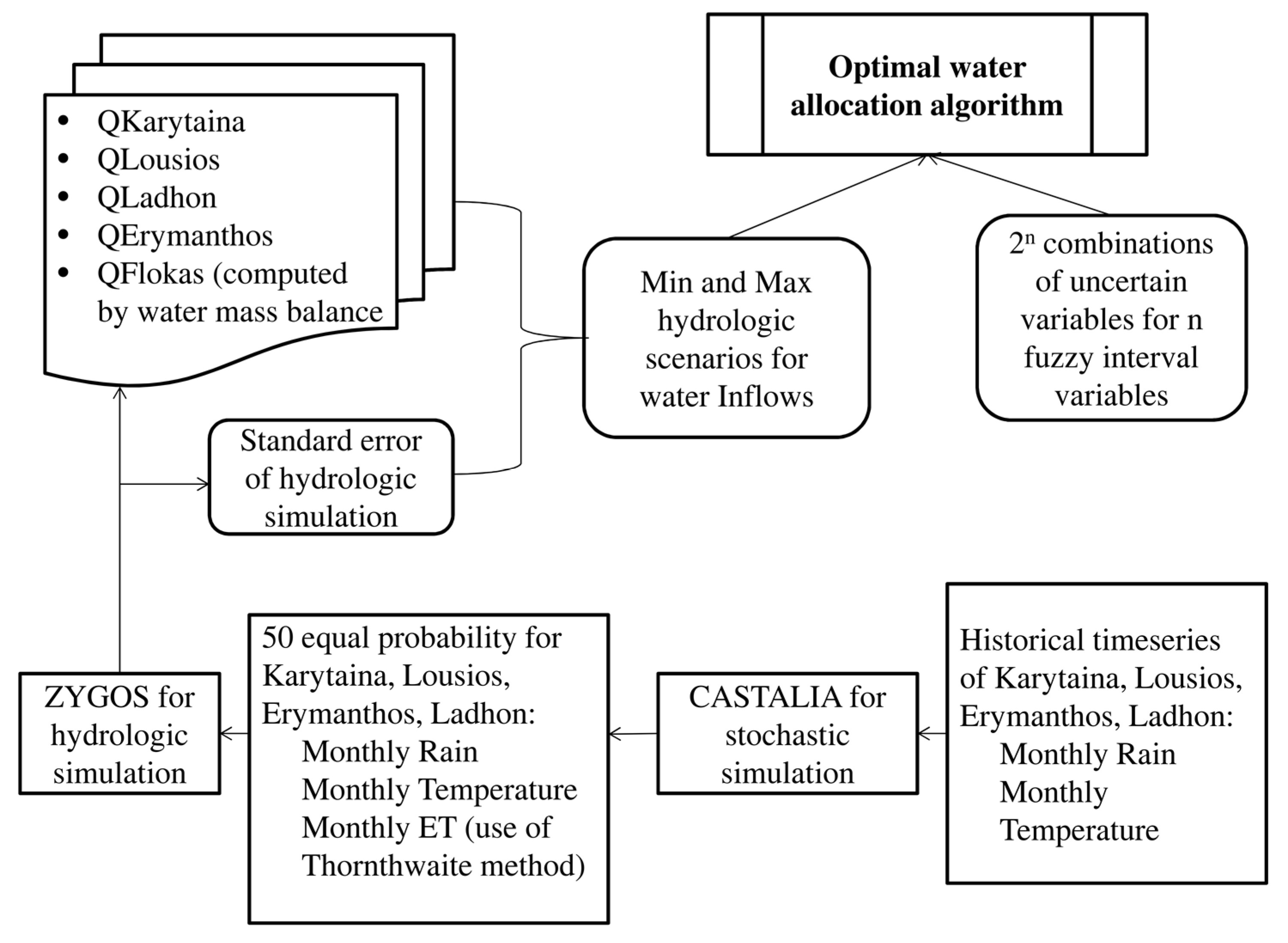
CASTALIA model is applied for the simultaneous stochastic generation of fifty equal-probability scenarios for the hydrologic variables of rain and temperature at the four considered subcatchments (Karytaina, Lousios, Ladhon and Erymanthos) having a time length of ten years (since the future WADI water and agriculture scenarios are projected ten years after the baseline scenario) and monthly time step. The stochastically simulated rain and temperature timeseries are introduced into the calibrated simple lumped conceptual river basin model ZYGOS [58,59] for the four subcatchments in order to compute the mean monthly discharges for this ten years period. The uncertainty from the hydrologic model structure and the parametrization is taken into account through the computation of the standard error between the measured and the simulated water discharge timeseries. Based on this standard error, upper-bound water inflows timeseries for all the hydrologic scenarios (which are used in the f⁺ model), and lower-bound (which are used in the f⁻ model) are created. The steps of this process and the software programs used are presented schematically in the form of a flow chart in Figure 2. The last year of each of the fifty stochastic monthly discharge scenarios (since the future scenarios refer to ten years after the baseline) serves as input inflows into the optimization model for the optimal water allocation of Alfeios river basin. The monthly discharge at Flokas Dam, which is of interest for the optimization process, since at this position the available water is diverted to the irrigation canal, is computed as the sum of the four subcatchments as described in [38].

In the optimization problem, there are some nonlinear equations, such as the relationship between water flowing through the turbines and the hydropower energy produced. In order to introduce them into the linear programming algorithm their linear regression equations are considered. The uncertainty resulting from this simplification has not been considered in the process, but it is worth mentioning that in all cases the R² takes values ≥ 0.9.

Figure 2. Methodological framework for optimal water allocation of Alfeios river basin.

Figure 2. Methodological framework for optimal water allocation of Alfeios river basin.

The uncertain variables in this case are firstly, the coefficients of the objective function including (a) the unit benefits and penalties from hydropower production of Ladhon (EUR/MWh); (b) the unit benefits and penalties from the hydropower of Flokas (EUR/MWh); and (c) the unit benefits and penalties from Flokas irrigation (EUR/m³), and secondly, the initial water level of Ladhon reservoir at stage zero (m³) which is expressed as deterministic-boundary interval (12,362,644.01, 26,783,729.12). A detailed analysis of the estimation of the prementioned unit benefits and penalties is provided in [38]. Briefly, based on the estimations of the Chief Engineer at Ladhon hydropower station, the upper- and lower- fuzzy-boundary intervals for the unit benefit and penalty of Ladhon are defined as given in Table 4. The shadow penalty for the hydropower production at Ladhon is composed of two parts: (a) the penalty due to hydropower shortage in comparison to the hydropower production target and (b) the penalty for the water spilled from the Ladhon Dam (if any) and is not available for hydropower production, which intends to express the opportunity loss of hydropower energy production. Based on the monthly selling price data of Flokas HPS, its unit benefit is approximated as a single deterministic interval (and not as a fuzzy-boundary interval) as presented in Table 4. The unit shadow penalty is approximated as a single deterministic interval and is taken equal to the upper-bound solution of the unit penalty of Flokas HPS, as shown in Table 4. The unit benefit for water allocated to irrigation is interpreted as the probable net income from agricultural production of the Flokas crop pattern, taking into account the brutto farmer, the cost of production, the cost of the irrigation canal (associated to the water charge to the farmers from the general irrigation organization) and the organizational structure of local irrigation organizations (the charges of the local irrigation organizations). In Table 5, the lower- and upper- fuzzy-boundaries of the unit benefit of water allocated to the Flokas irrigation scheme is provided for the baseline scenario and the WADI future scenarios. Finally, the unit penalty from the irrigation water deficits is based on the crop yield reduction and the corresponding net farmer income loss. In Table 6 the lower- and upper- fuzzy-boundaries of the unit penalties for irrigation water deficits of the Flokas irrigation scheme is provided for the baseline scenario and the WADI future scenarios (where as presented in Section 4 the World agricultural markets scenario is denoted as Future Scenario 1 (FS1), the Global agricultural sustainability scenario as Future Scenario 2 (FS2), the Provincial agriculture scenario as (Future Scenario 3-FS3) and the Local community agriculture as (Future Scenario 4-FS4).

Table 4. Lower- and upper- fuzzy-boundary intervals for the unit benefit and unit penalty for hydropower production EUR/MWh at Ladhon and at Flokas.

Variables	NBHP Ladhon	NBHP Flokas	CHP Ladhon	CHP Flokas
	EUR/MWh	EUR/MWh	EUR/MWh	EUR/MWh
Lower-Bound—Minimum	40	87.5	120	140
Lower-Bound—Maximum	55	–	130	150
Upper-Bound—Minimum	60	80	140	140
Upper-Bound—Maximum	75	–	150	150

Table 4. Lower- and upper- fuzzy-boundary intervals for the unit benefit and unit penalty for hydropower production EUR/MWh at Ladhon and at Flokas.

Variables	NBHP Ladhon	NBHP Flokas	CHP Ladhon	CHP Flokas
	EUR/MWh	EUR/MWh	EUR/MWh	EUR/MWh
Lower-Bound—Minimum	40	87.5	120	140
Lower-Bound—Maximum	55	–	130	150
Upper-Bound—Minimum	60	80	140	140
Upper-Bound—Maximum	75	–	150	150

Table 5. Lower- and upper- fuzzy-boundary intervals for the unit benefit from irrigation for the baseline and the WADI future scenarios for Flokas irrigation scheme EUR/m³.

Fuzzy-Boundary Intervals		NBIrrigationFlokas EUR/m3
		Baseline	FS 1	FS 2	FS 3	FS 4
Upper-Bound	Min	0.166	0.127	0.189	0.191	0.221
	Max	0.175	0.136	0.265	0.276	0.294
Lower-Bound	Min	0.187	0.190	0.266	0.277	0.295
	Max	0.205	0.234	0.269	0.314	0.431

FS1: Future Scenario 1; FS2: Future Scenario 2; FS3: Future Scenario 3; FS4: Future Scenario 4.

Table 5. Lower- and upper- fuzzy-boundary intervals for the unit benefit from irrigation for the baseline and the WADI future scenarios for Flokas irrigation scheme EUR/m³.

Fuzzy-Boundary Intervals		NBIrrigationFlokas EUR/m3
		Baseline	FS 1	FS 2	FS 3	FS 4
Upper-Bound	Min	0.166	0.127	0.189	0.191	0.221
	Max	0.175	0.136	0.265	0.276	0.294
Lower-Bound	Min	0.187	0.190	0.266	0.277	0.295
	Max	0.205	0.234	0.269	0.314	0.431

FS1: Future Scenario 1; FS2: Future Scenario 2; FS3: Future Scenario 3; FS4: Future Scenario 4.

Table 6. Lower- and upper- fuzzy-boundary intervals for the unit penalties for water deficits to irrigation EUR/m³ for the baseline and the future scenarios.

Fuzzy-Boundary Intervals		PEIrrigationFlokas EUR/m3
		Baseline	FS 1	FS 2	FS 3	FS 4
Upper-Bound	Min	0.989	0.748	1.052	1.035	1.043
	Max	1.051	1.159	1.075	1.073	1.070
Lower-Bound	Min	1.715	3.361	1.537	1.552	2.184
	Max	1.812	3.410	1.891	1.871	2.279

FS1: Future Scenario 1; FS2: Future Scenario 2; FS3: Future Scenario 3; FS4: Future Scenario 4.

Table 6. Lower- and upper- fuzzy-boundary intervals for the unit penalties for water deficits to irrigation EUR/m³ for the baseline and the future scenarios.

Fuzzy-Boundary Intervals		PEIrrigationFlokas EUR/m3
		Baseline	FS 1	FS 2	FS 3	FS 4
Upper-Bound	Min	0.989	0.748	1.052	1.035	1.043
	Max	1.051	1.159	1.075	1.073	1.070
Lower-Bound	Min	1.715	3.361	1.537	1.552	2.184
	Max	1.812	3.410	1.891	1.871	2.279

FS1: Future Scenario 1; FS2: Future Scenario 2; FS3: Future Scenario 3; FS4: Future Scenario 4.

4. WADI Water and Agriculture Future Scenarios

The Sustainability of European Irrigated Agriculture under Water Framework Directive and Agenda 2000 project (WADI) focuses on changes in EU agricultural and water policy as they affect the economic, social and environmental performance of irrigation in the partner countries [39]. Its aim was to investigate the impacts of policy change on the irrigation sector in Spain, Greece, Italy and the UK with a particular focus on Water Framework Directive (WFD) and the reform of Common Agricultural Policy (CAP). The agricultural policy regime in place in 2001, as determined by CAP at that time is taken as baseline scenario. This 2001 baseline year is used to provide a relative reference point for the definition of future scenarios. This scenario is extrapolated to 10 years after the reference year (thus from 2001 to 2010) based on predictions (rather than possibilities) of agricultural markets and prices from EU, the Organization for Economic Co-operation and Development (OCDE) and other sources. The estimates of the main parameters (Table 7), determined for each future scenario, are used within this paper as inputs in the developed optimal water allocation model based on [2] under uncertain and vague water system conditions in order to enable the assessment of the impact of the EU agricultural and water policy changes on the hydrosystem’s benefits of the baseline scenario.

Table 7. Analysis of the Foresight scenarios based on the regional analysis in [39,40]—expressed as a percentage of the baseline year at constant values.

Crop Prices	Baseline	World Agricultural Markets		Global Agricultural Sustainability		Provincial Agriculture		Local Community Agriculture
Crops selling prices perceived by the farmers	–	Min	Max	Min	Max	Min	Max	Min	Max
Maize	100	85	95	95	105	100	110	100	110
Maize area subsidy	100	0	–	75	85	90	100	85	95
Set aside quota	100	0	–	95	–	100	–	105	–
Tomato	100	85	95	110	120	100	110	120	130
Potato	100	85	95	95	105	105	115	120	130
Watermelons	100	85	95	95	105	105	115	120	130
Cotton	100	80	90	90	100	85	95	110	120
Cotton subsidy	100	0	–	85	–	90	–	105	–
Olive Trees	100	80	90	85	95	90	100	100	110
Olive trees area subsidy	100	0	–	95	–	95	–	105	–
Alfalfa	100	80	90	90	100	100	110	110	120
Citrus	100	85	95	95	105	100	110	120	130
Input prices	–	Min	Max	Min	Max	Min	Max	Min	Max
Fertilizers	100	85	100	140	150	100	110	150	160
Pesticides	100	110	120	100	105	105	115	95	100
Energy	100	85	95	120	130	100	110	130	140
Seeds	100	100	110	110	120	120	130	130	140
Machinery	100	100	115	115	135	100	115	120	140
Contractor services	100	130	135	120	130	130	140	110	120
Water prices	100	100	110	115	130	100	110	120	140
Irrigation infrastructure	100	100	110	120	130	115	125	130	150
Labour	100	90	100	100	110	95	105	110	120
Land	100	110	120	110	125	100	110	85	95
Other inputs	100	85	95	125	135	85	95	130	140
Crop yield changes due to technology	100	110	120	100	115	100	105	85	105
Restriction on chemical use	100	130	140	120	130	110	120	100	110

Table 7. Analysis of the Foresight scenarios based on the regional analysis in [39,40]—expressed as a percentage of the baseline year at constant values.

Crop Prices	Baseline	World Agricultural Markets		Global Agricultural Sustainability		Provincial Agriculture		Local Community Agriculture
Crops selling prices perceived by the farmers	–	Min	Max	Min	Max	Min	Max	Min	Max
Maize	100	85	95	95	105	100	110	100	110
Maize area subsidy	100	0	–	75	85	90	100	85	95
Set aside quota	100	0	–	95	–	100	–	105	–
Tomato	100	85	95	110	120	100	110	120	130
Potato	100	85	95	95	105	105	115	120	130
Watermelons	100	85	95	95	105	105	115	120	130
Cotton	100	80	90	90	100	85	95	110	120
Cotton subsidy	100	0	–	85	–	90	–	105	–
Olive Trees	100	80	90	85	95	90	100	100	110
Olive trees area subsidy	100	0	–	95	–	95	–	105	–
Alfalfa	100	80	90	90	100	100	110	110	120
Citrus	100	85	95	95	105	100	110	120	130
Input prices	–	Min	Max	Min	Max	Min	Max	Min	Max
Fertilizers	100	85	100	140	150	100	110	150	160
Pesticides	100	110	120	100	105	105	115	95	100
Energy	100	85	95	120	130	100	110	130	140
Seeds	100	100	110	110	120	120	130	130	140
Machinery	100	100	115	115	135	100	115	120	140
Contractor services	100	130	135	120	130	130	140	110	120
Water prices	100	100	110	115	130	100	110	120	140
Irrigation infrastructure	100	100	110	120	130	115	125	130	150
Labour	100	90	100	100	110	95	105	110	120
Land	100	110	120	110	125	100	110	85	95
Other inputs	100	85	95	125	135	85	95	130	140
Crop yield changes due to technology	100	110	120	100	115	100	105	85	105
Restriction on chemical use	100	130	140	120	130	110	120	100	110

To provide a better understanding of the content and the philosophy of each future scenario, the four WADI agricultural and water scenarios are briefly described based on [39,40]. World Markets scenario is related to private consumption and a highly developed and integrated world trading system. Global Sustainability scenario poses emphasis on social and ecological values associated with global institutions and trading systems. In comparison to the first scenario, slow but more equally distributed growth is considered. Active public policy and international co-operation within the European Union and at a global level are central. Provincial Enterprise scenario emphasizes private consumption within national and regional level to depict local priorities and interests. The dominance of market values is noticed within the national/regional boundaries. Provincial agricultural markets scenario is also characterized by protectionist regimes similar to that under pre-reform Common Agricultural Policy. People aspire to personal independence and material wealth within a nationally rooted cultural identity. Local Stewardship scenario is focused on strong local or regional governments with emphasis on social values, self-reliance, self-sufficiency, and conservation of natural resources and the environment. Local community agriculture scenario emphasizes sustainability at a local level. In the following tables the World agricultural markets scenario is denoted as Future Scenario 1 (FS1), the Global agricultural sustainability scenario as Future Scenario 2 (FS2), the Provincial agriculture scenario as (Future Scenario 3-FS3) and the Local community agriculture as (Future Scenario 4-FS4).

5. Results

In the proposed methodology, two types of solution methods, an optimistic (1st solution method, also called as risk-prone by [2]) and a pessimistic (2nd solution method, also called as risk-adverse by [2]), have been incorporated in order to compute the optimized water allocation targets under uncertain system conditions. The term of “risk”, used to characterize these two different solution approaches, does not imply the measuring of risk with its strict mathematical definition, but the willingness of the decision makers to take the risk or not of economic penalty or of opportunity loss associated with their attitude concerning the uncertainties’ values of the optimization problem as described below. According to [2], in general, the first solution method could identify the highest system benefit, but may be, however, associated with higher risk since it is based on an optimistic anticipation for the system components. The second solution method could assist to compute a narrower interval for the system benefit with a lower risk, since it is based on a conservative anticipation for system components and constraints, but the system might lose the opportunity of achieving the highest benefit value.

The solution in terms of the objective function value (meaning the total net benefit) results to a fuzzy-boundary interval for each α-cut level and each solution method [($\underset{\_}{f_{opt}^{-}}$), ($\underset{\_}{f_{opt}^{+}}$), ($\overline{f_{opt}^{-}}$, $\overline{f_{opt}^{+}}$)]^α composed of four options of maximized system benefits in combination with minimized probabilistic penalties corresponding to different system conditions. These four options for each solution method correspond to lower-min $\underset{\_}{f_{opt}^{-}}$ (and in tables and figures written as min (f⁻)), lower-max $\underset{\_}{f_{opt}^{+}}$ (and in tables and figures written as max (f⁻)), upper-min $\overline{f_{opt}^{-}}$ (and in tables and figures written as min (f⁺)), upper-max $\overline{f_{opt}^{+}}$ (and in tables and figures written as max (f⁺)). These results (four prementioned options), however, do not necessarily construct a set of stable intervals [2].

For the Alfeios river basin considering five uncertain variables (as analyzed in Section 3.2) with fuzzy-boundary intervals and two uncertain variables with deterministic-boundary intervals (Table 4, Table 5 and Table 6), 2⁵ = 32 possible combinations of the uncertain variable values/runs of the algorithm for each WADI future scenario (32 × 5 = 160 runs for all examined scenarios in total) has been undertaken based on the FBISP algorithm as proposed by [2].

For each examined case/run (1) the optimized water allocation target for each time stage (the twelve months of the examined year), as well as for total annual (as the summation of the values of the twelve time stages); (2) the probabilistic shortages and allocations for each one of the fifty hydrologic scenarios and for each of the three water users for each time stage (the twelve months of the examined year), as well as for the total annual (as the summation of the values of the twelve time stages) and (3) the total benefits and the benefits and penalties for each of the three water users are derived. The analysis of these results is divided in two parts: (a) the analysis for the results of the baseline scenario, enabling the understanding of the optimization technique used and (b) the comparison of the results between the baseline and the future WADI water and agriculture scenarios in order to assess the effect of the EU water and agricultural policy changes in the system benefits and penalties on the baseline scenario.

5.1. Results Analysis for the Baseline Scenario

The total annual maximized net benefits of the Alfeios hydrosystem for the two solution methods are presented in Table 8. The first solution method estimates a wider range for the objective function value (meaning the total net benefits) equal to [(96,192,950, 102,180,847), (127,801,604, 135,950,230)] in EUR, but at the same time it embodies a higher uncertainty or risk. The second solution process, on the other hand, results to a narrower interval for the objective function value method [(104,523,859, 109,324,450), (128,786,579, 134,978,247)], being related to a more conservative view of the uncertainties of the hydrosystem and to the incapability to derive higher benefits under favorable conditions. The interval solution can be easily interpreted for generating decision alternatives, where upper-bound (first solution method) system benefits is associated with more advantageous conditions (e.g., associated with upper-bound inflows, upper-bound benefit coefficients, lower-bound cost coefficients, upper-bound reservoirs capacities, lower-bound reserved storage requirements) while the lower-bound (second solution method) one corresponds to the demanding conditions [1].

Table 8. Total annual net benefit (EUR) for all water uses.

WADI Scenarios	Total Annual Net Benefit (EUR)
	1st Solution Method				2nd Solution Method
	Min (f−)	Max (f−)	Min (f+)	Max (f+)	Min (f−)	Max (f−)	Min (f+)	Max (f+)
Baseline	96,192,950	102,180,847	127,801,604	135,950,230	104,523,859	109,324,450	128,786,579	134,978,247
FS1	76,667,389	81,865,504	113,991,044	126,002,601	84,858,261	89,043,374	114,966,693	125,209,412
FS2	127,853,717	147,770,816	179,855,724	187,230,205	140,082,873	157,717,364	181,108,510	185,941,332
FS3	100,450,661	119,991,812	143,479,720	154,964,308	108,428,316	126,072,379	144,472,397	154,016,575
FS4	139,941,260	159,235,851	194,409,861	225,532,763	152,798,364	169,543,642	195,726,034	224,148,365

FS1: Future Scenario 1; FS2: Future Scenario 2; FS3: Future Scenario 3; FS4: Future Scenario 4.

Table 8. Total annual net benefit (EUR) for all water uses.

WADI Scenarios	Total Annual Net Benefit (EUR)
	1st Solution Method				2nd Solution Method
	Min (f−)	Max (f−)	Min (f+)	Max (f+)	Min (f−)	Max (f−)	Min (f+)	Max (f+)
Baseline	96,192,950	102,180,847	127,801,604	135,950,230	104,523,859	109,324,450	128,786,579	134,978,247
FS1	76,667,389	81,865,504	113,991,044	126,002,601	84,858,261	89,043,374	114,966,693	125,209,412
FS2	127,853,717	147,770,816	179,855,724	187,230,205	140,082,873	157,717,364	181,108,510	185,941,332
FS3	100,450,661	119,991,812	143,479,720	154,964,308	108,428,316	126,072,379	144,472,397	154,016,575
FS4	139,941,260	159,235,851	194,409,861	225,532,763	152,798,364	169,543,642	195,726,034	224,148,365

FS1: Future Scenario 1; FS2: Future Scenario 2; FS3: Future Scenario 3; FS4: Future Scenario 4.

The total annual benefits and penalties for the irrigation at Flokas, for the hydropower production at Ladhon HPS and for the hydropower production at Flokas HPS are given in Table 9, Table 10 and Table 11. From these tables, it is shown that for the second (pessimistic) solution method the benefits are lower but also the penalties are lower in comparison to the corresponding results from the first (optimistic) solution method.

Table 9. Total annual benefit and penalties (EUR) for irrigation at Flokas.

WADI Scenarios	Total Annual Benefits (EUR)
	1st Solution Method				2nd Solution Method
	Min (f−)	Max (f−)	Min (f+)	Max (f+)	Min (f−)	Max (f−)	Min (f+)	Max (f+)
Baseline	29,064,003	30,643,655	32,706,273	35,881,125	26,641,243	28,170,265	32,706,273	35,881,125
FS1	20,626,258	22,151,608	33,275,869	40,903,212	19,075,077	20,587,187	33,275,869	40,903,212
FS2	32,942,354	46,373,935	46,548,636	46,988,116	30,191,272	44,417,804	46,548,636	46,988,116
FS3	33,406,833	48,219,300	48,394,001	54,915,529	30,710,414	46,185,328	48,394,001	54,915,529
FS4	38,614,195	51,370,227	51,544,928	75,236,645	35,390,899	47,823,846	51,544,928	75,236,645
WADI Scenarios	Total Annual Penalties (EUR)
Baseline	2,470,856	2,611,203	432,349	459,697	2,257,577	2,385,810	118,146	581,477
FS1	3,245,851	3,292,577	326,846	506,598	2,452,467	2,586,774	54,110	382,445
FS2	2,214,386	2,724,846	459,945	469,950	2,298,278	3,527,484	125,687	594,446
FS3	2,235,536	2,696,322	452,675	469,307	2,485,131	3,675,421	123,700	593,634
FS4	3,146,448	3,283,159	456,063	467,608	2,874,068	3,650,108	124,626	591,484

FS1: Future Scenario 1; FS2: Future Scenario 2; FS3: Future Scenario 3; FS4: Future Scenario 4.

Table 9. Total annual benefit and penalties (EUR) for irrigation at Flokas.

WADI Scenarios	Total Annual Benefits (EUR)
	1st Solution Method				2nd Solution Method
	Min (f−)	Max (f−)	Min (f+)	Max (f+)	Min (f−)	Max (f−)	Min (f+)	Max (f+)
Baseline	29,064,003	30,643,655	32,706,273	35,881,125	26,641,243	28,170,265	32,706,273	35,881,125
FS1	20,626,258	22,151,608	33,275,869	40,903,212	19,075,077	20,587,187	33,275,869	40,903,212
FS2	32,942,354	46,373,935	46,548,636	46,988,116	30,191,272	44,417,804	46,548,636	46,988,116
FS3	33,406,833	48,219,300	48,394,001	54,915,529	30,710,414	46,185,328	48,394,001	54,915,529
FS4	38,614,195	51,370,227	51,544,928	75,236,645	35,390,899	47,823,846	51,544,928	75,236,645
WADI Scenarios	Total Annual Penalties (EUR)
Baseline	2,470,856	2,611,203	432,349	459,697	2,257,577	2,385,810	118,146	581,477
FS1	3,245,851	3,292,577	326,846	506,598	2,452,467	2,586,774	54,110	382,445
FS2	2,214,386	2,724,846	459,945	469,950	2,298,278	3,527,484	125,687	594,446
FS3	2,235,536	2,696,322	452,675	469,307	2,485,131	3,675,421	123,700	593,634
FS4	3,146,448	3,283,159	456,063	467,608	2,874,068	3,650,108	124,626	591,484

FS1: Future Scenario 1; FS2: Future Scenario 2; FS3: Future Scenario 3; FS4: Future Scenario 4.

Table 10. Total annual benefit and penalties (EUR) for hydropower production at Ladhon HPS.

WADI Scenarios	Total Annual Benefits (EUR)
	1st Solution Method				2nd Solution Method
	Min (f−)	Max (f−)	Min (f+)	Max (f+)	Min (f−)	Max (f−)	Min (f+)	Max (f+)
Baseline	11,027,398	15,924,814	16,711,593	21,878,560	7,346,406	10,657,147	11,202,510	14,950,226
FS1	9,373,289	13,536,092	14,204,854	18,596,776	6,161,067	9,059,977	9,513,407	12,692,143
FS2	15,438,358	22,294,739	23,396,230	30,629,985	10,261,288	14,920,853	15,683,515	20,954,784
FS3	11,027,398	15,924,814	16,711,593	21,878,560	7,346,676	10,657,666	11,203,456	14,967,703
FS4	16,541,098	23,887,221	25,067,389	32,817,841	11,000,389	15,986,499	16,803,766	22,427,814
WADI Scenarios	Total Annual Penalties (EUR)
Baseline	18,854,936	20,501,510	7,598,174	8,375,765	4,805,658	5,564,719	1,655,029	2,279,614
FS1	16,003,268	17,401,182	6,458,448	7,119,400	4,065,699	4,711,214	1,401,002	1,930,522
FS2	26,396,911	28,702,114	10,637,443	11,726,070	6,727,922	7,830,586	2,341,889	3,210,311
FS3	18,854,936	20,501,510	7,598,174	8,375,765	4,807,341	5,593,869	1,655,633	2,293,079
FS4	28,282,404	30,752,265	11,397,261	12,563,647	7,208,488	8,354,489	2,689,422	3,425,385

FS1: Future Scenario 1; FS2: Future Scenario 2; FS3: Future Scenario 3; FS4: Future Scenario 4.

Table 10. Total annual benefit and penalties (EUR) for hydropower production at Ladhon HPS.

WADI Scenarios	Total Annual Benefits (EUR)
	1st Solution Method				2nd Solution Method
	Min (f−)	Max (f−)	Min (f+)	Max (f+)	Min (f−)	Max (f−)	Min (f+)	Max (f+)
Baseline	11,027,398	15,924,814	16,711,593	21,878,560	7,346,406	10,657,147	11,202,510	14,950,226
FS1	9,373,289	13,536,092	14,204,854	18,596,776	6,161,067	9,059,977	9,513,407	12,692,143
FS2	15,438,358	22,294,739	23,396,230	30,629,985	10,261,288	14,920,853	15,683,515	20,954,784
FS3	11,027,398	15,924,814	16,711,593	21,878,560	7,346,676	10,657,666	11,203,456	14,967,703
FS4	16,541,098	23,887,221	25,067,389	32,817,841	11,000,389	15,986,499	16,803,766	22,427,814
WADI Scenarios	Total Annual Penalties (EUR)
Baseline	18,854,936	20,501,510	7,598,174	8,375,765	4,805,658	5,564,719	1,655,029	2,279,614
FS1	16,003,268	17,401,182	6,458,448	7,119,400	4,065,699	4,711,214	1,401,002	1,930,522
FS2	26,396,911	28,702,114	10,637,443	11,726,070	6,727,922	7,830,586	2,341,889	3,210,311
FS3	18,854,936	20,501,510	7,598,174	8,375,765	4,807,341	5,593,869	1,655,633	2,293,079
FS4	28,282,404	30,752,265	11,397,261	12,563,647	7,208,488	8,354,489	2,689,422	3,425,385

FS1: Future Scenario 1; FS2: Future Scenario 2; FS3: Future Scenario 3; FS4: Future Scenario 4.

In Table 12 the optimized targets of annual water volume for irrigation (m³) and of annual hydropower production at HPS Ladhon and Flokas (MWh) for the two different solution processes of the model are presented for the baseline scenario and the four future WADI scenarios. For the irrigation at Flokas the range of the optimized target of the annual water volume for the upper-bound model (f⁺) is the same for both solution methods and is equal to its maximum possible value of 174,700,800 m³. For the lower-bound model (f⁻) higher maximum allocation targets are computed by the first solution method (160,079,569, 174,700,800) with much wider ranges between the minimum and the maximum value (14,621,231 m³) compared to the ones from the second solution method (160,574,718, 160,599,895) with corresponding range (25,177 m³). By comparing the corresponding results of the FBISP method in this paper with the ITSP as presented in [38], it is worth noticing that the monthly optimized water allocation target values for irrigation at Flokas are equal to the maximum possible allocation for the upper- and the lower-bound solution of the ITSP. This shows that the incorporation of the fuzzy nature of the uncertainties in the FBISP results in lower optimized water allocation target values for the lower-bound (second solution method) solution, reflecting a more analytic and fine approximation of the effect of the uncertainties on the minimum and maximum values of the boundaries of the results.

Table 11. Total annual benefit and penalties (EUR) for hydropower production at Flokas HPS.

WADI scenarios	Total Annual Benefits (EUR)
	1st Solution Method				2nd Solution Method
	Min (f−)	Max (f−)	Min (f+)	Max (f+)	Min (f−)	Max (f−)	Min (f+)	Max (f+)
Baseline	79,312,739	79,312,739	86,996,160	86,996,160	79,312,739	79,312,739	86,996,160	86,996,160
FS1	67,415,828	67,415,828	73,946,736	73,946,736	67,415,828	67,415,828	73,946,736	73,946,736
FS2	111,037,834	111,037,834	121,794,624	121,794,624	111,037,834	111,037,834	121,794,624	121,794,624
FS3	79,312,739	79,312,739	86,996,160	86,996,160	79,312,739	79,312,739	86,996,160	86,996,160
FS4	118,969,108	118,969,108	130,494,240	130,494,240	118,969,108	118,969,108	130,494,240	130,494,240
WADI scenarios	Total Annual Penalties (EUR)
Baseline	1,294,736	1,295,664	235,104	244,521	1,279,939	1,284,407	196,202	199,798
FS1	1,071,046	1,071,835	199,839	207,843	1,064,610	1,070,039	168,108	172,620
FS2	1,812,630	1,813,930	329,146	342,330	1,791,914	1,821,487	272,398	279,717
FS3	1,294,736	1,295,664	235,104	244,521	1,281,003	1,301,062	194,570	199,372
FS4	1,942,104	1,943,496	352,657	366,782	1,919,908	1,934,281	292,242	299,697

FS1: Future Scenario 1; FS2: Future Scenario 2; FS3: Future Scenario 3; FS4: Future Scenario 4.

Table 11. Total annual benefit and penalties (EUR) for hydropower production at Flokas HPS.

WADI scenarios	Total Annual Benefits (EUR)
	1st Solution Method				2nd Solution Method
	Min (f−)	Max (f−)	Min (f+)	Max (f+)	Min (f−)	Max (f−)	Min (f+)	Max (f+)
Baseline	79,312,739	79,312,739	86,996,160	86,996,160	79,312,739	79,312,739	86,996,160	86,996,160
FS1	67,415,828	67,415,828	73,946,736	73,946,736	67,415,828	67,415,828	73,946,736	73,946,736
FS2	111,037,834	111,037,834	121,794,624	121,794,624	111,037,834	111,037,834	121,794,624	121,794,624
FS3	79,312,739	79,312,739	86,996,160	86,996,160	79,312,739	79,312,739	86,996,160	86,996,160
FS4	118,969,108	118,969,108	130,494,240	130,494,240	118,969,108	118,969,108	130,494,240	130,494,240
WADI scenarios	Total Annual Penalties (EUR)
Baseline	1,294,736	1,295,664	235,104	244,521	1,279,939	1,284,407	196,202	199,798
FS1	1,071,046	1,071,835	199,839	207,843	1,064,610	1,070,039	168,108	172,620
FS2	1,812,630	1,813,930	329,146	342,330	1,791,914	1,821,487	272,398	279,717
FS3	1,294,736	1,295,664	235,104	244,521	1,281,003	1,301,062	194,570	199,372
FS4	1,942,104	1,943,496	352,657	366,782	1,919,908	1,934,281	292,242	299,697

FS1: Future Scenario 1; FS2: Future Scenario 2; FS3: Future Scenario 3; FS4: Future Scenario 4.

Table 12. Optimized target for total annual water volumes for irrigation (m³).

Irrigation (m3)	Optimized Target for Total Annual Water Volumes for Irrigation (m3)
	1st Solution Method			2nd Solution Method
	Min (f−)	Max (f−)	Min (f+)	Max (f+)	Min (f−)	Max (f−)	Min (f+)	Max (f+)
Baseline	160,079,569	174,700,800	174,700,800	174,700,800	160,574,718	160,599,895	174,700,800	174,700,800
FS1	150,527,097	162,767,927	174,700,800	174,700,800	151,272,706	151,272,706	174,700,800	174,700,800
FS2	160,079,569	174,700,800	174,700,800	174,700,800	167,331,623	167,331,623	174,700,800	174,700,800
FS3	160,541,634	174,700,800	174,700,800	174,700,800	167,331,623	167,331,623	174,700,800	174,700,800
FS4	160,079,569	174,700,800	174,700,800	174,700,800	162,606,691	162,640,203	174,700,800	174,700,800

FS1: Future Scenario 1; FS2: Future Scenario 2; FS3: Future Scenario 3; FS4: Future Scenario 4.

Table 12. Optimized target for total annual water volumes for irrigation (m³).

Irrigation (m3)	Optimized Target for Total Annual Water Volumes for Irrigation (m3)
	1st Solution Method			2nd Solution Method
	Min (f−)	Max (f−)	Min (f+)	Max (f+)	Min (f−)	Max (f−)	Min (f+)	Max (f+)
Baseline	160,079,569	174,700,800	174,700,800	174,700,800	160,574,718	160,599,895	174,700,800	174,700,800
FS1	150,527,097	162,767,927	174,700,800	174,700,800	151,272,706	151,272,706	174,700,800	174,700,800
FS2	160,079,569	174,700,800	174,700,800	174,700,800	167,331,623	167,331,623	174,700,800	174,700,800
FS3	160,541,634	174,700,800	174,700,800	174,700,800	167,331,623	167,331,623	174,700,800	174,700,800
FS4	160,079,569	174,700,800	174,700,800	174,700,800	162,606,691	162,640,203	174,700,800	174,700,800

FS1: Future Scenario 1; FS2: Future Scenario 2; FS3: Future Scenario 3; FS4: Future Scenario 4.

Generally, the shortage of a water user (irrigation or hydropower production) is the result of the nonsatisfaction of the predefined target for the examined water use and is expressed as the difference between target value and available water. Therefore, the water allocation is given by the difference between the target value and the probabilistic shortage. The results for the annual shortage (Table 13) and the annual allocation (Table 14) for irrigation, as computed by the optimization algorithm from the two solution methods and for the fifty hydrologic equal-probability scenarios are presented. As shown in Table 13, the hydrologic scenario 19 (with exceedance probability value = 96.9%) is the worst-shortage condition. For this hydrologic scenario, the annual shortage is [(21,860,787, 21,860,787), (60,217,736, 60,217,737)] in m³ from the first solution method and [(45,840,807, 46,302,872), (5,973,779, 27,652,026),] in m³ from the second solution method.

Table 13. Annual Shortage for irrigation (m³× 10⁶).

Hydroscenarios	Annual Shortage for Irrigation (m3 × 106)
	Optimistic Solution Method				Pessimistic Solution Method				Best/Worst Case Solution
(Exceedance Probability %)	Min (f+)	Max (f+)	Min (f−)	Max (f−)	Min (f−)	Max (f−)	Min (f+)	Max (f+)	Min (f−)	Max (f−)	Min (f+)	Max (f+)
1 (68.1%)	0.00	0.00	0.00	0.00	0.00	0.45	0.00	0.00	0.00	0.00	0.00	0.45
2–18	0.00	0.00	0.00	0.00	0.00	0.00	0.00	0.00	0.00	0.00	0.00	0.00
19 (96.9%)	21.86	21.86	60.22	60.22	45.84	46.30	5.97	27.65	5.97	27.65	45.84	60.22
20–28	0.00	0.00	0.00	0.00	0.00	0.00	0.00	0.00	0.00	0.00	0.00	0.00
29 (79.8%)	0.00	0.00	0.00	0.00	9.23	9.68	0.00	0.00	0.00	0.00	0.00	9.68
30–40	0.00	0.00	0.00	0.00	0.00	0.00	0.00	0.00	0.00	0.00	0.00	0.00
41 (93.5%)	0.00	0.00	11.83	11.83	8.67	9.11	0.00	0.00	0.00	0.00	8.67	11.83
42–43	0.00	0.00	0.00	0.00	0.00	0.00	0.00	0.00	0.00	0.00	0.00	0.00
44 (92.9%)	0.00	0.00	0.00	0.00	2.08	2.53	0.00	0.00	0.00	0.00	0.00	2.53
45–50	0.00	0.00	0.00	0.00	0.00	0.00	0.00	0.00	0.00	0.00	0.00	0.00

Table 13. Annual Shortage for irrigation (m³× 10⁶).

Hydroscenarios	Annual Shortage for Irrigation (m3 × 106)
	Optimistic Solution Method				Pessimistic Solution Method				Best/Worst Case Solution
(Exceedance Probability %)	Min (f+)	Max (f+)	Min (f−)	Max (f−)	Min (f−)	Max (f−)	Min (f+)	Max (f+)	Min (f−)	Max (f−)	Min (f+)	Max (f+)
1 (68.1%)	0.00	0.00	0.00	0.00	0.00	0.45	0.00	0.00	0.00	0.00	0.00	0.45
2–18	0.00	0.00	0.00	0.00	0.00	0.00	0.00	0.00	0.00	0.00	0.00	0.00
19 (96.9%)	21.86	21.86	60.22	60.22	45.84	46.30	5.97	27.65	5.97	27.65	45.84	60.22
20–28	0.00	0.00	0.00	0.00	0.00	0.00	0.00	0.00	0.00	0.00	0.00	0.00
29 (79.8%)	0.00	0.00	0.00	0.00	9.23	9.68	0.00	0.00	0.00	0.00	0.00	9.68
30–40	0.00	0.00	0.00	0.00	0.00	0.00	0.00	0.00	0.00	0.00	0.00	0.00
41 (93.5%)	0.00	0.00	11.83	11.83	8.67	9.11	0.00	0.00	0.00	0.00	8.67	11.83
42–43	0.00	0.00	0.00	0.00	0.00	0.00	0.00	0.00	0.00	0.00	0.00	0.00
44 (92.9%)	0.00	0.00	0.00	0.00	2.08	2.53	0.00	0.00	0.00	0.00	0.00	2.53
45–50	0.00	0.00	0.00	0.00	0.00	0.00	0.00	0.00	0.00	0.00	0.00	0.00

Table 14. Annual Allocation for irrigation (m³× 10⁶).

Hydroscenarios	Annual Allocation for Irrigation (m3 × 106)
	Optimistic Solution Method				Pessimistic Solution Method				Best/Worst Case Solution
(Exceedance Probability %)	Min (f+)	Max (f+)	Min (f−)	Max (f−)	Min (f−)	Max (f−)	Min (f+)	Max (f+)	Min (f−)	Max (f−)	Min (f+)	Max (f+)
1 (68.1%)	1.75	1.75	1.75	1.75	1.60	1.60	1.75	1.75	1.75	1.75	1.60	1.75
2–18	1.75	1.75	1.75	1.75	1.60	1.61	1.75	1.75	1.75	1.75	1.60	1.75
19 (96.9%)	1.53	1.53	1.14	1.14	1.14	1.14	1.47	1.69	1.46	1.69	1.14	1.14
20–28	1.75	1.75	1.75	1.75	1.60	1.61	1.75	1.75	1.75	1.75	1.60	1.75
29 (79.8%)	1.75	1.75	1.75	1.75	1.51	1.51	1.75	1.75	1.75	1.75	1.51	1.75
30–40	1.75	1.75	1.75	1.75	1.60	1.61	1.75	1.75	1.75	1.75	1.60	1.75
41 (93.5%)	1.75	1.75	1.63	1.63	1.51	1.51	1.75	1.75	1.75	1.75	1.51	1.63
42–43	1.75	1.75	1.75	1.75	1.60	1.61	1.75	1.75	1.75	1.75	1.60	1.75
44 (92.9%)	1.75	1.75	1.75	1.75	1.58	1.58	1.75	1.75	1.75	1.75	1.58	1.75
45–50	1.75	1.75	1.75	1.75	1.60	1.61	1.75	1.75	1.75	1.75	1.60	1.75

Table 14. Annual Allocation for irrigation (m³× 10⁶).

Hydroscenarios	Annual Allocation for Irrigation (m3 × 106)
	Optimistic Solution Method				Pessimistic Solution Method				Best/Worst Case Solution
(Exceedance Probability %)	Min (f+)	Max (f+)	Min (f−)	Max (f−)	Min (f−)	Max (f−)	Min (f+)	Max (f+)	Min (f−)	Max (f−)	Min (f+)	Max (f+)
1 (68.1%)	1.75	1.75	1.75	1.75	1.60	1.60	1.75	1.75	1.75	1.75	1.60	1.75
2–18	1.75	1.75	1.75	1.75	1.60	1.61	1.75	1.75	1.75	1.75	1.60	1.75
19 (96.9%)	1.53	1.53	1.14	1.14	1.14	1.14	1.47	1.69	1.46	1.69	1.14	1.14
20–28	1.75	1.75	1.75	1.75	1.60	1.61	1.75	1.75	1.75	1.75	1.60	1.75
29 (79.8%)	1.75	1.75	1.75	1.75	1.51	1.51	1.75	1.75	1.75	1.75	1.51	1.75
30–40	1.75	1.75	1.75	1.75	1.60	1.61	1.75	1.75	1.75	1.75	1.60	1.75
41 (93.5%)	1.75	1.75	1.63	1.63	1.51	1.51	1.75	1.75	1.75	1.75	1.51	1.63
42–43	1.75	1.75	1.75	1.75	1.60	1.61	1.75	1.75	1.75	1.75	1.60	1.75
44 (92.9%)	1.75	1.75	1.75	1.75	1.58	1.58	1.75	1.75	1.75	1.75	1.58	1.75
45–50	1.75	1.75	1.75	1.75	1.60	1.61	1.75	1.75	1.75	1.75	1.60	1.75

In Table 15, presenting together the annual water allocation, shortage and preregulated targets for this scenario, the shortage to target ratio (%) is also introduced. From this ratio, it is indicated that the shortage is serious ranging from 12.5% to 37.6% of the corresponding target for the first solution method and from 3.4% to 28.5% for the second solution. In this case, the farmers should find an alternative water source such as pumping water from groundwater. If the farmers do not have an alternative water source (such as pumping water from groundwater or wastewater reuse), a yield reduction is highly possible, which is introduced into the objective function as a penalty for irrigation. The solutions of water shortage and allocation for the other hydrologic scenarios can be accordingly interpreted.

From the Table 15, it is verified that for the first solution method the benefits and the optimized targets are higher with wider ranges, but the penalties are also higher and wider in comparison to the corresponding results from the second solution method, since the two solution methods are associated with different risk attitudes of the decision makers considering system uncertainties. They drive the results of the optimization algorithm to different solutions in terms of target, shortage and allocation. The shortage intervals can be low under favorable system conditions and high and critical under demanding conditions as in the case of irrigation for the hydrologic scenario 19. Additionally, in Table 13 and Table 14 the best/worst case results are provided in order to enable an evaluation of the system capacity to fulfill the preregulated goals. These results, however, do not necessarily construct a set of stable intervals [2].

Table 15. Annual target, shortage and allocation for irrigation (m³) for the hydrologic scenario 19.

Baseline	Annual Water Volumes for Irrigation (m3) for the Hydrologic Scenario 19
	1st Solution Method				2nd Solution Method
	Min (f−)	Max (f−)	Min (f+)	Max (f+)	Min (f−)	Max (f−)	Min (f+)	Max (f+)
Target	174,700,800	160,079,569	174,700,800	174,700,800	160,574,718	160,599,895	174,700,800	174,700,800
Shortage	60,217,737	60,217,737	21,860,788	21,860,788	45,840,807	46,302,872	5,973,779	27,652,026
Allocation	114,483,063	114,483,063	152,840,012	152,840,012	114,297,023	114,297,023	147,048,774	168,727,021
Shortage/target	34.5%	37.6%	12.5%	12.5%	28.5%	28.8%	3.4%	15.8%

Table 15. Annual target, shortage and allocation for irrigation (m³) for the hydrologic scenario 19.

Baseline	Annual Water Volumes for Irrigation (m3) for the Hydrologic Scenario 19
	1st Solution Method				2nd Solution Method
	Min (f−)	Max (f−)	Min (f+)	Max (f+)	Min (f−)	Max (f−)	Min (f+)	Max (f+)
Target	174,700,800	160,079,569	174,700,800	174,700,800	160,574,718	160,599,895	174,700,800	174,700,800
Shortage	60,217,737	60,217,737	21,860,788	21,860,788	45,840,807	46,302,872	5,973,779	27,652,026
Allocation	114,483,063	114,483,063	152,840,012	152,840,012	114,297,023	114,297,023	147,048,774	168,727,021
Shortage/target	34.5%	37.6%	12.5%	12.5%	28.5%	28.8%	3.4%	15.8%

In Table 16 the optimized annual target of the hydropower production at the small hydropower station at Flokas Dam are provided. It is worth noticing that this optimized annual target remains unchanged and equal to 19,828 MWh for all WADI scenarios as well as for both solution methods, constituting a robust value. By comparing the corresponding results of the FBISP method in this paper with the ITSP as presented in [38], it is worth noticing that the optimized annual hydropower target at Flokas HPS are the same for both optimization methodologies.

Table 16. Optimized target for total annual hydropower production at HPS Flokas (MWh).

HP Flokas (MWh)	Optimized Target for Total Annual Hydropower Production at HPS Flokas (MWh)
	1st Solution Method				2nd Solution Method
	Min (f−)	Max (f−)	Min (f+)	Max (f+)	Min (f−)	Max (f−)	Min (f+)	Max (f+)
Baseline	19,828	19,828	19,828	19,828	19,828	19,828	19,828	19,828
FS1	19,828	19,828	19,828	19,828	19,828	19,828	19,828	19,828
FS2	19,828	19,828	19,828	19,828	19,828	19,828	19,828	19,828
FS3	19,828	19,828	19,828	19,828	19,828	19,828	19,828	19,828
FS4	19,828	19,828	19,828	19,828	19,828	19,828	19,828	19,828

FS1: Future Scenario 1; FS2: Future Scenario 2; FS3: Future Scenario 3; FS4: Future Scenario 4.

Table 16. Optimized target for total annual hydropower production at HPS Flokas (MWh).

HP Flokas (MWh)	Optimized Target for Total Annual Hydropower Production at HPS Flokas (MWh)
	1st Solution Method				2nd Solution Method
	Min (f−)	Max (f−)	Min (f+)	Max (f+)	Min (f−)	Max (f−)	Min (f+)	Max (f+)
Baseline	19,828	19,828	19,828	19,828	19,828	19,828	19,828	19,828
FS1	19,828	19,828	19,828	19,828	19,828	19,828	19,828	19,828
FS2	19,828	19,828	19,828	19,828	19,828	19,828	19,828	19,828
FS3	19,828	19,828	19,828	19,828	19,828	19,828	19,828	19,828
FS4	19,828	19,828	19,828	19,828	19,828	19,828	19,828	19,828

FS1: Future Scenario 1; FS2: Future Scenario 2; FS3: Future Scenario 3; FS4: Future Scenario 4.

The corresponding monthly optimized targets of the hydropower production at Flokas Dam in comparison to the maximum allowable ones are given in Table 17. These optimized target values are the same for both solution methods. From this table it is observed that for all months the optimized targets are equal to the maximum ones except of May and June, for which the optimized target values are 1.8% and 0.5%, respectively, below the maximum values. Similar results are derived also from the ITSP method with the difference that the corresponding ratios are higher with 11% and 1% for May and June, respectively.

From Table 18 the optimized targets of annual hydropower production at HPS Ladhon (MWh) for the two different solution processes of the model are presented for the baseline scenario and the four future WADI scenarios. For the first solution method the optimized target is [(275,685, 289,542), (278,527, 291,714)] in MWh and for the second solution method [(179,672, 179,743), (186,709, 199,336)] in MWh for the baseline scenario. The maximum annual allowable target value for hydropower production at Ladhon has been set equal to 301,890 MWh. Based on this and by comparing the results from the two solution methods, it is concluded that the optimistic solution method results into a much higher optimized target interval (ranging from 91% to 97% of the maximum allowable value = 301,890 MWh), and the pessimistic solution method results into a significant lower target interval (ranging from 60% to 66% of the maximum allowable value).

In Table 19, the corresponding minimum and maximum monthly optimized targets of the hydropower production at Ladhon HPS in comparison to the maximum allowable ones, as derived from the first solution method, are provided. From this table it is observed that for the hydropower production at Ladhon, the monthly optimized hydropower production target values are equal to the maximum allowable values, as derived from the first solution method, for all months except for July (from 83% up to 93% of its maximum value), September (from 45% to 93% of its maximum value), October (from 43% up to 73% of its maximum value) and November (from 80% to 84% of its maximum value). In Table 20, the corresponding minimum and maximum monthly optimized targets of the hydropower production at Ladhon HPS in comparison to the maximum allowable ones, as derived from the second solution method, are provided. From this table it is observed that for the hydropower production at Ladhon, the monthly optimized hydropower production target values deviate from the maximum allowable values for all months within a range of 47% up to 94% of their maximum values. Therefore, it is obvious that when the lower-bound water inflows (see the description for the incorporation of the uncertainty of the rainfall-runoff model in Section 3.2) are used at the first step of the algorithm, which corresponds to the process of the second solution (pessimistic) method, representing the unfavorable (demanding) hydrologic conditions, the optimized targets for the monthly hydropower production at Ladhon are significantly lower in comparison to the ones resulting from the first solution method.

By comparing the corresponding results of the FBISP method in this paper with the ITSP as presented in [38], it is worth noticing that from the ITSP method the optimized monthly hydropower target at Ladhon HPS are equal to the maximum allowable values as derived from the first solution method for all months except for July (60% of its maximum value), September (67% of its maximum value), October (from 23% of its maximum value) and November (from 58% of its maximum value). The four months with the deviations from the maximum allowable values are the same as the ones derived by the first solution method of the FBISP. The only difference is that the optimized targets from the ITSP are lower. Also in this case, the FBISP method provides a more detailed overview of the intervals for the optimized targets.

From the optimized targets of the three main users, as analyzed above, it can be concluded that the highest priority for water allocation is set to irrigation, since it has the highest unit benefit, but at the same time also the highest unit penalty. The next priorities are given to hydropower production at Flokas and finally to the hydropower production at Ladhon, which has the smallest unit benefit.

In Figure 3 and in Table 21, the interplay between the optimized total targets in m³, which are derived from the addition of the optimum target water volumes allocated to the three water users (hydropower production at Ladhon, hydropower production at Flokas and irrigation at Flokas), and the system’s net benefits for these four options for both types of solution methods is shown.

Table 17. Maximum allowable (THydroFlokasPlus) and Optimized (Optimized THydroFlokas) monthly targets of hydropower production at Flokas HPS (MWh).

Monthly Hydropower Targets	Maximum and Optimized Monthly Targets of Hydropower Production at Flokas HPS (MWh)
	January	February	March	April	May	June	July	August	September	October	November	December
THydroFlokasPlus	2379	2894	3435	2840	1861	773	251	255	571	1111	1397	2097
Optimized THydroFlokas	2379	2894	3435	2840	1828	770	251	255	571	1111	1397	2097

Table 17. Maximum allowable (THydroFlokasPlus) and Optimized (Optimized THydroFlokas) monthly targets of hydropower production at Flokas HPS (MWh).

Monthly Hydropower Targets	Maximum and Optimized Monthly Targets of Hydropower Production at Flokas HPS (MWh)
	January	February	March	April	May	June	July	August	September	October	November	December
THydroFlokasPlus	2379	2894	3435	2840	1861	773	251	255	571	1111	1397	2097
Optimized THydroFlokas	2379	2894	3435	2840	1828	770	251	255	571	1111	1397	2097

Table 18. Optimized annual target for hydropower production at HPS Ladhon (MWh).

WADI Scenarios	Optimized Annual Target for Hydropower Production at HPS Ladhon (MWh)
	1st Solution Method				2nd Solution Method
	Min (f−)	Max (f−)	Min (f+)	Max (f+)	Min (f−)	Max (f−)	Min (f+)	Max (f+)
Baseline	275,685	289,542	278,527	291,714	179,672	179,743	186,709	199,336
FS1	275,685	289,542	278,527	291,714	179,486	179,507	186,537	199,092
FS2	275,685	289,542	278,527	291,714	179,672	180,006	186,709	199,569
FS3	275,685	289,542	278,527	291,714	179,688	180,006	186,724	199,569
FS4	275,685	289,542	278,527	291,714	179,672	179,790	186,709	199,358

FS1: Future Scenario 1; FS2: Future Scenario 2; FS3: Future Scenario 3; FS4: Future Scenario 4.

Table 18. Optimized annual target for hydropower production at HPS Ladhon (MWh).

WADI Scenarios	Optimized Annual Target for Hydropower Production at HPS Ladhon (MWh)
	1st Solution Method				2nd Solution Method
	Min (f−)	Max (f−)	Min (f+)	Max (f+)	Min (f−)	Max (f−)	Min (f+)	Max (f+)
Baseline	275,685	289,542	278,527	291,714	179,672	179,743	186,709	199,336
FS1	275,685	289,542	278,527	291,714	179,486	179,507	186,537	199,092
FS2	275,685	289,542	278,527	291,714	179,672	180,006	186,709	199,569
FS3	275,685	289,542	278,527	291,714	179,688	180,006	186,724	199,569
FS4	275,685	289,542	278,527	291,714	179,672	179,790	186,709	199,358

FS1: Future Scenario 1; FS2: Future Scenario 2; FS3: Future Scenario 3; FS4: Future Scenario 4.

Table 19. Maximum allowable (THydro-LadhonPlus) and minimum (MinOptimized THydroFlokas) and maximum (MaxOptimized THydroFlokas) optimized monthly targets of hydropower production at Flokas HPS (MWh) and their ratios in (%) for the first solution method (optimistic).

Monthly Hydropower Targets	Target for Hydropower Production at Ladon HPS (MWh) from the First Solution Method (Optimistic)
	January	February	March	April	May	June	July	August	September	October	November	December
(1) Thydro-Ladhon Plus	37,353	38,947	48,311	35,391	23,237	15,868	15,598	14,233	13,642	17,062	17,971	24,276
(2) MinOptimized ThydroFlokas	37,353	38,947	48,311	35,391	23,237	15,868	12,997	14,233	6132	7387	14,395	24,276
(3) MaxOptimized ThydroFlokas	37,353	38,947	48,311	35,391	23,237	15,868	14,431	14,233	12,638	11,980	15,048	24,276
(2)/(1) %	100%	100%	100%	100%	100%	100%	93%	100%	93%	70%	84%	100%
(3)/(1) %	100%	100%	100%	100%	100%	100%	83%	100%	45%	43%	80%	100%

Table 19. Maximum allowable (THydro-LadhonPlus) and minimum (MinOptimized THydroFlokas) and maximum (MaxOptimized THydroFlokas) optimized monthly targets of hydropower production at Flokas HPS (MWh) and their ratios in (%) for the first solution method (optimistic).

Monthly Hydropower Targets	Target for Hydropower Production at Ladon HPS (MWh) from the First Solution Method (Optimistic)
	January	February	March	April	May	June	July	August	September	October	November	December
(1) Thydro-Ladhon Plus	37,353	38,947	48,311	35,391	23,237	15,868	15,598	14,233	13,642	17,062	17,971	24,276
(2) MinOptimized ThydroFlokas	37,353	38,947	48,311	35,391	23,237	15,868	12,997	14,233	6132	7387	14,395	24,276
(3) MaxOptimized ThydroFlokas	37,353	38,947	48,311	35,391	23,237	15,868	14,431	14,233	12,638	11,980	15,048	24,276
(2)/(1) %	100%	100%	100%	100%	100%	100%	93%	100%	93%	70%	84%	100%
(3)/(1) %	100%	100%	100%	100%	100%	100%	83%	100%	45%	43%	80%	100%

Table 20. Maximum allowable (THydro-LadhonPlus) and minimum (MinOptimized THydroFlokas) and maximum (MaxOptimized THydroFlokas) optimized monthly targets of hydropower production at Flokas HPS (MWh) and their ratios in (%) for the second solution method (pessimistic).

Monthly Hydropower Targets	Target for Hydropower Production at Ladon HPS (MWh) from the Second Solution Method (Pessimistic)
	January	February	March	April	May	June	July	August	September	October	November	December
(1) Thydro-LadhonPlus	20,519	30,385	27,639	17,727	11,081	10,513	13,635	11,413	5925	7387	9427	13,358
(2) Min Optimized ThydroFlokas	20,519	30,385	27,639	18,390	11,081	11,247	13,635	11,413	5925	7387	9427	13,358
(3)Max Optimized ThydroFlokas	37,353	38,947	48,311	35,391	23,237	15,868	14,431	14,233	12638	11,980	15,048	24,276
(2)/(1)-%	55%	78%	57%	50%	48%	66%	94%	80%	47%	62%	63%	55%
(3)/(1)-%	55%	78%	57%	52%	48%	71%	94%	80%	47%	62%	63%	55%

Table 20. Maximum allowable (THydro-LadhonPlus) and minimum (MinOptimized THydroFlokas) and maximum (MaxOptimized THydroFlokas) optimized monthly targets of hydropower production at Flokas HPS (MWh) and their ratios in (%) for the second solution method (pessimistic).

Monthly Hydropower Targets	Target for Hydropower Production at Ladon HPS (MWh) from the Second Solution Method (Pessimistic)
	January	February	March	April	May	June	July	August	September	October	November	December
(1) Thydro-LadhonPlus	20,519	30,385	27,639	17,727	11,081	10,513	13,635	11,413	5925	7387	9427	13,358
(2) Min Optimized ThydroFlokas	20,519	30,385	27,639	18,390	11,081	11,247	13,635	11,413	5925	7387	9427	13,358
(3)Max Optimized ThydroFlokas	37,353	38,947	48,311	35,391	23,237	15,868	14,431	14,233	12638	11,980	15,048	24,276
(2)/(1)-%	55%	78%	57%	50%	48%	66%	94%	80%	47%	62%	63%	55%
(3)/(1)-%	55%	78%	57%	52%	48%	71%	94%	80%	47%	62%	63%	55%

Figure 3. Interconnections between total net benefit and optimized total target for the four options and for both solution methods.

Figure 3. Interconnections between total net benefit and optimized total target for the four options and for both solution methods.

Table 21. Interconnections between total net benefit and optimized total target for the four options and for both solution methods.

Baseline	1st Solution Method				2nd Solution Method
	Min (f−)	Max (f−)	Min (f+)	Max (f+)	Min (f−)	Max (f−)	Min (f+)	Max (f+)
Total Net Benefit EUR	96,192,950	102,180,847	127,801,604	135,950,230	104,523,859	109,324,450	128,786,579	134,978,247
Optimized target m3	1,621,866,797	1,661,184,353	1,641,552,336	1,665,055,450	1,451,246,461	1,451,397,999	1,477,912,994	1,500,418,501

Table 21. Interconnections between total net benefit and optimized total target for the four options and for both solution methods.

Baseline	1st Solution Method				2nd Solution Method
	Min (f−)	Max (f−)	Min (f+)	Max (f+)	Min (f−)	Max (f−)	Min (f+)	Max (f+)
Total Net Benefit EUR	96,192,950	102,180,847	127,801,604	135,950,230	104,523,859	109,324,450	128,786,579	134,978,247
Optimized target m3	1,621,866,797	1,661,184,353	1,641,552,336	1,665,055,450	1,451,246,461	1,451,397,999	1,477,912,994	1,500,418,501

5.2. Results Analysis for the Baseline and the Four Future Scenarios

The four WADI future scenarios represent four different possible water and agricultural policy alternatives in comparison to the baseline scenario, which may have an impact on the optimal water allocation. The differences between the future scenarios include among others, changes of hydropower energy prices, water prices, selling prices of the agricultural products, yield functions, subsidies, farmer income variable costs, labor, and fertilizers. Since the uncertainties of water availability, water demand, benefits and costs associated with probabilistic water allocations and shortages are incorporated in the optimization algorithm, it is very interesting to investigate also the effect of the various water and agricultural policies on the water allocation targets and on the corresponding maximized system benefits.

The optimized total annual water allocation target, derived by the addition of the water allocation targets of the three examined water uses, for all WADI scenarios is given in Table 22. For comparison reasons the ratio of these targets for each future scenario to the baseline target (%) is also shown. From these ratios (99.3% up to 100.5%) it is concluded that the optimized total annual water allocation targets for the various alternative water and agricultural policies compared to the baseline are only slightly affected. By applying the ITSP method in [38], the optimized total annual water allocation targets are exactly the same for all four WADI future scenarios. Even though the quantitative changes of these target values are relatively low, in the case of the application of the FBISP method the consideration of the fuzzy nature for some of the uncertain variables results in different water allocation targets revealing a more complicated structure of the results.

The total annual maximized net benefits of the hydrosystem in EUR and their ratios of the four future scenarios to the baseline are presented in Table 8 and Table 23, respectively, for all scenarios and for the first (optimistic) and second (pessimistic) solution method. It is obvious that the highest increase of these benefits is observed for the Local Stewardship scenario (FS4) ranging for the first solution method from 45.5% up to 65.9% and for the second solution method from 46.2% to 66.1%. The only decrease of the net benefits compared to the benefits of the baseline scenario occurs for the World Market scenario (FS1) for both upper-(f⁺) and lower-(f⁻) intervals of both solution methods up to 20%.

The statistical analysis of these optimized total annual net benefits from the various runs (combinations of the uncertain variables values) is provided in Figure 4 for the baseline and the four future scenarios through the use of box plots for Alfeios River Basin in Western Greece. It is worth mentioning that for the Local Stewardship scenario (FS4) not only the highest total net benefits are derived, but also the widest intervals ranges. On the other hand, the baseline scenario has the narrowest upper- and lower-bound intervals.

Since the WADI scenarios focus mainly on the effects of the agricultural policy changes on the irrigation sector, it is worth examining separately the changes between the scenarios of the annual net benefits of water allocated to irrigation, which represent the agricultural income. From Table 24 the highest reduction of the agricultural income (net benefit of irrigation) compared to the baseline scenario is observed in the lower-bound (f⁻) interval for both solution methods of the World Market scenario (FS1) (from 65.5% up to 69.80% farmer income reduction compared to the baseline scenario). The corresponding upper-bound intervals for this scenario drive to a small increase of agricultural income ranging from 1.2% to 11.4% compared to the one for the baseline scenario. These results are similar and compatible with the corresponding ones from the application of the ITSP method in [38]. More precisely, the highest increase of the total system benefits is also observed for the Local Stewardship scenario ranging from 52% to 59% and the only decrease occurs for the World Market scenario (9%–24%). The above mentioned reduction of the agricultural income can be explained by the fact that in the World Market scenario the highest decrease of selling prices and a significant increase of the prices of most of input variables for agriculture (pesticides, seeds, water price, etc.) in comparison to the other scenarios is noticed. Moreover, for most of the crops cultivated at Flokas Irrigation scheme, the presence of area subsidy plays a balancing role for the positive sign (profit) of the agricultural income. In this scenario, no subsidies are provided to the farmers. This fact in combination with the existence of mainly small agricultural units, mainly family farms, renders this agricultural region and Greece in general into weak competitor to bigger and stronger economically agricultural markets, such as U.S.A. or Brazil. Through this analysis, the importance of a balancing area subsidy for economically sensitive agricultural products for the Greek market is verified. The globalization and the liberalization of the agricultural market in combination with the different orientation of the new CAP reform 2014–2020 pose great challenges for the Greek farmers for modernization and increased agricultural and technical expertise.

Finally, as already mentioned in the general analysis of the four future scenarios, moving from Global Sustainability towards Local Stewardship the agricultural income and the net benefits in general, increase (Figure 5). In Local Stewardship scenario, where the focus is on strong local or regional governments with emphasis on social values, self-reliance, self-sufficiency, and conservation of natural resources and the environment, the highest agricultural income is derived and more specifically an increase of 33.5% to 111% compared to the baseline scenario is noticed.

Table 22. Optimized total annual water allocation target of the four future scenarios as ratio of the baseline (%).

WADI Scenarios	Optimized Total Annual Water Allocation Target (m3)
	1st Solution Method				2nd Solution Method
	Min (f−)	Max (f−)	Min (f+)	Max (f+)	Min (f−)	Max (f−)	Min (f+)	Max (f+)
Baseline	1,621,866,797	1,661,184,353	1,641,552,336	1,665,055,450	1,451,246,461	1,451,397,999	1,477,912,994	1,500,418,501
FS1	1,612,314,325	1,649,251,480	1,641,552,336	1,665,055,450	1,441,612,922	1,441,650,080	1,477,608,041	1,499,983,803
FS2	1,621,866,797	1,661,184,353	1,641,552,336	1,665,055,450	1,458,003,367	1,458,598,441	1,477,912,994	1,500,833,807
FS3	1,622,328,862	1,661,184,353	1,641,552,336	1,665,055,450	1,458,031,456	1,458,598,441	1,477,941,083	1,500,833,807
FS4	1,621,866,797	1,661,184,353	1,641,552,336	1,665,055,450	1,453,278,435	1,453,522,032	1,477,912,994	1,500,457,705
FS1/Baseline	99.4%	99.3%	100.0%	100.0%	99.3%	99.3%	100.0%	100.0%
FS2/Baseline	100.0%	100.0%	100.0%	100.0%	100.5%	100.5%	100.0%	100.0%
FS3/Baseline	100.0%	100.0%	100.0%	100.0%	100.5%	100.5%	100.0%	100.0%
FS4/Baseline	100.0%	100.0%	100.0%	100.0%	100.1%	100.1%	100.0%	100.0%

Table 22. Optimized total annual water allocation target of the four future scenarios as ratio of the baseline (%).

WADI Scenarios	Optimized Total Annual Water Allocation Target (m3)
	1st Solution Method				2nd Solution Method
	Min (f−)	Max (f−)	Min (f+)	Max (f+)	Min (f−)	Max (f−)	Min (f+)	Max (f+)
Baseline	1,621,866,797	1,661,184,353	1,641,552,336	1,665,055,450	1,451,246,461	1,451,397,999	1,477,912,994	1,500,418,501
FS1	1,612,314,325	1,649,251,480	1,641,552,336	1,665,055,450	1,441,612,922	1,441,650,080	1,477,608,041	1,499,983,803
FS2	1,621,866,797	1,661,184,353	1,641,552,336	1,665,055,450	1,458,003,367	1,458,598,441	1,477,912,994	1,500,833,807
FS3	1,622,328,862	1,661,184,353	1,641,552,336	1,665,055,450	1,458,031,456	1,458,598,441	1,477,941,083	1,500,833,807
FS4	1,621,866,797	1,661,184,353	1,641,552,336	1,665,055,450	1,453,278,435	1,453,522,032	1,477,912,994	1,500,457,705
FS1/Baseline	99.4%	99.3%	100.0%	100.0%	99.3%	99.3%	100.0%	100.0%
FS2/Baseline	100.0%	100.0%	100.0%	100.0%	100.5%	100.5%	100.0%	100.0%
FS3/Baseline	100.0%	100.0%	100.0%	100.0%	100.5%	100.5%	100.0%	100.0%
FS4/Baseline	100.0%	100.0%	100.0%	100.0%	100.1%	100.1%	100.0%	100.0%

Table 23. Total annual net benefit (EUR) of the four future scenarios as ratio of the baseline (%).

WADI scenarios	Annual Total Net Benefit of Future Scenarios as Ratio of the Baseline (%)
	1st Solution Method				2nd Solution Method
	Min (f−)	Max (f−)	Min (f+)	Max (f+)	Min (f−)	Max (f−)	Min (f+)	Max (f+)
FS1/Baseline	79.7%	80.1%	89.2%	92.7%	81.2%	81.4%	89.3%	92.8%
FS2/Baseline	132.9%	144.6%	140.7%	137.7%	134.0%	144.3%	140.6%	137.8%
FS3/Baseline	104.4%	117.4%	112.3%	114.0%	103.7%	115.3%	112.2%	114.1%
FS4/Baseline	145.5%	155.8%	152.1%	165.9%	146.2%	155.1%	152.0%	166.1%

Table 23. Total annual net benefit (EUR) of the four future scenarios as ratio of the baseline (%).

WADI scenarios	Annual Total Net Benefit of Future Scenarios as Ratio of the Baseline (%)
	1st Solution Method				2nd Solution Method
	Min (f−)	Max (f−)	Min (f+)	Max (f+)	Min (f−)	Max (f−)	Min (f+)	Max (f+)
FS1/Baseline	79.7%	80.1%	89.2%	92.7%	81.2%	81.4%	89.3%	92.8%
FS2/Baseline	132.9%	144.6%	140.7%	137.7%	134.0%	144.3%	140.6%	137.8%
FS3/Baseline	104.4%	117.4%	112.3%	114.0%	103.7%	115.3%	112.2%	114.1%
FS4/Baseline	145.5%	155.8%	152.1%	165.9%	146.2%	155.1%	152.0%	166.1%

Figure 4. Box plots for the four options of total net optimized benefits in EUR for the baseline and the four future scenarios (FS1: Future Scenario 1; FS2: Future Scenario 2; FS3: Future Scenario 3; FS4: Future Scenario 4).

Figure 4. Box plots for the four options of total net optimized benefits in EUR for the baseline and the four future scenarios (FS1: Future Scenario 1; FS2: Future Scenario 2; FS3: Future Scenario 3; FS4: Future Scenario 4).

Table 24. Annual net benefit (EUR) for irrigation and ratios (%) of annual net benefit of the four future scenarios compared to baseline.

WADI Scenarios	Annual Net Benefit for Irrigation (EUR)
	1st Solution Method				2nd Solution Method
	Min (f−)	Max (f−)	Min (f+)	Max (f+)	Min (f−)	Max (f−)	Min (f+)	Max (f+)
Baseline	26,452,801	28,172,800	32,246,577	35,448,777	24,255,433	25,835,452	32,124,796	35,762,980
FS1	17,333,682	18,905,757	32,769,271	40,576,366	16,587,306	18,037,122	32,904,418	40,849,102
FS2	30,217,508	44,159,549	46,078,686	46,528,170	27,702,908	40,891,389	45,954,190	46,862,429
FS3	30,710,512	45,983,764	47,924,693	54,462,854	28,162,550	42,625,668	47,800,367	54,791,829
FS4	35,331,036	48,223,779	51,077,320	74,780,583	32,392,287	44,325,729	50,953,444	75,112,020
FS1/Baseline	65.5%	67.1%	101.6%	114.5%	68.4%	69.8%	102.4%	114.2%
FS2/Baseline	114.2%	156.7%	142.9%	131.3%	114.2%	158.3%	143.0%	131.0%
FS3/Baseline	116.1%	163.2%	148.6%	153.6%	116.1%	165.0%	148.8%	153.2%
FS4/Baseline	133.6%	171.2%	158.4%	211.0%	133.5%	171.6%	158.6%	210.0%

Table 24. Annual net benefit (EUR) for irrigation and ratios (%) of annual net benefit of the four future scenarios compared to baseline.

WADI Scenarios	Annual Net Benefit for Irrigation (EUR)
	1st Solution Method				2nd Solution Method
	Min (f−)	Max (f−)	Min (f+)	Max (f+)	Min (f−)	Max (f−)	Min (f+)	Max (f+)
Baseline	26,452,801	28,172,800	32,246,577	35,448,777	24,255,433	25,835,452	32,124,796	35,762,980
FS1	17,333,682	18,905,757	32,769,271	40,576,366	16,587,306	18,037,122	32,904,418	40,849,102
FS2	30,217,508	44,159,549	46,078,686	46,528,170	27,702,908	40,891,389	45,954,190	46,862,429
FS3	30,710,512	45,983,764	47,924,693	54,462,854	28,162,550	42,625,668	47,800,367	54,791,829
FS4	35,331,036	48,223,779	51,077,320	74,780,583	32,392,287	44,325,729	50,953,444	75,112,020
FS1/Baseline	65.5%	67.1%	101.6%	114.5%	68.4%	69.8%	102.4%	114.2%
FS2/Baseline	114.2%	156.7%	142.9%	131.3%	114.2%	158.3%	143.0%	131.0%
FS3/Baseline	116.1%	163.2%	148.6%	153.6%	116.1%	165.0%	148.8%	153.2%
FS4/Baseline	133.6%	171.2%	158.4%	211.0%	133.5%	171.6%	158.6%	210.0%

Figure 5. Box plots for the four options of annual net optimized benefits for irrigation in EUR for the baseline and the four future scenarios (FS1: Future Scenario 1; FS2: Future Scenario 2; FS3: Future Scenario 3; FS4: Future Scenario 4).

Figure 5. Box plots for the four options of annual net optimized benefits for irrigation in EUR for the baseline and the four future scenarios (FS1: Future Scenario 1; FS2: Future Scenario 2; FS3: Future Scenario 3; FS4: Future Scenario 4).

6. Discussion and Conclusions

In this present study, an optimization technique named fuzzy-boundary interval stochastic programming and developed by [2], which incorporates the most important types of uncertainty (possibilistic, probabilistic and interval), is chosen and applied for optimal water allocation under vague and fuzzy conditions within the Alfeios river basin in Greece. After the analysis of the methodology for water resources management under uncertainty as developed by [6], where an inexact two-stage stochastic programming with deterministic-boundary intervals has been applied into Alfeios [38], the optimization algorithm by [2] has been chosen because it proceeds a step forward by embodying interval-parameter programming, fuzzy vertex analysis, and multistage stochastic programming techniques. More precisely, it can handle uncertainties expressed as probability distributions and fuzzy-boundary intervals, since the lower- and upper-bounds of some intervals may rarely be defined as deterministic values, and they may be fuzzy in nature. The related probability and possibility information can also be included in the solutions for the objective function value and decision variables. The risk attitude of the decision-maker is considered by [2] solving the algorithm through two different processes for a risk-adverse (pessimistic) and a risk-prone (optimistic) attitude of the decision makers. The term “risk”, used to characterize these two different solution approaches, does not imply the measuring of risk with its strict mathematical definition, but the willingness of the decision makers to take the risk or not of paying higher penalties in case of selecting the optimistic solution under demanding (unfavorable) conditions or receiving lower benefits in case of selecting the pessimistic solution under favorable conditions.

To the best of our knowledge, this application in the Alfeios river basin is the first application of the proposed methodology by [2] to a real and complex multi-tributary and multi-period water resources system for optimal water allocation, although other hybrid methods with similar concepts have been applied to real-world hydrosystems (i.e., [13,15]). The Alfeios river basin in Greece has been selected because it is characterized by uncertain and limited data required for optimal water allocation, which is also a common problem in many countries including the Mediterranean countries. Authority responsibility relationships are fragmented, fact that leads to the difficulty of gathering the necessary data or even worst to data loss. In some cases, river monitoring, if present, is either inefficient with intermittent periods with no measurements, or due to low financial means the monitoring programs are short and with small number of personnel leading to unreliable or/and short-term data. In this case the only sources of obtaining hydrologic, technical, economic, and environmental data required for water resources management is by periodic measuring expeditions, indirectly by expert knowledge or by informal knowledge by local population, or by more general data concerning a wider geographical location (i.e., country level) from national, European or international databases. Data of this type with a high degree of uncertainty can be defined as fluctuation ranges and therefore simulated as intervals with lower- and upper-bounds either as deterministic values or as fuzzy without the need of distributional or probabilistic information.

The benefits and penalties of the main water users are studied and analyzed through investigation of technical, environmental and socio-economics aspects within the framework of the four WADI water and agricultural future scenarios. Consideration of the hydropower energy market of Greece, crop patterns, yield functions, subsidies, farmer income variable costs, market prices per agricultural product and fertilizers are taken into account for the valuation and the estimation of the hydropower energy and irrigation benefits.

According to [2], the proposed methodology handles uncertainties through constructing a set of scenarios (scenario-tree) that are representative for the universe of water-availability conditions for two tributaries. With such a scenario-based approach, the resulting mathematical programming model could become too large to be applied to large-scale real-world problems. Moreover, the random variables (i.e., water inflows from two tributaries) are assumed to take on discrete distributions and to be mutually independent, such that the study problem can be solved through linear programming method. However, conditional probabilities need to be handled for quantifying water availability, particularly for a multi-stream and multi-reservoir system. This may lead to non-linearity in system responses and raise a main challenge for identifying global optimal solution.

An alternative approach to these limitations of the FBISP methodology is proposed by incorporating the water inflow uncertainty through the simultaneous generation of stochastic equal-probability hydrologic scenarios for stochastically dependent multiple variables at various locations of water inflows in the river basin. This is enabled by using CASTALIA software for stochastic simulation and forecast of hydrologic variables, combining not only multivariate analysis (for many hydrologic processes and geographical correlated locations) as well as multiple time scales (monthly and yearly) in a disaggregation framework. This software permits the preservation of essential marginal statistics up to third order (skewness) and joint second order statistics (auto- and cross-correlations), and the reproduction of long-term persistence (Hurst phenomenon) and periodicity. In this application twelve time stages, one for each month of the examined year have been used (whereas in [2] only three stages have been considered) and fifty equal-probability hydrologic scenarios (whereas in [2] 258 scenarios should be taken into account for only three stages). By increasing the number of the generated equal-probability scenarios, the accuracy of the results also increases. But it is worth mentioning that an increase of the time stages to more than 12 (i.e., in 24 stages for a 2 years analysis), would mean that 24 × 50 = 1200 probabilistic values for shortages and allocations should be analyzed. This would make the analysis of the results very complicated, setting also a matter of use of this methodology to a more complex time horizon. From the analysis of the results, it is clear that due to the space limitations, the monthly results cannot be presented in tabular form and analyzed as thoroughly

Finally, in terms of the results from this methodology, the goal of this technique is from one side to identify the optimized water-allocation target with a minimized risk of economic penalty and opportunity loss, and from the other side to determine an optimized water-allocation plan with a maximized system benefit over a multi-period planning horizon. Fuzzy upper- and lower-bound intervals (expressing the effect of the embodied uncertainties) for the optimal water allocation targets and the probabilistic water allocations and shortages as well as the total benefits for the main water uses are identified. The results show that variations in water-allocation targets could express different strategies for water resources management and thus produce varied economic implications under uncertainty.

The major results through the application of the FBISP method to optimal water resources allocation in the Alfeios River Basin are the following:

(1) The monthly optimized water allocation target values are: (i) for irrigation for the upper-bound model (f⁺) the same for both solution methods and equal to its maximum possible value; for the lower-bound model (f⁻) are higher for the first solution method with much wider ranges between the minimum and the maximum value compared to the ones from the second solution method; (ii) for the hydropower production at Ladhon equal to the maximum allowable values for all months except for July, September-November for the first solution method; deviate from the maximum allowable values for all months for the second solution method; and (iii) the maximum possible allocation for all months except May and June for the hydropower production at Flokas. From the optimized targets of the three main users, as analyzed above, it can be concluded that the highest priority for water allocation is set to irrigation, since it has the highest unit benefit, but at the same time also the highest unit penalty. The next priorities are given to hydropower production at Flokas and finally to the hydropower production at Ladhon, which has the smallest unit benefit.

(2) The optimized total annual water allocation targets for the various alternative water and agricultural WADI policies compared to the baseline are only slightly affected, since the main impact of these scenarios is on the net system benefits. Based on the comparison of the total system benefits from the four future scenarios to the baseline, the highest increase is observed for the Local Stewardship scenario and the only decrease for the World Warket scenario.

(3) For irrigation, in most hydrologic scenarios, annual water shortages are zero, since the water allocation is equal to the optimized water allocation target. There are only a few hydrologic scenarios with nonzero shortages, for which, if the farmers do not have an alternative water source, a yield reduction is highly possible. These shortages occur in August and September, which can be justified by the low flow rate at Flokas Dam for these two months in combination with the increased irrigation demand. On the other hand, the hydropower production at Ladhon and Flokas in most hydrologic scenarios deviates from the optimized target, therefore resulting in nonzero annual shortages for both hydropower stations. For the hydropower production at Ladhon, the highest shortages take place from January–April (with the highest in March), since in order to satisfy completely the most important water use, that being irrigation (starting mainly from May), the water volume flowing into the Ladhon Reservoir from December–April should be stored and not released. A conflict between the two uses for this time period is observed. For the hydropower production at Flokas, the highest shortages occur during the irrigation period from June–October (with the highest in October), showing a conflict between the two uses. The small HPS at Flokas is only set in operation after the satisfaction of irrigation demand, driving toward water shortages for these months if the available water at Flokas Dam is not adequate.

(4) By comparing the corresponding results of the FBISP method in this paper with the ITSP as presented in [38], it is worth noticing that the results are consistent and compatible but it can be concluded that the incorporation of the fuzzy nature of the uncertainties in the FBISP results in a more analytic and fine approximation of the effect of the uncertainties on the minimum and maximum values of the boundaries of the results providing also a more complicated structure of the results.

References

1. Li, Y.P.; Huang, G.H.; Huang, Y.F.; Zhou, H.D. A multistage fuzzy-stochastic programming model for supporting sustainable water-resources allocation and management. Environ. Model. Softw. 2009, 24, 786–797. [Google Scholar] [CrossRef]
2. Li, Y.P.; Huang, G.H.; Nie, S.L. Planning water resources management systems using a fuzzy-boundary interval-stochastic programming method. Adv. Water Resour. 2010, 33, 1105–1117. [Google Scholar] [CrossRef]
3. Fan, Y.R.; Huang, G.H. A robust two-step method for solving interval linear programming problems within an environmental management context. J. Environ. Inf. 2012, 19, 1–12. [Google Scholar] [CrossRef]
4. Suo, M.Q.; Li, Y.P.; Huang, G.H.; Deng, T.L.; Li, Y.F. Electric power system planning under uncertainty using inexact inventory nonlinear programming method. J. Environ. Inf. 2013, 22, 49–67. [Google Scholar] [CrossRef]
5. Huang, G.H.; Baetz, B.W.; Patry, G.G. A grey linear programming approach for municipal solid waste management planning under uncertainty. Civ. Eng. Syst. 1992, 9, 319–335. [Google Scholar] [CrossRef]
6. Huang, G.H.; Loucks, D.P. An inexact two-stage stochastic programming model for water resources management under uncertainty. Civ. Eng. Environ. Syst. 2000, 17, 95–118. [Google Scholar] [CrossRef]
7. Maqsood, I.; Huang, G.H.; Yeomans, J.S. An interval-parameter fuzzy two-stage stochastic program for water resources management under uncertainty. Eur. J. Oper. Res. 2005, 167, 208–225. [Google Scholar] [CrossRef]
8. Li, Y.P.; Huang, G.H.; Nie, S.L. An interval-parameter multi-stage stochastic programming model for water resources management under uncertainty. Adv. Water Resour. 2006, 29, 776–789. [Google Scholar] [CrossRef]
9. Nie, X.H.; Huang, G.H.; Li, Y.P.; Liu, L. IFRP: A hybrid interval-parameter fuzzy robust programming approach for municipal solid waste management planning under uncertainty. J. Environ. Manag. 2007, 84, 1–11. [Google Scholar] [CrossRef] [PubMed]
10. Li, Y.P.; Huang, G.H.; Yang, Z.F.; Nie, S.L. Interval-fuzzy multistage programming for water resources management under uncertainty. Resour. Conserv. Recycl. 2008, 52, 800–812. [Google Scholar] [CrossRef]
11. Yeomans, J.S. Applications of simulation-optimization methods in environmental policy planning under uncertainty. J. Environ. Inform. 2008, 12, 174–186. [Google Scholar] [CrossRef]
12. Li, Y.P.; Huang, G.H. Fuzzy-stochastic-based violation analysis method for planning water resources management systems with uncertain information. Inf. Sci. 2009, 179, 4261–4276. [Google Scholar] [CrossRef]
13. Li, Y.; Huang, G. Planning agricultural water resources system associated with fuzzy and random features. J. Am. Water Resour. Assoc. 2011, 47, 841–860. [Google Scholar] [CrossRef]
14. Fu, D.Z.; Li, Y.P.; Huang, G.H. A Factorial-based Dynamic Analysis Method for Reservoir Operation Under Fuzzy-stochastic Uncertainties. Water Resour. Manag. 2013, 27, 4591–4610. [Google Scholar] [CrossRef]
15. Liu, J.; Li, Y.P.; Huang, G.H.; Zeng, X.T. A dual-interval fixed-mix stochastic programming method for water resources management under uncertainty. Resour. Conserv. Recycl. 2014, 88, 50–66. [Google Scholar] [CrossRef]
16. Miao, D.Y.; Huang, W.W.; Li, Y.P.; Yang, Z.F. Planning water resources systems under uncertainty using an interval-fuzzy de novo programming method. J. Environ. Inform. 2014, 24, 11–23. [Google Scholar] [CrossRef]
17. Stedinger, S.; Loucks, D.P. Stochastic dynamic programming models for reservoir operation optimatization. Water Resour. Res. 1984, 20, 1499–1505. [Google Scholar] [CrossRef]
18. Pereira, M.; Pinto, L. Stochastic optimization of a multireservoir hydroelectric system: A decomposition approach. Water Resour. Res. 1985, 6, 779–792. [Google Scholar] [CrossRef]
19. Dupacova, J. Application of stochastic programming: Achievements and questions. Eur. J. Oper. Res. 2002, 140, 281–290. [Google Scholar] [CrossRef]
20. Watkins, D.W., Jr.; McKinney, D.C.; Lasdon, L.S.; Nielsen, S.S.; Martin, Q.W. A scenario-based stochastic programming model for water supplies from the highland lakes. Int. Trans. Oper. Res. 2000, 7, 211–230. [Google Scholar] [CrossRef]
21. Birge, J.R. Decomposition and partitioning methods for multistage stochastic linear programs. Oper. Res. 1985, 33, 989–1007. [Google Scholar] [CrossRef]
22. Charnes, A.; Cooper, W.W. Response to Decision problems under risk and chance constrained programming: Dilemmas in the transitions. Manag. Sci. 1983, 29, 750–753. [Google Scholar] [CrossRef]
23. Huang, G.H. A hybrid inexact-stochastic water management model. Eur. J. Oper. Res. 1998, 107, 137–158. [Google Scholar] [CrossRef]
24. Abrishamchi, A.; Marino, M.A.; Afshar, A. Reservoir planning for irrigation district. J. Water Resour. Plan. Manag. 1991, 117, 74–85. [Google Scholar] [CrossRef]
25. Edirisinghe, N.C.P.; Patterson, E.I.; Saadouli, N. Capacity Planning Model for a Multipurpose Water Reservoir with Target-Priority Operation. Ann. Oper. Res. 2000, 100, 273–303. [Google Scholar] [CrossRef]
26. Azaiez, M.N.; Hariga, M.; Al-Harkan, I. A Chance-Constrained Multi-period Model for a Special Multi-reservoir System. Comput. Oper. Res. 2005, 32, 1337–1351. [Google Scholar] [CrossRef]
27. Freeze, R.A.; Massmann, J.; Smith, L.; Sperling, J.; James, B. Hydrogeological decision analysis, 1. a framework. Ground Water 1990, 28, 738–766. [Google Scholar] [CrossRef]
28. Dubois, D.; Prade, H. Operations on fuzzy number. Int. J. Syst. Sci. 1978, 9, 613–626. [Google Scholar] [CrossRef]
29. Zimmermann, H.J. Fuzzy Set Theory and Its Applications; Kluwer Academic Publishers: Dordrecht, The Netherlands, 1995. [Google Scholar]
30. Jairaj, P.G.; Vedula, S. Multireservoir system optimization using fuzzy mathematical programming. Water Res. Manag. 2000, 14, 457–472. [Google Scholar] [CrossRef]
31. Bender, M.J.; Simonovic, S.P. A fuzzy compromise approach to water resources planning under uncertainty. Fuzzy Sets Syst. 2000, 115, 35–44. [Google Scholar] [CrossRef]
32. Lee, C.S.; Chang, S.P. Interactive fuzzy optimization for an economic and environmental balance in a river system. Water Res. 2005, 39, 221–231. [Google Scholar] [CrossRef] [PubMed]
33. Huang, G.H. IPWM: An interval parameter water quality management model. Eng. Optim. 1996, 26, 79–103. [Google Scholar] [CrossRef]
34. Inuiguchi, M.; Ramik, J. Possibilistic linear programming: A brief review of fuzzy mathematical programming and a comparison with stochastic programming in portofolio selection problem. Fuzzy Sets Syst. 2000, 111, 3–28. [Google Scholar] [CrossRef]
35. Bekri, E.S.; Yannopoulos, P.C. The interplay between the Alfeios river basin components and the exerted environmental stresses: A critical review. Water Air Soil Pollut. 2012, 223, 3783–3806. [Google Scholar] [CrossRef]
36. Manariotis, I.D.; Yannopoulos, P.C. Adverse effects on Alfeios river basin and an integrated management framework based on sustainability. Environ. Manag. 2004, 34, 261–269. [Google Scholar] [CrossRef]
37. Podimata, M.; Yannopoulos, P.C. Evaluating challenges and priorities of a trans-regional river basin in Greece by using a hybrid SWOT scheme and a stakeholders’ competency overview. Int. J. River Basin Manag. 2013, 11, 93–110. [Google Scholar] [CrossRef]
38. Bekri, E.S.; Yannopoulos, P.C.; Disse, M. Optimizing water allocation under uncertain system conditions in Alfeios river basin (Greece)—Part A: Two-stage stochastic programming model with deterministic-boundary intervals. Water 2015, 7, 5305–5344. [Google Scholar] [CrossRef]
39. Sustainability of European Irrigated Agriculture under Water Framework Directive and Agenda 2000—WADI. Available online: http://www.lu.lv/materiali/biblioteka/es/pilnieteksti/vide/Sustainability%20of%20European%20Irrigated%20Agriculture%20under%20Water%20Framework%20Directive%20and%20Agenda%202000.pdf (accessed on 20 February 2015).
40. Manos, B.; Bournaris, T.; Kamruzzaman, M.; Begum, A.A.; Papathanasiou, J. The regional impact of irrigation water pricing in Greece under alternative scenarios of European policy: A multicriteria analysis. Reg. Stud. 2006, 40, 1055–1068. [Google Scholar] [CrossRef]
41. Berkhout, F.; Hertin, J. Foresight Futures Scenarios Developing and Applying a Participative Strategic Planning Tool; Greenleaf Publishing: Sheffield, UK, 2002. [Google Scholar]
42. Department of Trade and Industry. Foresight Futures 2020 Revised Scenarios and Guidance; Department of Trade and Industry; HMSO: London, UK, 2002.
43. A Combined Linear Optimisation Methodology for Water Resources Allocation in an Alfeios River SubBasin (Greece) under Uncertain and Vague System Conditions. Available online: http://meetingorganizer.copernicus.org/EGU2013/EGU2013-1753.pdf (accessed on 20 February 2015).
44. Investigation and Incorporation of Water Inflow Uncertainties through Stochastic Modelling in a Combined Optimization Methodology for Water Allocation in Alfeios River (Greece). Available online: http://meetingorganizer.copernicus.org/EGU2014/EGU2014-8657.pdf (accessed on 20 February 2015).
45. Chen, H.K.; Hsu, W.K.; Chiang, W.L. A comparison of vertex method with JHE method. Fuzzy Sets Syst. 1998, 95, 201–214. [Google Scholar] [CrossRef]
46. Dong, W.; Shah, H.C. Vertex method for computing functions of fuzzy variables. Fuzzy Sets Syst. 1987, 24, 65–78. [Google Scholar] [CrossRef]
47. Rosenberg, D.E. Shades of grey: A critical review of grey-number optimization. Eng. Optim. 2009, 41, 573–592. [Google Scholar] [CrossRef]
48. Beale, E. On minimizing a convex function subject to linear inequalities. J. R. Stat. Soc. Ser. B 1955, 17, 173–184. [Google Scholar]
49. Dantzig, G. Linear programming under uncertainty. Manag. Sci. 1955, 1, 197–206. [Google Scholar] [CrossRef]
50. Birge, J.R.; Louveaux, F.V. A Multicut Algorithm for Two-Stage Stochastic Linear Programs. Eur. J. Oper. Res. 1988, 34, 384–392. [Google Scholar] [CrossRef]
51. Kall, P.; Wallace, S.W. Stochastic Programming; Wiley: Chichester, UK, 1994. [Google Scholar]
52. Birge, J.R.; Louveaux, F. Introduction to Stochastic Programming; Springer: New York, NY, USA, 1997. [Google Scholar]
53. Stochastic Programming by Monte Carlo Simulation Methods. Available online: http://edoc.hu-berlin.de/series/speps/2000-3/PDF/3.pdf (accessed on 6 October 2015).
54. Koutsoyiannis, D. A generalized mathematical framework for stochastic simulation and forecast of hydrologic time series. Water Resour. Res. 2000, 36, 1519–1534. [Google Scholar] [CrossRef]
55. Koutsoyiannis, D. Coupling stochastic models of different time scales. Water Resour. Res. 2001, 37, 379–392. [Google Scholar] [CrossRef]
56. Efstratiadis, A.; Koutsoyiannis, D.; Kozanis, S. Theoretical Documentation of the Model of Stochastic Simulation of Hydrologic Parameters Castalia; Odysseus Program: Athens, Greece, 2005. [Google Scholar]
57. Box, G.E.P.; Jenkins, G.M. Time Series Analysis Forecasting and Control; Holden-Day: San Francisco, CA, USA, 1970. [Google Scholar]
58. Kozanis, S.; Efstratiadis, A. Zygos: A basin process simulation model. In Proceedings of the 21st European Conference for ESRI Users, Athens, Greece, 6–8 November 2006.
59. Kozanis, S.; Christoforides, A.; Efstratiadis, A. Scientific Documentation of Hydrognomon Software (Version 4). Development of Database and Software Application in a Web Platform for the “National Database and Meterological Information”; Department of Water Resources and Environmental Engineering-National Technical University of Athens: Athens, Greece, 2010. (In Greek) [Google Scholar]