Obtaining the Thermal Structure of Lakes from the Air

Abstract

The significance of thermal heterogeneities in small surface water bodies as drivers of mixing and for habitat provision is increasingly recognized, yet obtaining three-dimensionally-resolved observations of the thermal structure of lakes and rivers remains challenging. Remote observations of water temperature from aerial platforms are attractive: such platforms do not require shoreline access; they can be quickly and easily deployed and redeployed to facilitate repeated sampling and can rapidly move between target locations, allowing multiple measurements to be made during a single flight. However, they are also subject to well-known limitations, including payload, operability and a tradeoff between the extent and density over which measurements can be made within restricted flight times. This paper introduces a novel aerial thermal sensing platform that lowers a temperature sensor into the water to record temperature measurements throughout a shallow water column and presents results from initial field experiments comparing in situ temperature observations to those made from the UAS platform. These experiments show that with minor improvements, UASs have the potential to enable high-resolution 3D thermal mapping of a ∼1-ha lake in 2–3 flights (circa 2 h), sufficient to resolve diurnal variations. This paper identifies operational constraints and key areas for further development, including the need for the integration of a faster temperature sensor with the aerial vehicle and better control of the sensor depth, especially when near the water surface.

1. Introduction

The thermal structure and regime of aquatic ecosystems are primary physical determinants of habitat quality [1,2] and important physical forces driving macroscopic dynamics (e.g., stability and overturning of the water column, which affects biogeochemistry, oxygen demand and, ultimately, ecology [3,4,5,6,7,8]). While the bulk thermal properties of surface water bodies are often well represented by a vertically-resolved suite of measurements that captures the existence and migration of a thermocline, such measurements implicitly assume well-mixed conditions in the longitudinal and lateral directions. Increasingly, however, thermal heterogeneities in surface water bodies are recognized as drivers of mixing and providing critical habitat. For instance, lateral temperature variations in two alpine rivers in floodplain environments in Italy were shown to be as large as the diurnal variation at any given point [9]. Thermal gradients can drive mixing at stream confluences [10], and where water temperatures in tributaries are significantly lower than in main channels, such confluences can represent important thermal refugia [11]. Bank-side shading, deep pools and groundwater inputs [12] also create persistent thermal structure and cold-water refuges that are critical for fish habitat, particularly in streams impacted by anthropogenic changes, warm water inputs or climate warming [13,14,15]. In small lakes, lateral temperature gradients can be established by differential heating or cooling. Differential heating occurs when there are contrasts in lake depth, bottom sediments, shading or exposure to winds [16,17]. These gradients may be sufficient to establish convective currents within the lake or to contribute to changes in mixing layer deepening and subsequent over-turning dynamics [17,18,19,20]. In large lakes, temperature differences may reflect changes in inflows, meso-scale climatic variations and upwelling [21]. It is clear that, across a wide range of surface water bodies, significant thermal gradients may arise both vertically and in the horizontal plane, with important implications for the physical mixing processes in the water bodies, as well as the water quality and habitat values that result. Empirically characterizing this heterogeneity in the thermal structure is non-trivial. At present, researchers have four broad options for measuring the spatio-temporal thermal structure of water bodies: manual sampling, in situ sensors and remote and mobile sensing.

Manual observations of temperature structure are spatially and temporally discrete. They require the presence of a researcher and, frequently, the use of a vehicle to transport the researcher to the measurement location or wading in shallow water. While the major challenges associated with manual sampling relate to workload, there is also the potential for the presence of a vehicle or researcher to disrupt the in situ thermal structure. This is particularly true in small water bodies or if dense observation grids are required in a limited time frame.

A wide range of continuously-reporting, in situ sensors is available and requires minimal maintenance and ingress to the water body [22], which makes them particularly suitable for long-term deployments. The major limitation associated with in situ measurements lies in capturing 3D spatial structure: doing so requires a dense grid of sensors, which can rapidly become costly, challenging to deploy and can disrupt recreational or commercial uses of the water body. Recent developments in thermal sensing using fiber optics provide greater spatial continuity in the measurements made. In these measurements, the exponential dependence of the scattering of light on fiber temperature allows travel times for light within a fiber optic cable to be used as a proxy for temperature, and local variations in temperature can then be inferred along the cable length [23]. However, this technique requires managing long cables, which, while well suited to longitudinal sampling along stream corridors, are poorly suited to the development of a 3D gridded observational array. In addition, cost remains a constraint for fiber optic cable-based temperature measurement.

Remotely sensing water temperatures through thermal infrared imaging is an appealing technique to capture the lateral structure of surface temperatures. Surface temperatures can be observed using manned helicopters [24], fixed-wing aircraft [25] or autonomous aerial vehicles [26] equipped with thermal cameras, and on much larger scales through satellite measurements. Temperatures are typically inferred from the relationship between the intensity of the emitted radiation of a water body, with radiant temperature corrected for emissivity to yield kinetic temperatures. The resulting datasets are robust, agreeing with in situ measurements within 0.5–1 °C [24,27,28]. Their obvious limitation, however, is that only surface observations can be made.

An attractive approach that combines rapid spatial coverage of remote sensing with the ability to probe multiple depths in the water column (cf. in situ or manual measurements) is to use mobile sensors that are moved to multiple measurement locations by autonomous vehicles. Autonomous surface vehicles (ASVs, i.e., “robot boats”) and autonomous underwater vehicles (AUVs, i.e., “robot submarines”) have growing applications in thermal mapping [29,30,31,32,33]. These systems are mobile, do not need a human operator and can be deployed for long periods of time, allowing researchers to generate high spatio-temporal resolution maps of the full 3D thermal structure of the water. The major challenges associated with these systems are that they can be difficult to deploy (for example, many require a boat ramp or dock to launch the vehicle), are costly and have limited obstacle avoidance capabilities that prevent operation in shallow areas near shore or where there is significant underwater vegetation. AUVs are further limited by the lack of GPS and radio communication underwater, which makes obtaining geo-referenced readings challenging and costly. Because of these limitations, ASVs and AUVs are typically only deployed in large bodies of water.

This paper proposes and evaluates an alternative automated temperature-sensing system based on the use of an unmanned aerial system (UAS) to quickly obtain 3D thermal maps of water bodies by lowering a temperature probe into the water at controlled depths. This builds on our prior work in obtaining water samples with a UAS [34]. UASs offer several advantages for thermal sensing in surface water bodies: they do not require shoreline access, can be quickly and easily deployed and redeployed, facilitating repeated sampling, and can rapidly move between measurement locations. In addition, unlike thermal infrared sensors, the UAS can resolve the full 3D thermal structure of the water. The proposed UAS is limited in the depths of the water column that can be feasibly sampled, making them most suitable for deployment in shallow water bodies. UASs are also subject to well-known and previously-reported limitations, related to vehicle restrictions, such as flight times and payloads, as well as regulatory constraints [35,36].

Here, we introduce the aerial sensor platform and the adjustments made to enable temperature measurements throughout a water column at multiple points. We explore preliminary results from initial field experiments, which were designed to directly compare the temperature measurements made from the UAS platform with measurements recorded by an in situ array while also considering the possibility of UAS platform-induced disturbances in the vertical thermal structure of the water column. We also identify key needs for improving future applications and explore the potential scalability of future UAS water sampling platforms for 3D mapping of temperature structure.

2. Materials and Methods

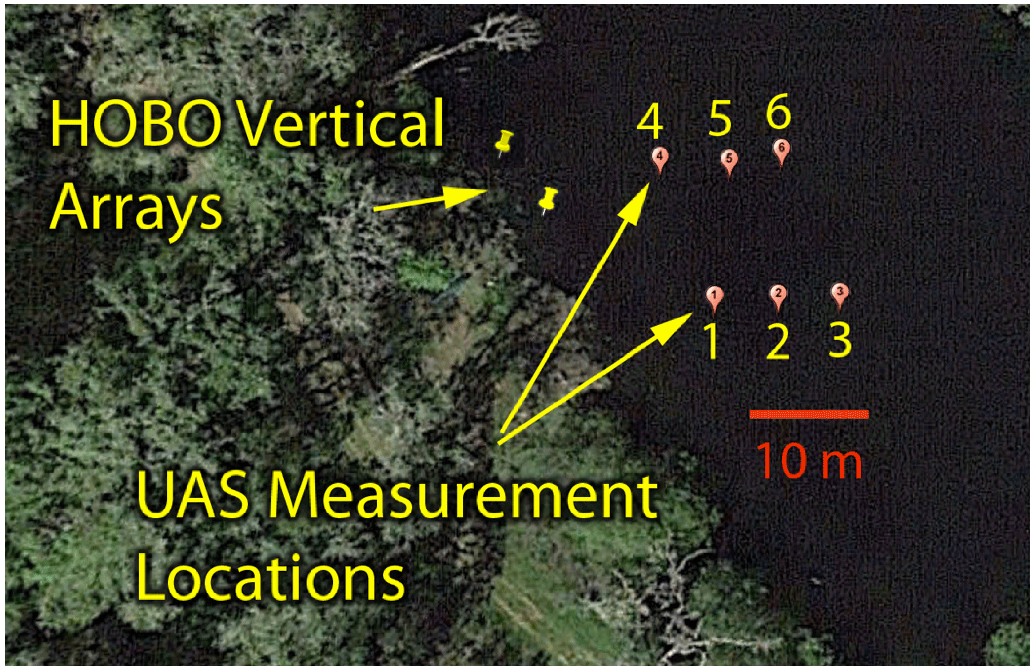
2.1. Site Description

Temperature sensing experiments were undertaken at Big Lake in Blue Oak Ranch Reserve (BORR), a 1330-ha undeveloped ecological reserve managed as part of the University of California’s Natural Reserve System. BORR is a locus for the development of ecological sensing technologies and was considered an ideal site to test the UAS platform due to its remote location and multiple surface water habitats. Big Lake is the largest of the perennial ponds at BORR. It has a surface area of 1.25 ha and a maximum depth of nearly 9 m.

Two vertical arrays of temperature sensors (6.5 m apart) were installed 10 m from the shoreline in 1.3 m water on the western boundary of the lake. Five HOBO Pendant temperature loggers were attached to the vertical array at depths of 0.25, 0.41, 0.56, 0.79 and 1.17 m. See Table 1 for sensor details.

Table 1. Sensor specifications.

Sensor	Specifications
In situ temperature	Hobo Pendant Temperature/Light Data Logger
	Resolution: 0.14 °C at 25 °C
	Accuracy: ±0.53 °C
	Operating range: −20–50 °C
Pressure-temperature	Measurement Specialties MS5803-01BA sensor
	Pressure resolution: 0.012 mbar
	Pressure accuracy: ±2.5 mbar
	Temperature resolution: 0.01 °C
	Water contact detector

Table 1. Sensor specifications.

Sensor	Specifications
In situ temperature	Hobo Pendant Temperature/Light Data Logger
	Resolution: 0.14 °C at 25 °C
	Accuracy: ±0.53 °C
	Operating range: −20–50 °C
Pressure-temperature	Measurement Specialties MS5803-01BA sensor
	Pressure resolution: 0.012 mbar
	Pressure accuracy: ±2.5 mbar
	Temperature resolution: 0.01 °C
	Water contact detector

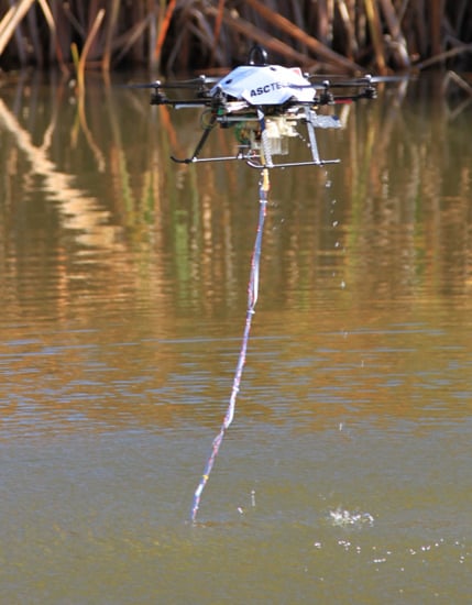
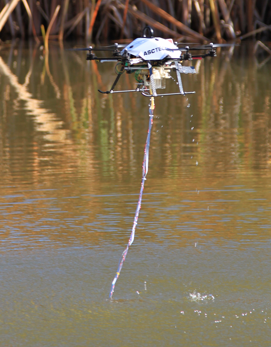
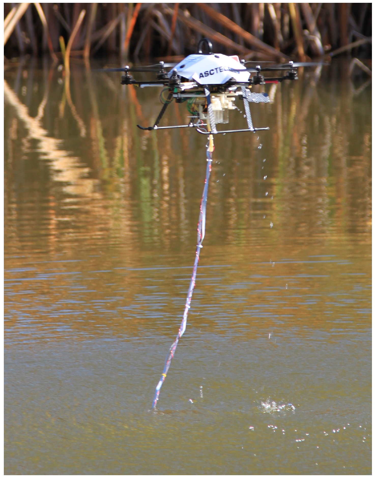
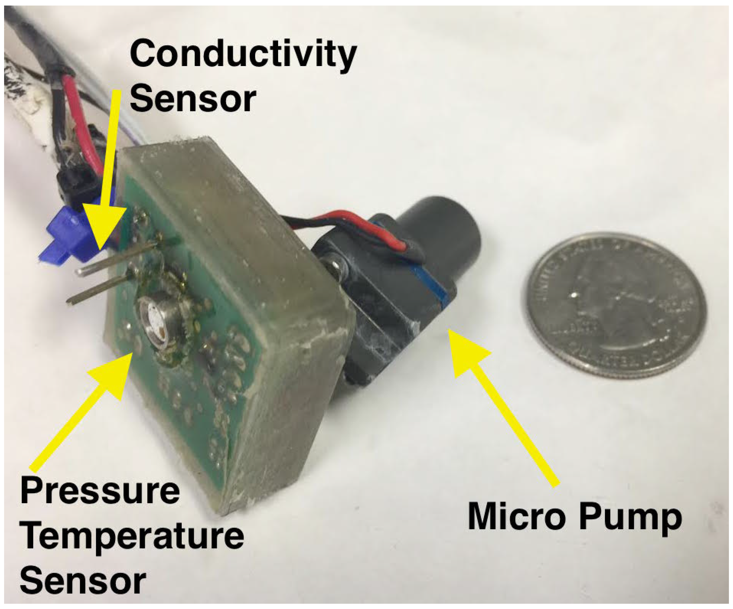
2.2. Vehicle and Sensors

Figure 1 shows the UAS system in flight at BORR. The UAS platform used in these experiments was an Ascending Technologies FireFly [37] Hexrotor with a 600-g payload and a flight time of approximately 20 min. The FireFly is equipped with a variety of sensors to measure position: a GPS, an inertial measurement unit and a pressure altimeter. The vehicle is controlled by input from two 802.15.4 XBee 2.4 GHz radios: one radio channel provides input from a remote control station on a laptop (allowing, for example, a pre-programmed flight path to be sent to the UAS) and another for manual control by a human pilot.

Figure 1. UAS in flight at Blue Oak Ranch Reserve.

Figure 1. UAS in flight at Blue Oak Ranch Reserve.

To facilitate the use of the UAS for freshwater ecology, we augmented the base platform with several sensors and subsystems [34]. Most importantly, we added multiple downward-facing ultrasonic rangers (Maxbotix MB1240-EZ4: ±1-cm accuracy within 2 m) to improve altitude estimation over water and thus provide better flight elevation control. To enable sensing within the water column, we attached a custom-built pressure-temperature embedded sensor system to a 4-m tube, which terminates in a pump, allowing water samples to also be made with the same system. A basic conductivity sensor is also attached to the end of the tube, allowing a direct indication of whether it is submerged or in air. This is primarily a safety feature to protect the pump and to ensure that it is submerged before pumping. A schematic of the system is shown in Figure 2, and the sensor specifications are provided in Table 1. During flight, the tube is reeled into the UAS, using a thin thread that runs through clips. The clips are attached to the tube at 0.75-m intervals, and the tube is retracted by spooling the thread beneath the UAS, causing the tube to coil below the vehicle. A long length of tube can become entangled in the environment, and its swinging motion during flight can induce dangerous and unstable flight dynamics. Therefore, the spooling mechanism reduces the hazards associated with flying with an object attached to the UAS.

To make measurements, the UAS hovers above the water surface, and the tube is extended through the water column. Varying water depths can be sampled either by changing the length of the tube that is extended into the water column or by changing the UAS altitude with a fixed length of tube extended. For each flight, the data from the UAS’s pressure-temperature system are transmitted from the UAS to a laptop ground station, where it is time stamped and written to a data log along with the UAS’s GPS coordinates and altitude.

Figure 2. Detail of the pressure-temperature embedded sensor system contained at the end of the UAS tube. A U.S. quarter piece is shown for scale.

Figure 2. Detail of the pressure-temperature embedded sensor system contained at the end of the UAS tube. A U.S. quarter piece is shown for scale.

2.3. Flights for Temperature Sampling

To compare temperature measurements from the UAS and in situ sensors, we made four flights. The fully-unspooled tube and thermal sensor were lowered through the water column near (∼0.5-m radius) one in situ thermal array, while maintaining a maximal distance from the other array. Temperatures were recorded at 4 Hz for 30 s at each of the five points through the water column, at 0.2-m intervals from 0.2 m deep from the bed of the lake. We waited 30 min between flights to allow the array to re-equilibrate to the background value. We selected 30 min because we previously confirmed that this duration was sufficient to achieve equilibrium following a disturbance. Flights were made in the late afternoon of 20 March 2015, with an average air temperature of 18 °C and a wind speed of 2.1 m/s. A comparison of these conditions with in situ temperature logging made during the preceding days indicated that the water column experienced mild diurnal temperature variances, with no evidence of over-turning or significant change in the surface mixed layer depth. Due to these stable, stratified conditions, we did not expect to observe exaggerated temperature dynamics in the lake during the experiments.

Data from the in situ array and the UAS were post-processed as described in Section 2.4 and compared for each flight.

To explore the feasibility of larger scale mapping with the UAS, we made two flights, using the spooling mechanism, to measure vertical profiles at three points along two parallel lines, as shown in Figure 3. The two parallel lines are separated by 10 m, with points in each line spaced 5 m apart. We flew ∼4 min at each location, starting at a higher altitude to submerge the pressure-temperature sensor to a shallow depth of ∼0.5 m, then descending by 0.5-m increments every 30 s. After eventually submerging and holding the sensor at a maximum depth of ∼2.5 m at each location, we ascended high enough to completely clear the water, then flew to the next location.

Figure 3. Locations of vertical profile measurements made by the UAS at Big Lake, Blue Oak Ranch Reserve, California, USA.

Figure 3. Locations of vertical profile measurements made by the UAS at Big Lake, Blue Oak Ranch Reserve, California, USA.

2.4. Post-Processing

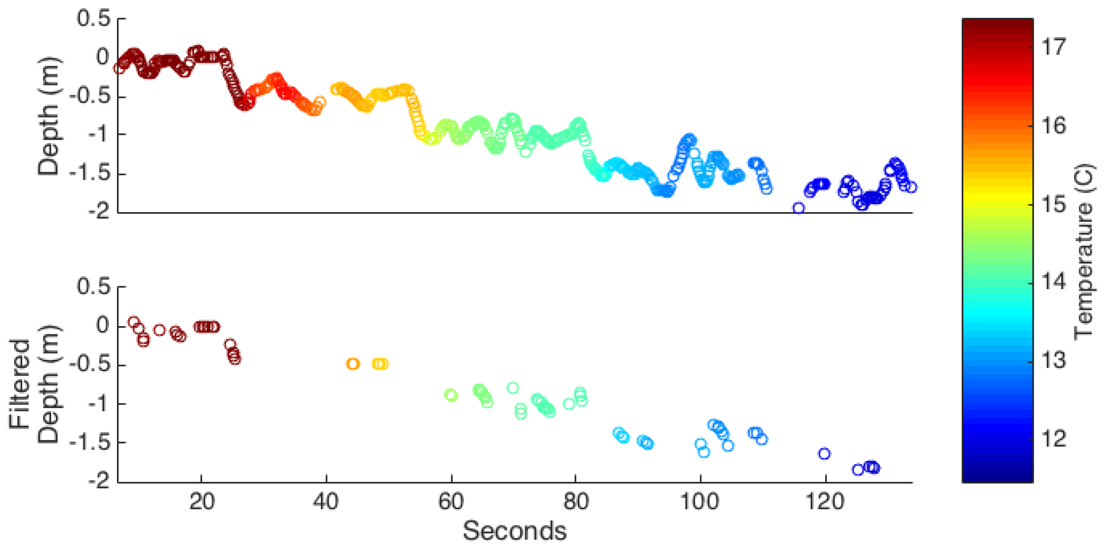
Post-processing involved two steps: filtering UAS temperature data and calibrating the UAS and in situ sensors to a common temperature datum.

2.4.1. Filtering

We filtered the temperature data because unintentional altitude changes in the UAS during flight result in the temperature sensor moving periodically up and down 25 cm through the water column. This movement causes multiple temperature readings to be associated with a given target depth and is problematic because the thermal response time of the MS5803 sensor is long compared to the rate of vertical movements. On average, the sensor requires 90 ± 45 s to converge to 90% of the actual temperature (the temperature response time of the sensor system is slowed due to polyurethane waterproofing that protects the electronics). To avoid erroneous data associated with these long equilibration times, we filtered the temperature data based on the joint rates of the change of pressure sensor depth and temperature. Specifically, we excluded temperature readings when either temperature or depth changes quickly: $\left|\frac{\partial T}{\partial t}\right|\ge 0.04°\text{C}{s}^{-1}$ or $\left|\frac{\partial m}{\partial t}\right|\ge 0.35{\mathrm{ms}}^{-1}$. These thresholds were determined by visually inspecting plots of the temperature and depth rates of change and observing that during periods of minimal change, nearly all values are bounded by the aforementioned thresholds. As shown in Figure 4, this filtering method retained 15% of the original readings and discarded most readings from the descent periods between the five measurement points in the water column.

Figure 4. The filtering method removes data when temperature and depth change rapidly.

Figure 4. The filtering method removes data when temperature and depth change rapidly.

2.4.2. Calibration

Prior to comparing UAS and in situ temperature readings, we calibrated the sensors against each other in the laboratory using room temperature water (21.8 °C) and ice water (0.1 °C). The MS5803 (UAS) sensor reported higher temperatures than the HOBO (in situ) sensor, except during periods of rapid temperature change, when the two sensors reported comparable values. We assumed that temperature changes imposed during calibration would be large compared to temperature changes measured in the field and therefore adjusted the UAS temperature data to improve correspondence with the in situ sensor readings obtained during calibration. The UAS temperatures were offset by −0.3 °C.

3. Results and Discussion

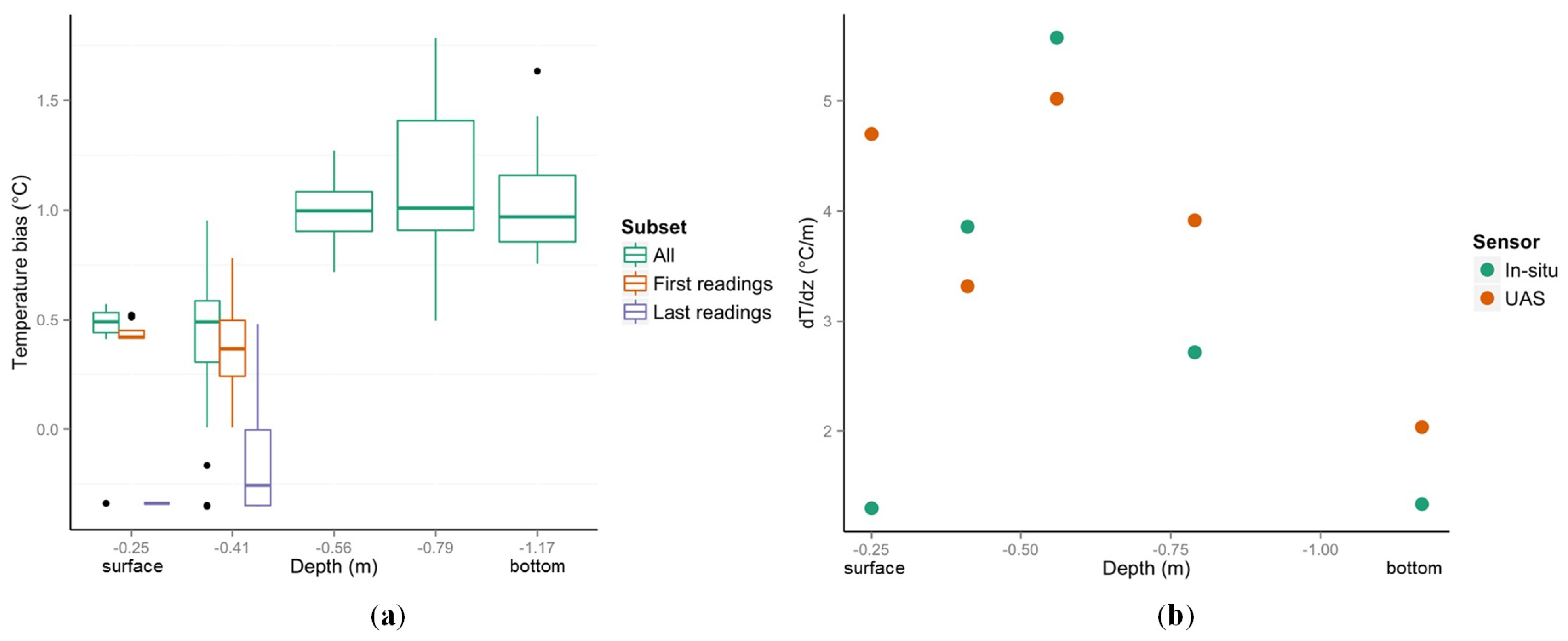
3.1. Comparison of UAS and In Situ Temperature Measurements

Over the four test flights, the UAS sensors reproduced the temperature variations in space associated with the water column’s thermal gradient and the mean variations in time during the two-hour experimental window. However, the temperatures measured from the UAS were consistently higher than the in situ array-recorded temperatures, even following calibration. The magnitude of the temperature bias varied with depth in the water column and was highest in deeper areas of the water column. Figure 5 shows box plots of the bias associated with each temperature measurement made by the UAS over the four flights, binned by depth in the water column. The bias is on the order of 0.5 °C in the surface 0.5 m of the water column and increases to 1 °C at greater depths below the thermocline.

While it is encouraging that these deviations in temperature are comparable to those made by other methods (e.g., TIR [24]; fiber optics [23,38]), the deviations are much greater than previously seen in mobile sensing systems [30]. Furthermore, the depth dependence in the magnitude of the bias suggests that a physical mechanism may be responsible. We hypothesized that several mechanisms could explain the bias: thermal lag effects when the sensor was first introduced into the water column from the air or entrainment of cold water from a depth to surface layers as the sensor was raised from the lake bed to the surface. As a preliminary means to distinguish between these hypotheses, we explored whether the magnitude of the thermal bias at the surface varied between the first shallow readings and the final readings made during a flight.

As seen in Figure 5, the UAS sensor temperatures remain higher than the in situ sensor temperatures near the surface, but the bias is decreased in the first readings during a flight. The direction of the bias switches for the final shallow readings during a flight, with temperatures measured from the UAS being lower than the in situ array-recorded temperatures. We suggest that these observations are more consistent with the entrainment of cold water as the tube and sensor were moved up through the water column at the end of a flight, than with the effect of thermal lags. Thermal lags in the onboard UAS sensor would be expected to have led to large positive biases in temperature upon initial entry into the water column. Despite the temperature bias between the UAV and in situ sensors, the UAV sensor’s temperature resolution of 0.01 °C is sufficient for capturing fine-scale thermal heterogeneities in the water column.

Figure 5. Comparison of UAS-borne and in situ temperature sensors, including logged data and detected thermal gradient. (a) Bias in temperature measured at each depth; (b) comparison of the derived temperature gradient at each depth.

Figure 5. Comparison of UAS-borne and in situ temperature sensors, including logged data and detected thermal gradient. (a) Bias in temperature measured at each depth; (b) comparison of the derived temperature gradient at each depth.

To remove systematic bias from the temperature sensors during the field trials and to consider only relative variations in temperature, we also compared estimates of the local thermal gradient in the water column as made from each of the sensing platforms, presenting the results in Figure 5. Below the water surface, both platforms produced comparable trends in the thermal gradient, again within 0.5–1 °C m${}^{-1}$ of each other. Both the peak in the thermal gradient associated with the thermocline, at a depth of approximately 0.6 m, and increased thermal stability with depth were identified by both sensor platforms. Significant disagreement between the measurements was only observed in the top 0.25 m of the water column, when the UAS measurements indicate a peak in thermal gradient comparable to that at the thermocline, while the in situ sensors indicate a fairly consistent temperature change with depth. The source of this high temperature gradient as sensed by the UAS is not completely resolved, but may be associated with a lack of elevation stability, causing the sensor to be suddenly pulled out of the water when at the surface and to undergo a rapid temperature change.

3.2. What Water Column Disturbance Is Induced by the UAS?

We hypothesized that water column disturbance induced by the UAS due to propeller wash and the motion of the tube would result in greater mixing and, thus, higher variance in temperatures measured below the UAS compared to a control. First, we confirmed that temperature variance measured at a given depth did not depend on the time window over which variance was calculated. We then computed temperature variances over 30-s periods for all depths and compared the profiles of the temperature variance at the test and control temperature arrays with a paired t-test. We did not find a significant difference in the temperature variances at any depth (p > 0.05), except for the shallowest in situ sensor depth: t = −2.53, p = 0.01. This suggests that any disturbance caused by the UAS in the water column is comparable in magnitude to natural sources of perturbation in the water profile. However, increased temperature variance at the surface of the water column provides evidence of UAS-induced disturbances due to propeller wash or mixing from the sensor occasionally being pulled out of the water.

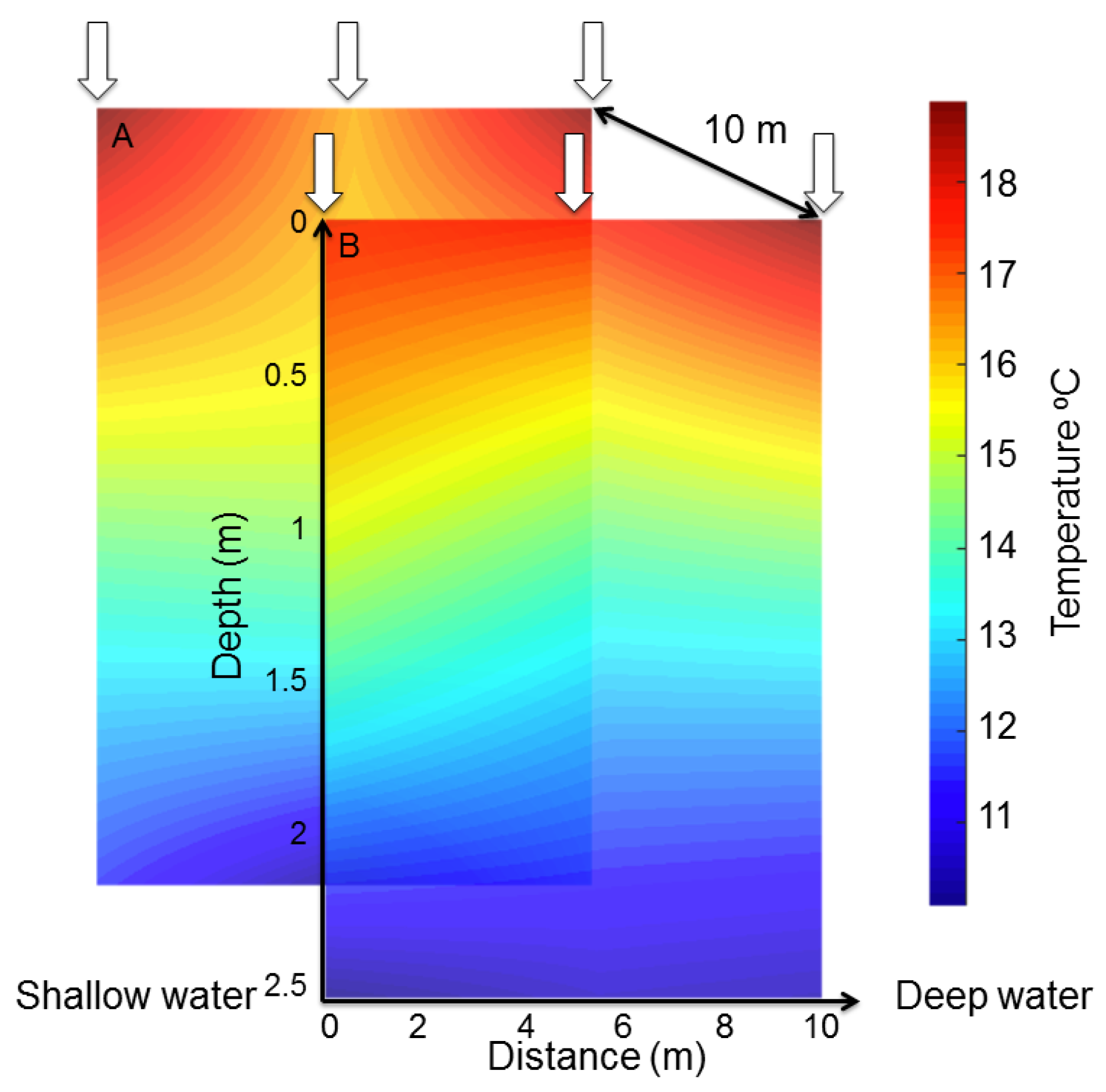
3.3. Feasibility of Mapping 3D Temperature Structure

Figure 6 illustrates the interpolated temperature structure in a 10 × 10 × 2.5 m region of Big Lake. The UAS sensors allowed multiple sites and depths to be measured on a fine grid. The platform also resolved the thermal structure of Big Lake, including vertical trends and the more subtle lateral trends, specifically a general decrease in temperature away from shore. Obtaining these 30 data points required 26.5 min of flight time during two UAS flights, plus time for setup and deployment.

While still faster than some manual techniques, rapid development of comprehensive spatial maps over large areas with short time frames will require further advances. The obvious technical limitations include battery life, which, coupled with the relatively slow response time of the thermal sensors used, limited the number of locations that could be sampled per flight. Thermal sensors better suited to this application are available, and future deployments will focus on a thermocouple with response times of 5 s or less [39]. Using such a sensor, the UAS could measure temperatures every 0.5 m at depths from 0–4 m at twenty different sampling locations within the 18 min battery life. At this rate, approximately five flights would be needed to measure Big Lake on a 10 × 10 m grid. This would be achievable in under 2 h, and repeat flights would be sufficient to allow diurnal cycling to be resolved.

Figure 6. Thermal structure of a 10 × 10 × 2.5 m grid, interpolated and reconstructed from two UAS flights. White arrows indicate the UAS’s sampling locations; depth measurements were made throughout the water column at these sites.

Figure 6. Thermal structure of a 10 × 10 × 2.5 m grid, interpolated and reconstructed from two UAS flights. White arrows indicate the UAS’s sampling locations; depth measurements were made throughout the water column at these sites.

Use of the UAS platform, as with other mobile sensing methods, presents a tradeoff between the detailed information from the high spatial resolution of temperature measurements and the limitations of a discontinuous time frame in which measurements are taken. While in situ sensors provide a temporally-continuous record of temperature at a location, the UAS captures a snapshot of the thermal structure in time. To account for general trends in temperature changes over time and a large area, sampling on a less dense grid may be necessary to avoid spatial biases, because the time frame of measurement is significantly longer than the time frame of temperature adjustment. For high resolution sampling with a single UAS, a nested sampling grid approach may be appropriate: the UAS could be flown to points on a less dense grid to record an initial thermal structure, then flown to points on subsections of a denser grid during shorter, constrained flight times to avoid any significant warming or cooling during the flight. Data from a small set of in situ temperature loggers could then be incorporated to detrend warming during the flight time period; in practice, we expect to use both in situ and UAS sensors.

The quality of the resulting data and the ease of deployment would be enhanced by improved sensor calibration and improvements in stabilizing the UAS with respect to drift and altitude variation. Because this was an initial evaluation of the UAS platform’s temperature probing capabilities, the sample size used in the experiment is not very large. To further assess the accuracy of this methodology, we plan to incorporate a new onboard thermocouple with a faster response time and to compare its measurements with in situ sensors to calibrate accordingly. Additionally, the latest commercially-available UASs are characterized by improved stability and altitude control, which would address these issues, and we expect that UAS and battery technology will continue to improve.

3.4. Operational Modes

The temperature readings were made using two different modes of flight: (1) flying down to within 1.2 m of the water surface, then unspooling the tube while hovering; and (2) flying with a completely unspooled tube and approaching the water from a higher altitude. We found no clear differences in the disturbances induced in the in situ lake temperatures between the flight modes, but made some operational observations. Specifically, flying with an unspooled tube enabled the UAS to remain high above the water surface. This offered a safer flight mode by increasing the buffer distance between the vehicle and lake and reducing the visual disturbance of the lake surface. However, altitude variation was more pronounced in this flight mode (typically above 1.8 m). At these altitudes, the UAS relies on a barometric altitude sensor that drifts due to wind and the continual natural variation in ambient air pressure. We often observed changes of ±0.2 m within less than a minute. However, when flying closer to the water surface (within 1.8 m), the UAS uses short distance ultrasonic rangefinders that enable steadier flight. In practice, we would recommend flying farther from the water to reduce operational stress on UAS pilots.

3.5. Pragmatic Limitations

Technological challenges aside, researchers must navigate a volatile regulatory landscape that varies by country [40,41]. Recently, some countries have proposed rules governing the use of UASs by academic researchers that are focused on limiting payload, altitude, visual range and proximity to densely-populated areas [42]. Researchers seeking official sanction should allow ample time to address local regulations or risk derailing a project’s timeline for data collection. Clearer and simpler regulations for environmental sensing with UASs in low-risk, low-altitude and low-population areas would increase their practicality and usefulness.

4. Conclusions

This paper outlines a novel method using a UAS to characterize the thermal structure in shallow bodies of water. The preliminary experiments illustrate that physically lowering a sensor from air with a UAS can obtain reliable and robust measurements of ambient water temperature, with reasonable agreement with in situ measurements and without significantly disturbing the water column. The results suggest that operationally, the best results are obtained when a sensor is lowered into the water column from an unspooled tube. Furthermore, the most reliable measurements are made when the elevation change of the sensor is slow and the sensor is descending. Future research should focus on improving the UAS elevation stability and minimizing drift, along with incorporating faster temperature sensors to capture the thermal structure with high resolution even when moving quickly through the water. With improved temperature sensors, as many as twenty 4-m surface water profiles could be obtained in a single 18-min flight. This would be fast enough to allow multiple flights to capture key diurnal variations and sufficient to allow complete characterization of small water bodies (circa 1 ha) in less than two hours. Although the system tested here focused on a small lake, the aerial platform could be used to characterize the thermal structure and regimes in streams, rivers, wetlands and larger lake systems.

References

1. Caissie, D. The thermal regime of rivers: A review. Freshw. Biol. 2006, 51, 1389–1406. [Google Scholar] [CrossRef]
2. Alabaster, J.S.; Lloyd, R.S. Water Quality Criteria for Freshwater Fish; Elsevier: London, UK, 2013. [Google Scholar]
3. Jankowski, T.; Livingstone, D.M.; Buhrer, H.; Forster, R.; Niederhauser, P. Consequences of the 2003 European heat wave for lake temperature profiles, thermal stability, and hypolimnetic oxygen depletion: Implications for a warmer world. Limnol. Oceanogr. 2006, 51, 815–819. [Google Scholar] [CrossRef]
4. Mooji, W.M.; Hulsmann, S.; de Senerpont Domis, L.N.; Nolet, B.A.; Bodelier, P.L.E.; Boers, P.C.M.; Pires, M.D.; Gons, H.J.; Ibelines, B.W.; Noordhuis, R.; et al. The impact of climate change on lakes in the Netherlands: A review. Aquat. Ecol. 2005, 39, 381–400. [Google Scholar] [CrossRef]
5. Bowler, D.E.; Mant, R.; Orr, H.; Hannah, D.M.; Pullin, A.S. What are the effects of wooded riparian zones on stream temperature? Environ. Evid. 2012, 1, 1–9. [Google Scholar] [CrossRef]
6. Vannote, R.L.; Sweeney, B.W. Geographic analysis of thermal equilibria: a conceptual model for evaluating the effect of natural and modified thermal regimes on aquatic insect communities. Am. Nat. 1980, 115, 667–695. [Google Scholar] [CrossRef]
7. Ward, J.V.; Stanford, J.A. Thermal responses in the evolutionary ecology of aquatic insects. Annu. Rev. Entomol. 1992, 27, 97–117. [Google Scholar] [CrossRef]
8. Wilby, R.L.; Orr, H.; Watts, G.; Battarbee, R.W.; Berry, P.M.; Chadd, R.; Dugdale, S.J.; Dunbar, M.J.; Elliott, J.A.; Extence, C.; et al. Evidence needed to manage freshwater ecosystems in a changing climate: Turning adaptation principles into practice. Sci. Total Environ. 2010, 408, 4150–4164. [Google Scholar] [CrossRef] [PubMed]
9. Tonolla, D.; Acuna, V.; Uehlinger, U.; Frank, T.; Tockner, K. Thermal heterogeneity in river floodplains. Ecosystems 2010, 13, 727–740. [Google Scholar] [CrossRef]
10. Lewis, Q.W.; Rhoads, B.L. Rates and patterns of thermal mixing at a small stream confluence under variable incoming flow conditions. Hydrol. Process. 2015, 29, 4442–4456. [Google Scholar] [CrossRef]
11. Rice, S.P.; Kiffney, P.; Greene, C.; Pess, G.R. The ecological importance of tributaries and confluences. In River Confluences, Tributaries and the Fluvial Network; Rice, S., Roy, A., Rhoads, B., Eds.; John Wiley & Sons: Chichester, UK, 2008. [Google Scholar]
12. Ebersole, J.L.; Liss, W.J.; Frissell, C.A. Cold water patches in warm streams: Physicochemical characteristics and the influence of shading. JAWRA J. Am. Water Resour. Assoc. 2003, 39, 355–368. [Google Scholar] [CrossRef]
13. Holtby, L.B. Effects of logging on stream temperatures in Carnation Creek, British Columbia, and associated impacts on the coho salmon (Oncorhynchus kisutch). Can. J. Fish. Aquat. Sci. 1988, 45, 502–515. [Google Scholar] [CrossRef]
14. Torgersen, C.E.; Price, D.M.; Li, H.W.; McIntosh, B.A. Multiscale thermal refugia and stream habitat associations of chinook salmon in northeastern Oregon. Ecol. Appl. 1999, 9, 301–319. [Google Scholar] [CrossRef]
15. Ruesch, A.S.; Torgersen, C.E.; Lawler, J.J.; Olden, J.D.; Peterson, E.E.; Volk, C.J.; Lawrence, D.J. Projected climate-induced habitat loss for salmonids in the John Day River network, Oregon, USA. Conserv. Biol. 2012, 26, 873–882. [Google Scholar] [CrossRef] [PubMed]
16. Wüest, A.; Lorke, A. Small-scale hydrodynamics in lakes. Annu. Rev. Fluid Mech. 2003, 35, 373–412. [Google Scholar] [CrossRef]
17. Romero, J.R.; Kling, G.W. Spatial-temporal variability in surface layer deepening and lateral advection in an embayment of Lake Victoria, East Africa. Limnol. Oceanogr. 2002, 47, 656–671. [Google Scholar] [CrossRef]
18. Oldham, C.E.; Sturman, J.J. The effect of emergent vegetation on convective flushing in shallow wetlands: Scaling and experiments. Limnol. Oceanogr. 2001, 46, 1486–1493. [Google Scholar] [CrossRef]
19. Horsch, G.; Stefan, H. Convective circulation in littoral water due to surface cooling. Limnol. Oceanogr. 1988, 33, 1068–1083. [Google Scholar] [CrossRef]
20. Michael, C.; John, F. The radiatively driven natural convection beneath a floating plant layer. Limnol. Oceanogr. 1994, 39, 1186–1194. [Google Scholar] [CrossRef]
21. Rinke, K.; Huber, A.M.R.; Kempke, S.; Eder, M.; Wolf, T.; Probst, W.N.; Rothhaupta, K.O. Lake-wide distributions of temperature, phytoplankton, zooplankton, and fish in the pelagic zone of a large lake. Limnol. Oceanogr. 2009, 54, 1306–1322. [Google Scholar] [CrossRef]
22. Moore, R.D.; Spittlehouse, D.L.; Story, A. Riparian microclimate and stream temperature response to forest harvesting: A review. J. Am. Water Resour. Assoc. 2005, 41, 813–834. [Google Scholar] [CrossRef]
23. Selker, J.S.; Thevenaz, L.; Huwald, H.; Mallet, A.; Luxemburg, W.; van de Giesen, N.; Stejskal, M.; Zeman, J.; Westhoff, M.; Parlange, M.B. Distributed fiber-optic temperature sensing for hydrologic systems. Water Resour. Res. 2006, 42, 1–8. [Google Scholar] [CrossRef]
24. Torgerson, C.E.; Faux, R.N.; McIntosh, B.A.; Poage, N.J.; Norton, D.J. Airborne thermal remote sensing for water temperature assessment in rivers and streams. Remote Sens. Environ. 2001, 76, 386–398. [Google Scholar] [CrossRef]
25. Handcock, R.N.; Gillespie, A.R.; Cherkauer, K.A.; Kay, J.E.; Burges, S.J.; Kampf, S.K. Accuracy and uncertainty of thermal-infrared remote sensing of stream temperatures at multiple spatial scales. Remote Sens. Environ. 2006, 100, 427–440. [Google Scholar] [CrossRef]
26. Jensen, A.M.; Neilson, B.T.; McKee, M.; Chen, Y. Thermal remote sensing with an autonomous unmanned aerial remote sensing platform for surface stream temperatures. In Proceedings of the 2012 IEEE International Geoscience and Remote Sensing Symposium, Munich, Germany, 22–27 July 2012; pp. 5049–5052.
27. Schmugge, T.J.; Kustas, W.P.; Ritchie, J.C.; Jackson, T.J.; Rango, A. Remote sensing in hydrology. Adv. Water Resour. 2002, 25, 1367–1385. [Google Scholar] [CrossRef]
28. Kay, J.E.; Kampf, S.K.; Handcock, R.N.; Cherkauer, K.A.; Gillespie, A.R.; Burges, S.J. Accuracy of lake and stream temperatures estimated from thermal infrared images. J. Am. Water Resour. Assoc. 2005, 41, 1161–1175. [Google Scholar] [CrossRef]
29. Dunbabin, M.; Grinham, A.; Udy, J. An autonomous surface vehicle for water quality monitoring. In Proceedings of the Australasian Conference on Robotics and Automation (ACRA), Sydney, Australia, 2–4 December 2009; pp. 2–4.
30. Laval, B.; Bird, J.S.; Helland, P.D. An autonomous underwater vehicle for the study of small lakes. J. Atmos. Ocean. Technol. 2000, 17, 69–76. [Google Scholar] [CrossRef]
31. Zhang, Y.; Godin, M.A.; Bellingham, J.G.; Ryan, J.P. Using an autonomous underwater vehicle to track a coastal upwelling front. IEEE J. Ocean. Eng. 2012, 37, 338–347. [Google Scholar] [CrossRef]
32. Marouchos, A.; Muir, B.; Babcock, R.; Dunbabin, M. A shallow water AUV for benthic and water column observations. In Proceedings of the OCEANS 2015—Genova, Genoa, Italy, 18–21 May 2015; pp. 1–7.
33. Zhang, F.; Wang, J.; Thon, J.; Thon, C.; Litchman, E.; Tan, X. Gliding robotic fish for mobile sampling of aquatic environments. In Proceedings of the IEEE 11th International Conference on Networking, Sensing and Control, Miami, FL, USA, 7–9 April 2014; pp. 167–172.
34. Ore, J.P.; Elbaum, S.; Burgin, A.; Detweiler, C. Autonomous Aerial Water Sampling. J. Field Robot. 2015. [Google Scholar] [CrossRef]
35. Hardin, P.J.; Jensen, R.R. Small-scale unmanned aerial vehicles in environmental remote sensing: Challenges and opportunities. GISci. Remote Sens. 2011, 48, 99–111. [Google Scholar] [CrossRef]
36. Dunbabin, M.; Marques, L. Robots for environmental monitoring: Significant advancements and applications. IEEE Robot. Autom. Mag. 2012, 19, 24–39. [Google Scholar] [CrossRef]
37. Achtelik, M.C.; Doth, K.M.; Gurdan, D.; Stumpf, J. Design of a Multi Rotor MAV with regard to Efficiency, Dynamics and Redundancy. In Proceedings of the AIAA Guidance, Navigation, and Control Conference (AIAA), Minneapolis, MN, USA, 13–16 August 2012; pp. 1–17.
38. Tyler, S.W.; Selker, J.S.; Hausner, M.B.; Hatch, C.E.; Torgerson, T.; Thodal, C.E.; Schladow, S.G. Environmental temperature sensing using Raman spectra DTS fiber-optic methods. Water Resour. Res. 2009, 45. [Google Scholar] [CrossRef] [Green Version]
39. Garnier, B.; Lanzetta, F. Tutorial 4: In situ Realization/Characterization of Temperature/Heat Flux Sensors; Technical Report; Université de Nantes: Nantes, France, 2011. [Google Scholar]
40. Mulero-Pázmány, M.; Stolper, R.; van Essen, L.; Negro, J.J.; Sassen, T. Remotely piloted aircraft systems as a rhinoceros anti-poaching tool in Africa. PLoS ONE 2014, 9. [Google Scholar] [CrossRef]
41. Vincent, J.B.; Werden, L.K.; Ditmer, M.A. Barriers to adding UAVs to the ecologist’s toolbox: Peer-reviewed letter. Front. Ecol. Environ. 2015, 13, 74–75. [Google Scholar] [CrossRef]
42. Whitehead, K.; Hugenholtz, C.H. Remote sensing of the environment with small unmanned aircraft systems (UASs), part 1: A review of progress and challenges. J. Unmanned Veh. Syst. 2014, 2, 69–85. [Google Scholar] [CrossRef]