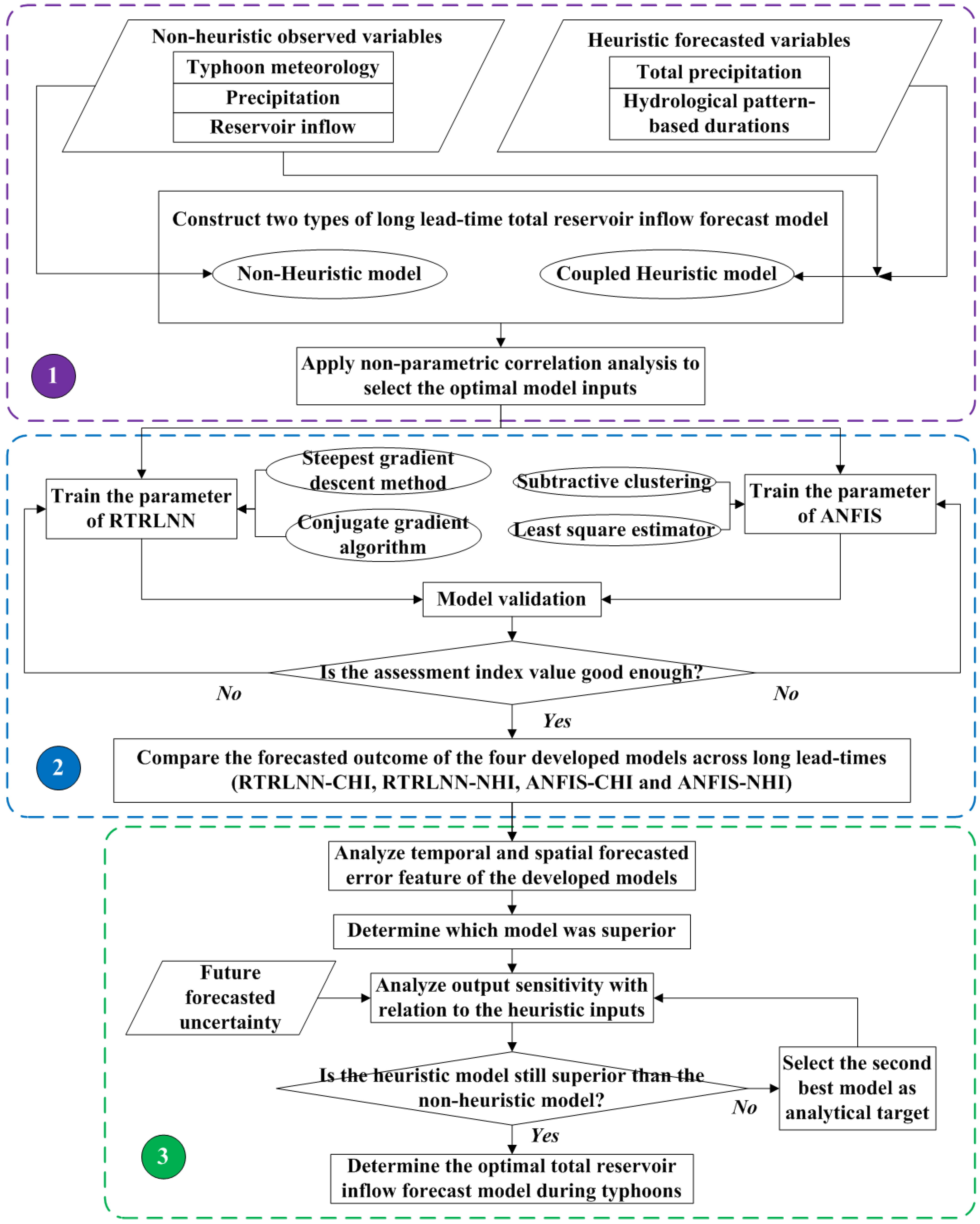
Article

Coupled Heuristic Prediction of Long Lead-Time Accumulated Total Inflow of a Reservoir during Typhoons Using Deterministic Recurrent and Fuzzy Inference-Based Neural Network

1
Department of Civil Engineering, National Taiwan University, No. 1, Sec. 4, Roosevelt Road, Taipei 10617, Taiwan
2
Department of Marine Environmental Informatics, National Taiwan Ocean University, No.2, Beining Rd.; Jhongjheng District, Keelung City 20224, Taiwan
*
Author to whom correspondence should be addressed.
Water 2015, 7(11), 6516-6550; https://doi.org/10.3390/w7116516
Submission received: 31 July 2015 / Revised: 19 October 2015 / Accepted: 9 November 2015 / Published: 17 November 2015
(This article belongs to the Special Issue Use of Meta-Heuristic Techniques in Rainfall-Runoff Modelling)

Abstract

:
This study applies Real-Time Recurrent Learning Neural Network (RTRLNN) and Adaptive Network-based Fuzzy Inference System (ANFIS) with novel heuristic techniques to develop an advanced prediction model of accumulated total inflow of a reservoir in order to solve the difficulties of future long lead-time highly varied uncertainty during typhoon attacks while using a real-time forecast. For promoting the temporal-spatial forecasted precision, the following original specialized heuristic inputs were coupled: observed-predicted inflow increase/decrease (OPIID) rate, total precipitation, and duration from current time to the time of maximum precipitation and direct runoff ending (DRE). This study also investigated the temporal-spatial forecasted error feature to assess the feasibility of the developed models, and analyzed the output sensitivity of both single and combined heuristic inputs to determine whether the heuristic model is susceptible to the impact of future forecasted uncertainty/errors. Validation results showed that the long lead-time–predicted accuracy and stability of the RTRLNN-based accumulated total inflow model are better than that of the ANFIS-based model because of the real-time recurrent deterministic routing mechanism of RTRLNN. Simulations show that the RTRLNN-based model with coupled heuristic inputs (RTRLNN-CHI, average error percentage (AEP)/average forecast lead-time (AFLT): 6.3%/49 h) can achieve better prediction than the model with non-heuristic inputs (AEP of RTRLNN-NHI and ANFIS-NHI: 15.2%/31.8%) because of the full consideration of real-time hydrological initial/boundary conditions. Besides, the RTRLNN-CHI model can promote the forecasted lead-time above 49 h with less than 10% of AEP which can overcome the previous forecasted limits of 6-h AFLT with above 20%–40% of AEP.

1. Introduction

Taiwan is located in the path of typhoons as they move in from the Western Pacific, and as a result, three to five typhoons hit Taiwan annually [1,2]. As the basins of the reservoir in Taiwan are mostly steep-sided, the concentration time is especially short and the reservoir inflow is extremely high under typhoon-induced precipitation [3]. The frequency of typhoons that bring heavy rain has been growing due to climate change [4,5,6], and inflows are more frequently surpassing original design and construction standards. Therefore, effective methods of ameliorating typhoon-related disasters need to include non-engineered disaster prevention programs, such as effective disaster forewarning and associated response mechanisms, which include the ability to identify the disaster before it occurs. The optimal releasing strategies for flood control are to minimize the maximum release and maximize the final storage under the principles of avoiding dam failure and overflow from the upstream riverbank, and keeping the water level lower than the dead storage level. Hence, we can expect that an accurate accumulated total reservoir inflow forecast model plays a most important role in determining whether the releasing decision can achieve optimization for flood control.
However, previous research into real-time long lead-time accumulated total reservoir inflow forecast during typhoons has been scarce, and it has proved difficult to achieve effective and accurate results because of future meteorological-hydrological uncertainty. The traditional method to derive real-time forecasted reservoir inflow hydrographs and the corresponding accumulated total inflow is firstly to forecast the typhoon precipitation hyetograph, and then the reservoir inflow hydrograph of the entire typhoon event is derived from the rainfall-runoff model. This type of rainfall-runoff modeling has been examined in the fields of the hydrological approach [7,8,9,10,11,12] and statistical approach [13,14]. However, studies like those above, regarding the real-time precipitation hyetograph forecast of an entire typhoon event, are scarce, so efficient and accurate long lead-time accumulated total inflow forecast is still in urgent need of development.
The other method regarding inflow forecast is to directly predict short lead-time reservoir inflow, because the model inputs only consider the real-time observed meteorological-hydrological information. These related works have been categorized under both the hydrological approach [15,16,17] and the statistical approach which mostly applied artificial neural networks (ANNs) such as the back-propagation neural network (BPNN) [18,19,20,21,22], the state space neural network [23], the adaptive network-based fuzzy inference system (ANFIS) [24], the recurrent neural network (RNN) [21], support vector machine [1], and the radial basis function [2] as construction tools. The advantage of the short lead-time forecast is that it is fairly accurate in medium-low reservoir inflow, whereas the disadvantages are that (1) the effective forecasted lead-time is only 6 h; (2) the forecasted error in the high flow periods is high, within the range of 10% to 40% [1,2]; and (3) the time-lag circumstances of the forecasted flow rate of a longer forecasted lead-time are significant. The main reason is that the previous models do not consider future reliable meteorological-hydrological factors as inputs. The feasible inputs include the delays from the current moment to the various key moments on the rainfall-runoff hydrograph, the accumulated total precipitation, and the observed-predicted inflow increase/decrease rate (OPIID rate), etc. Besides, the above studies concluded that the forecasted ability of RNN and ANFIS is better than the traditional ANNs like BPNN, and they have the potential to simulate longer lead-time inflow with larger tolerance ability for input errors. Moreover, among various ANN models, Chang et al. (2002) [25] indicated that real-time recurrent learning neural networks (RTRLNN) possesses dynamic real-time recurrent routing mechanisms that can simulate time-varying systems effectively.
In summary, the previous models seldom can achieve a reservoir inflow forecast with a long lead-time of up to 48–72 h considering the future highly varied meteorology-hydrology uncertainty of a typhoon. Because of the powerful capability of ANNs to model any kind of nonlinear relationship between inputs and output through a series of transfer functions without the need to make assumptions in advance, in recent years, ANNs have been used increasingly in applications for modeling hydrological processes. The advantages of using ANNs include the ability to derive accurate and fast real-time short-term forecasts with low building costs. However, the development and application of accurate and effective ANN-based models that have the most potential for long lead-time real-time inflow forecast (e.g., RTRLNN and ANFIS) with the other advanced novel heuristic techniques in accumulated total inflow forecasts during typhoons is a subject that urgently requires development and scientific breakthrough.
The purpose of this study is to apply RTRLNN and ANFIS with specially devised novel heuristic inputs such as observed-predicted inflow increase/decrease rate (OPIID rate), total precipitation (TP), duration from current time to the time of maximum precipitation, and direct runoff ending (DRE) to develop heuristic-type long lead-time accumulated total reservoir inflow forecast models. This study also utilized temporal-spatial forecasted error feature analysis to assess the feasibility of the developed long lead-time RTRLNN- and ANFIS-based models, and conducted output sensitivity analysis of single/combined heuristic inputs to determine whether the developed heuristic model is superior to the non-heuristic model and whether it is vulnerable to the impact of future forecasted uncertainty and error on inputs.

2. Development of Methodology

2.1. Procedures

The procedures used in this study are divided into three steps as shown in Figure 1. The detailed procedures are thoroughly described as follows:
Figure 1. Flowchart of the methodology.
Water 07 06516 g001
Step 1: First, observed short lead-time meteorological-, precipitation-, and pattern-based reservoir inflow factors during previous typhoons were specified as non-heuristic candidate inputs, and future long lead-time total precipitation- and pattern-based duration factors were specified as heuristic inputs. The optimal inputs for the non-heuristic and heuristic typhoon total inflow forecast model were selected by using non-parametric statistical correlation analysis.
Step 2: The steepest gradient descent (SGD) and conjugate gradient algorithm (CG) were used to train the parameter of RTRLNN, and subtractive clustering (SC) with the least square estimator (LSE) were applied to train the parameter of ANFIS. On obtaining the best model by comparing the assessment index value of the individually developed model type, the forecasted outcome for the RTRLNN-CHI (Coupled Heuristic Inputs) model, RTRLNN-NHI (No Heuristic Inputs) model, ANFIS-CHI model, and ANFIS-NHI model were compared across long lead-times.
Step 3-1: The temporal and spatial forecasted error feature of the four best types of long lead-time models developed were respectively analyzed, and a superior model determined.
Step 3-2: The output sensitivity of single or combined heuristic inputs due to future forecast uncertainty of the selected candidate optimal model among the four model types was analyzed under the impact of input forecasted error. Following the assessment, the optimal total reservoir inflow forecast model during typhoons was determined.

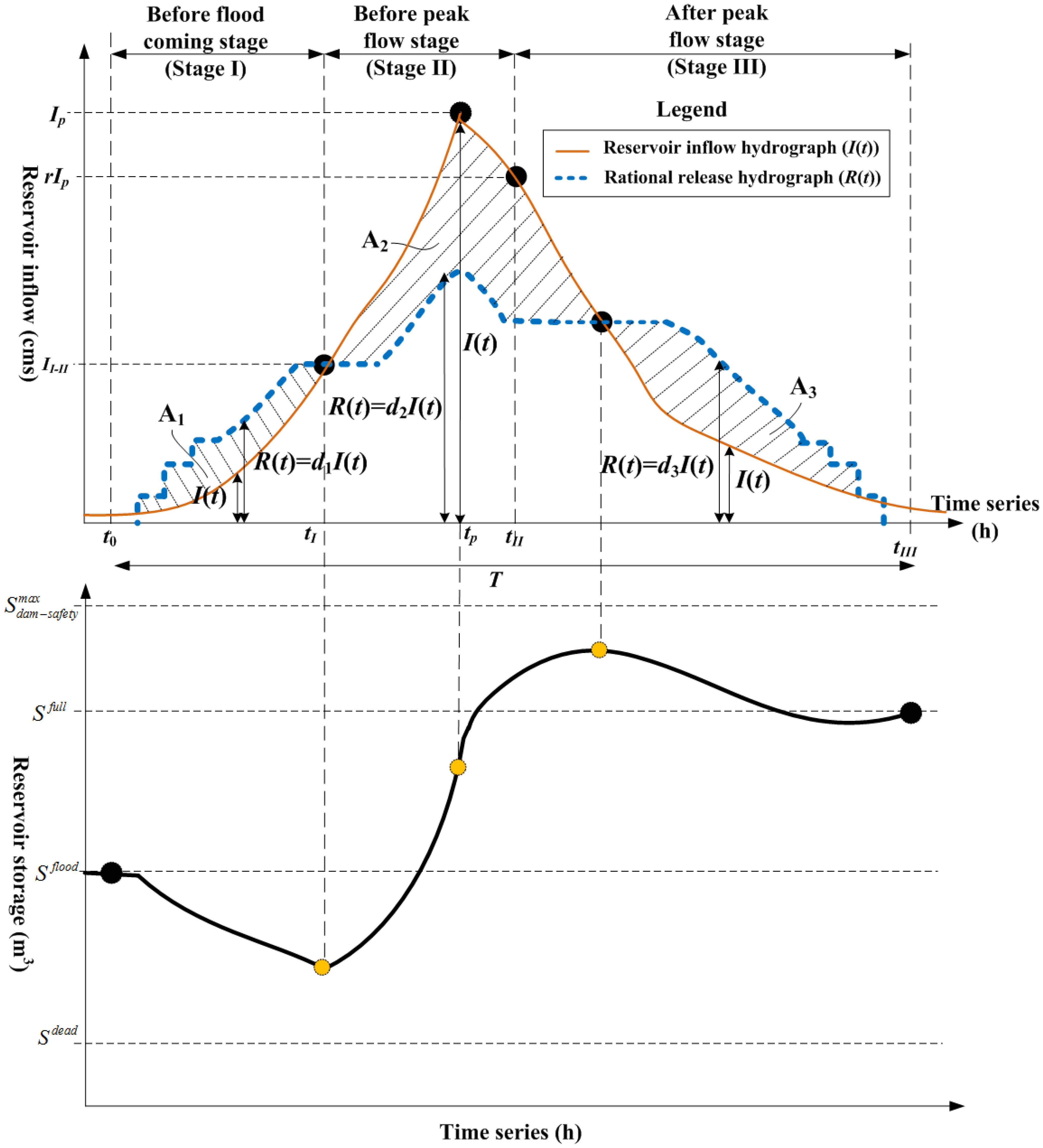
2.2. Developed Model Type of Accumulated Total Reservoir Inflow Forecast

This study designates the systematic operating mechanism of a reservoir of different stages as shown in Figure 2. To avoid dam failure and overflow from the upstream riverbank, the constraint can be expressed in Equation (1), and that to avoid a water level that is lower than dead storage is expressed in Equation (2).
A 2 A 1 < S d a m s a f e t y m a x x 0 S
A 1 < x 0 S S d e a d
where A1, A2, and A3 are the increasing/reducing storage of Stage I, increasing storage of Stage II, and increasing/reducing storage of Stage III, respectively; S d a m s a f e t y m a x is maximum safety storage for the dam; x 0 S is the initial storage; and S d e a d is the dead storage.
The releasing operating objectives of Stage I have to consider flood detention (expressed in Equation (3)) and final storage that at the same time (Equation (4)) are dominated by the future accumulated total inflow. Moreover, the constraint of Stage I involves avoiding the water level being lower than dead storage (Equation (2)). Hence, we can expect that the future accumulated total inflow is the key decision information of Stage I.
M a x { A 2 }
M i n { | A 1 + A 3 A 2 | | S f u l l x 0 S | }
where S d a m s a f e t y m a x is the maximum safety storage for the dam. In order to achieve optimal operation, the storage objective for the water supply is dominated primarily by Stage III and secondarily by Stage I, and the releasing operation of Stage II is used completely for flood detention (expressed in Equation (3)) that must subject to the safety constraint (Equation (1)). Hence, we can expect that the future total inflow is the key decision information of Stage II and Stage III.
Figure 2. Schematic diagram of the flood operating mechanism of different stages in conjunction with the reservoir inflow.
Water 07 06516 g002
The total reservoir inflow can be used as a criterion to determine the ideal amount of pre-discharge water and the benefit of flood detention under just filling the reservoir without overflowing the dam. Conventionally, the inflow can be calculated from the calculations of the rainfall-runoff simulation. The flow at the catchment outlet can be calculated using the unit hydrograph method, which is expressed as follows:
Q ( t ) = A 0 t P ( τ ) U ( t τ ) d τ d A
where Q ( t ) is the inflow at time t; P ( τ ) is the effective rainfall; and U ( t τ ) is the flow path unit response function. Liu et al. (2003) [26] estimated the travel time at an arbitrary point in the catchment area by combining the diffusive wave model with the flow path unit response function. Molnar and Ramirez (1998) [27] used Manning’s equation and energy dissipation theory to solve the approximate solutions to the diffusion waves, which can be expressed as follows:
U ( t ) = 1 σ 2 π t 3 t 0 3 exp [ ( t t 0 ) 2 2 π t t 0 ]
where t 0 is the average time of concentration for the water moving along the flow path from one point of the catchment area to the outlet; and σ is the standard deviation of the migration time. During the period of the typhoon, the effective rainfall in the future; P ( t + n ) , is related to the following atmospheric factors for the typhoon: distance between typhoon center and reservoir basin ( h c w ), grade 7/10 typhoon radius ( R ), typhoon movement speed ( v m ), central wind speed ( V max ), and central pressure ( p c ). It can be expressed as the following:
P ( t + Δ t ) = f ( h c w , R , v m , V max , p c )
where Δ t is the forecasted lead-time. However, the uncertainty of the meteorology-hydrology relationship over a long lead-time is too high to make a determination as to the future typhoon atmospheric factors ahead of time. It is difficult to accurately forecast the rainfall hyetograph of the entire typhoon event in the future.
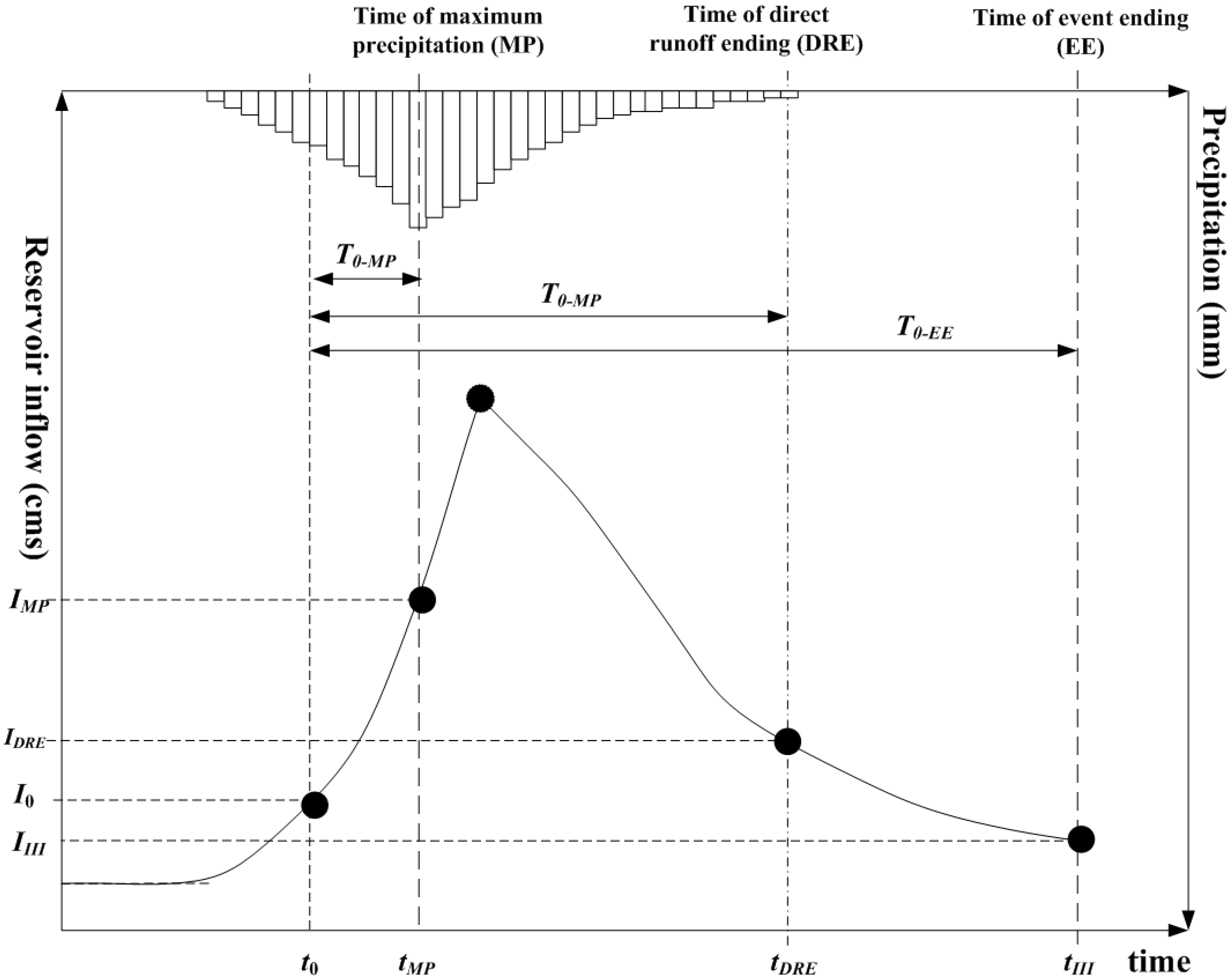
Hence, the rainfall-runoff model based on traditional hydrology was not used for real-time simulation and forecast of the reservoir inflow. A novel forecast method was developed and was found to be more reliable in forecasts. The new method adopted the total rainfall (Ptotal) method, and forecasted the various delays from the current moment to the key times along the rainfall-runoff hydrograph; for example, the delay from the current time to the maximum rainfall (T0-MP), the delay to the end of the direct runoff (T0-DRE), and the delay to the end of the water retreat (T0-EE). The new method also used the observed-predicted inflow increase/decrease rate (OPIID rate) as the heuristic-type input. It is expected to be able to simulate the total reservoir inflow of the runoff hydrograph from the rainfall trend from a certain typhoon moving path in the future. A schematic diagram of hydrological key points within the rainfall-runoff hydrograph is shown in Figure 3. In this study, an original and innovative forecast model for the total reservoir inflow was developed with heuristic forecast inputs using ANFIS and RTRLNN. The model developed was analyzed and compared with the non-heuristic forecast model in which the input only included the real-time observed meteorology and hydrology information. The feasibility of the heuristic model for real-time forecast was also evaluated.
Figure 3. Schematic diagram of hydrological key points within the rainfall-runoff hydrograph.
Water 07 06516 g003

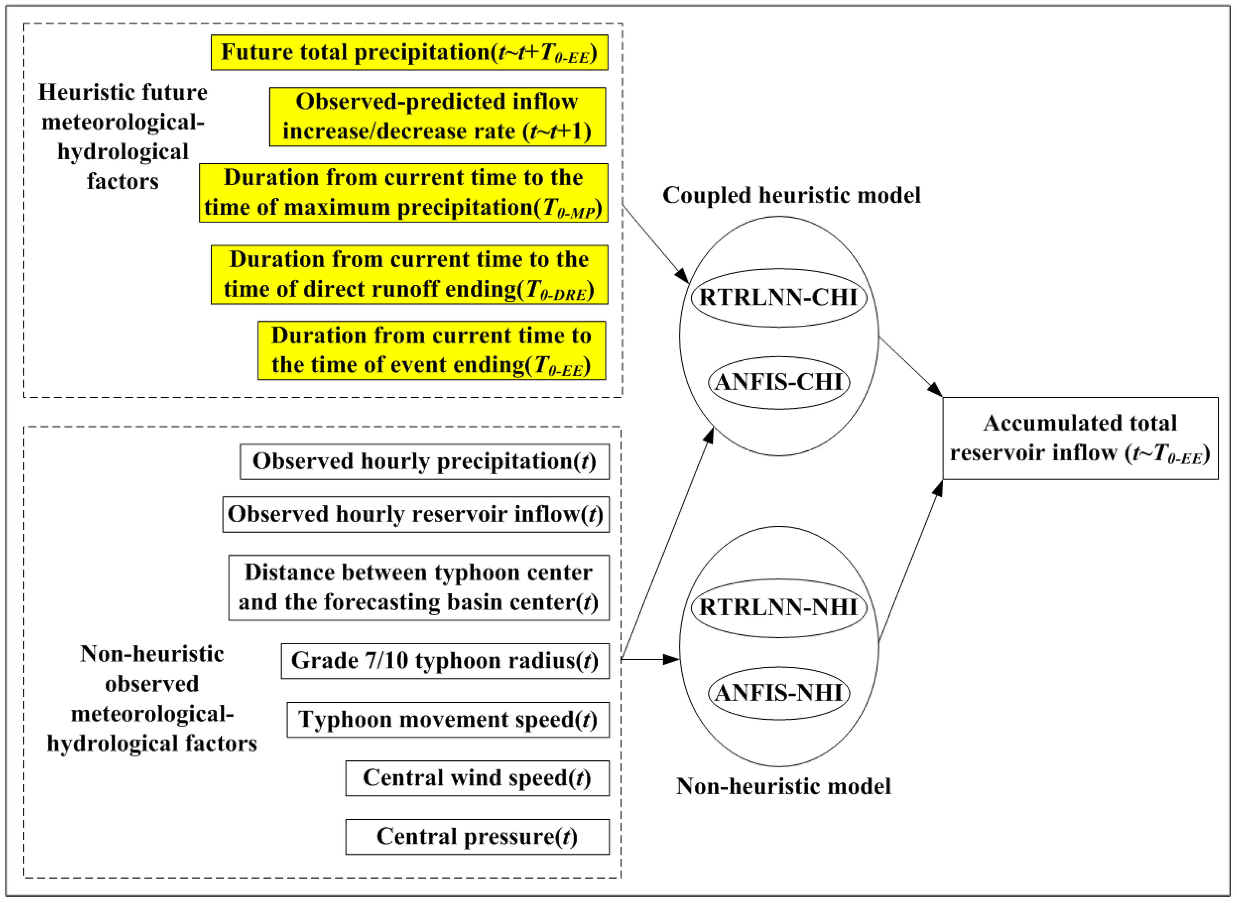
2.2.1. Candidate Predictor

The choice of input candidates for the model is based on the theory of computation for the rainfall-runoff characteristics of the meteorology-hydrology relationship, such as the variables of reference Equations (5)–(7). In this study, four types of predictors which can be observed and predicted in real-time were used:
(1) Typhoon meteorological factor: longitude, latitude, central wind speed, central pressure, grade 7 typhoon radius, grade 10 typhoon radius, and typhoon movement speed, etc. The other feasible alternatives include relative humidity and temperature of the typhoon and basin, etc., but the other feasible alternatives are relatively not highly related to inflow and were not selected as candidate inputs.
(2) Rainfall station factor: observed hourly rainfall and total precipitation at the ground station. The other feasible alternatives include radar reflective information and satellite image from the typhoon, but the accuracy and correlation toward surface rainfall is not as high as that of the ground station. Hence, the alternatives are not adopted as candidate inputs.
(3) The distance between the typhoon center and the forecasting basin center (d(t)): this distance can be obtained using a conversion formula from longitude/latitude to distance:
y ( t ) = 111.1 × ( l a t c ( t ) - l a t f o s ( t ) )  
x ( t ) = 111.1 × ( l o n c ( t ) - l o n f o s ( t ) ) × c o s ( l a t c ( t ) + l a t f o s ( t ) 2 )  
d ( t ) = ( x ( t ) ) 2 + ( y ( t ) ) 2
where l a t c ( t ) and l a t f o s ( t ) are the latitudes of the typhoon center and the forecasting basin center at time t, and l o n c ( t ) and l o n f o s ( t ) are longitudes of the typhoon center and the forecasting basin center at time t.
(4) Runoff factor:
I. The delays from the current moment to the various key moments on the rainfall-runoff hydrograph in hydrology. For example, these include the delay from the current moment to the moment the maximum rainfall occurs (T0-MP), the delay to the end of the direct runoff (T0-DRE), and the delay to the end of the water retreat (T0-EE). The feasible alternative includes the delay to the inflection point after peak flow, which is equal to the delay to rainfall excess ending plus the time of concentration. However, it is difficult to predict the delay to rainfall excess ending in real-time across a long lead-time, leading to this alternative not being adopted.
II. The real-time observed hourly reservoir inflow and the observed-predicted inflow increase/decrease rate (OPIID rate).
The total precipitation could be obtained by constructing a forecast database from the historical samples of the relationship between the center position of the typhoon and the rainfall in the catchment area using data mining techniques. Similarly, the delay of the future typhoon invasion could be obtained by constructing a forecast database from the historical samples of the distribution of the center position of the typhoon when the maximum rainfall occurred, the time when the direct runoff ended, and the time when the water retreated using data mining techniques. The above-mentioned heuristic inputs (total precipitation and delays) are estimated by the path and direction of the typhoon and the characteristic database. Besides, the output of the model was the total reservoir inflow during the period from the current moment to the end of the event. In this research, a heuristic forecast model was studied. The inputs to this heuristic model simultaneously comprised the real-time observed meteorology and hydrology information (typhoon characteristic factors, basin hourly precipitation, basin reservoir hourly inflow) and future forecasted heuristic meteorology and hydrology information (the total rainfall from the current moment to the end of the event, T0-MP,T0-DRE,T0-EE, and OPIID rate). The input for the non-heuristic forecast model only included the real-time observed meteorology and hydrology information. The structure of the developed heuristic-type and non-heuristic accumulated total inflow forecast model is shown in Figure 4.
Figure 4. Structure of the developed coupled heuristic and non-heuristic accumulated total inflow forecast model.
Water 07 06516 g004

2.2.2. Selection of Model Inputs

The feasible measures to select optimal model inputs include correlation analysis, principle component analysis, and the trial-and-error method. Among previous studies, the trial-and-error method is the most applied approach which is time-consuming. To effectively quantify the aptness for the large amount of candidate model inputs, this study uses correlation analysis for decision-making, and Spearman’s rank correlation coefficient [28] is adopted as an analysis index. The analysis mechanism used for the correlation depends on the rank relationship of the time-series of two variables, and hence, this analysis can determine the correlation and suitability of input, regardless of the kind of relationship that exists between the candidate input and output, that is,
r r a n k = 1 6 i = 1 n D i 2 n ( n 2 1 )
D i 2 = ( R a n k x i R a n k y i ) 2
where rrank is Spearman’s rank correlation coefficient, n is the number of data, x is the candidate input of the forecast model (predictor), y is the model output also known as the predictant (accumulated total reservoir inflow during time t + 1 to t + T0-EE), and R a n k x i and R a n k y i are the sort values of xi and yi in their individual time-series of the variable, respectively. The most correlated candidate predictors for forecasting accumulated total inflow will be selected as optimal inputs, and the selected inputs must subject to hydrological relationships and the rrank must larger than the assigned threshold values.

2.2.3. Assessment Index of Forecast Models

The performance of the forecast models was evaluated using the mean absolute error (MAE) and correlation coefficient (CC) criterion in the present study. The other feasible alternatives are root mean square error (RMSE), R2, and coefficient of efficiency (CE). However, RMSE and R2 are respectively similar to MAE and CC, and CE cannot assess the time delay effect of the forecast. Hence, the other alternatives are not adopted. The computational equations of MAE and CC are expressed as follows:
M A E = t = 1 n | Y ^ ( t ) Y ( t ) | n
C C = N Y ^ ( t ) Y ( t ) Y ^ ( t ) Y ( t ) Y ^ 2 ( t ) ( Y ^ ( t ) ) 2 n Y 2 ( t ) ( Y ( t ) ) 2 n
where Y ^ ( t ) is the forecasted value at time t; Y ( t ) is the actual value at time t; and n is the number of data. Smaller values of MAE imply a higher accuracy of the forecast model, and larger CC values indicate a closer coupling between the forecasted and measured series.

2.3. Heuristic Construction of RTRLNN

RTRLNN is a dynamic neural network with a stable routing mechanism and algorithm. The dynamic characteristics of a RTRLNN could be illustrated by the outputs of time-series based on an instantaneous impulse to the RTRLNN. The network structure is different from the traditional static and feed-forward neural networks in that it allows recurrence between neurons and offers the function of local and temporal memory in the network, so the RTRLNN can simulate complex and time-varying systems that previous static neural networks could not handle effectively [25,
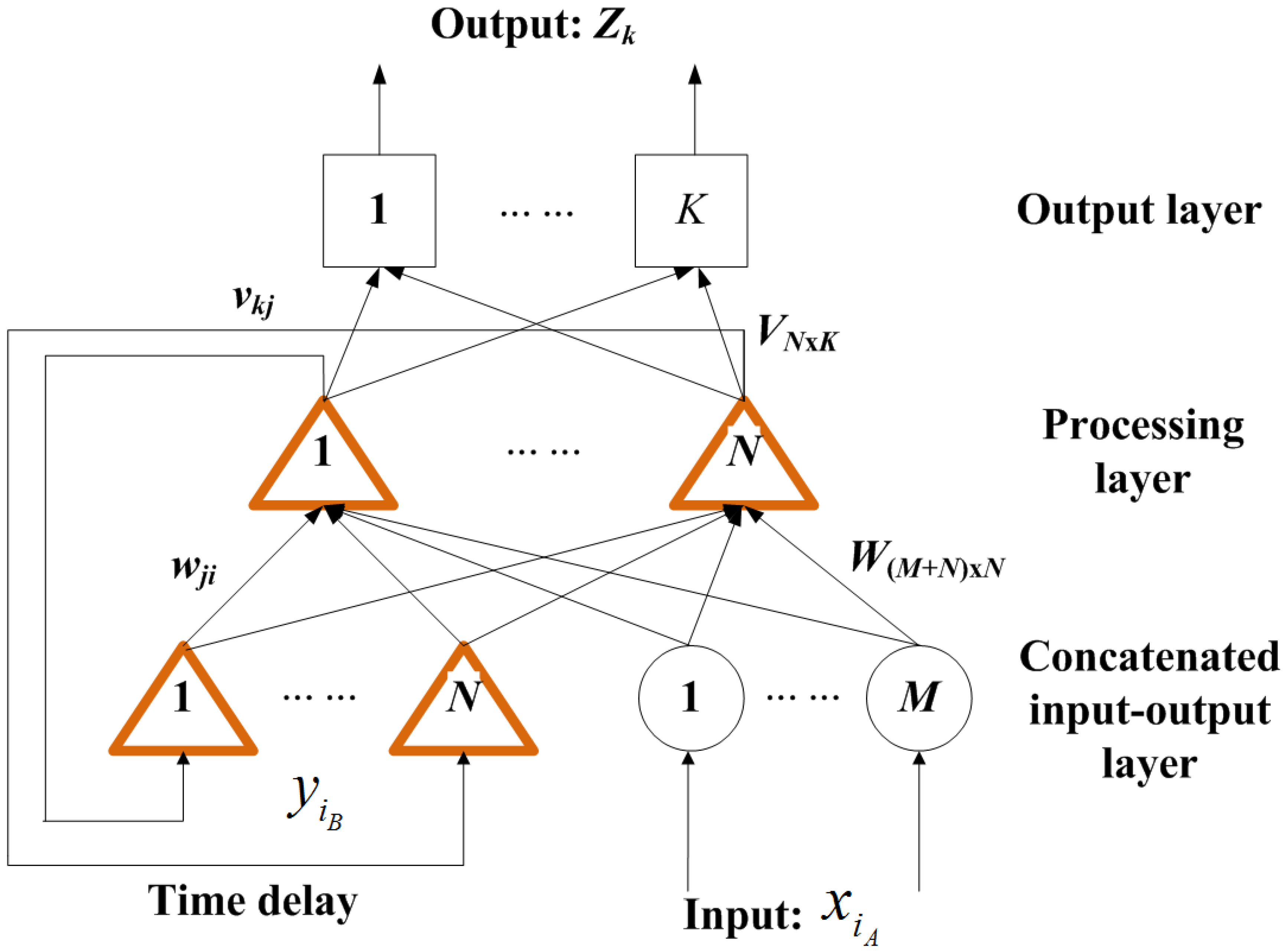
29]. RTRLNN generally contains one or several recurrent loops. The RTRLNN network structure that we adopt in this study is shown in Figure 5. It is a multilayer perceptron and is composed of a concatenated input-output layer, a processing layer, and an output layer. The recurrent loops are recurrent from the output vector of the processing layer to the concatenated input-output layer. Hence, the concatenated input-output layer not only includes the input factor of the outer environment, but also stores the processed information from the processing layer before the current time. This allows the network to establish a temporal mutual connection and a dependent relationship between input variables because of the inner recurrent connection relationship, so the structure and mechanism can effectively learn the connection of the time-series (Elman, 1990 [30]).
Figure 5. Structure of a RTRLNN.
Water 07 06516 g005
The input vector of the concatenated input-output layer contains actual input variables x i A and recurrent input variables y i B ( i A and i B are the number of actual and recurrent inputs, respectively):
u i = [ x i A , y i B ]       f o r i A = 1 , , M i B = 1 , , N
where M and N are the total numbers of actual and recurrent inputs, respectively. The feed-forward propagation of the network first multiplies the input vector ( u i ) with the corresponding weights ( w j i ) to obtain n e t j , then transfers n e t j by a transfer function ( f ( ) ) to obtain the output of the processing layer ( y j ):
n e t j = i i A i B w j i u i
y j = f ( n e t j )
where i, j, and k are the neuron numbers of the concatenated input-output layer, the processing layer, and the output layer, respectively. Multiplying y j with the corresponding weights ( v k j ) and summing them gives n e t k , and transfer n e t k by a transfer function ( f ( ) ) gives the output of the output layer ( z k ):
n e t k = v k j y j
z k = f ( n e t k )
In this study, the feasible transfer functions of the processing layer include tan-sigmoid (expressed in Equation (20)), linear, log-sigmoid, radial basis function, and symmetric saturating linear function, while the output layer is linear. The best suitable transfer function for the forecast model is extracted fully by trail results.
y j = e n e t j e n e t j e n e t j + e n e t j
During RTRLNN training, the network not only continuously executes the message handling, but also revises each connected weighted vector in real-time according to the simulated error that belongs to the learning algorithm. Set d k ( t ) as the target value of neuron k at time t. Then we define a time-varying K × 1 error vector e k ( t ) , whose kth element is:
e k ( t ) = d k ( t ) z k ( t )
Then we define the instantaneous overall network error ( E ( t ) ) at time t as
E ( t ) = 1 2 k = 1 K e k 2 ( t )
The total cost function ( E t o t a l ) is obtained by summing E ( t ) over all time T
E t o t a l = t = 1 T E ( t )
To minimize the cost function, this study applies the recursive steepest gradient descent method and the conjugate gradient algorithm to adjust the weights (V and W) along the negative of Etotal. The other feasible alternative is the Quasi-Newton method which is more time-consuming than the others, so the method is not adopted. Because the total error is the sum of the errors at the individual time-steps, we compute this gradient by accumulating the value of E for each time-step along the trajectory. The weight change for any particular weight ( Δ v k j ( t ) ) can thus be written as
Δ v k j ( t ) = η 1 E ( t ) v k j ( t )
where η1 is the learning-rate parameter. In Equation (24), E ( t ) v k j ( t ) can be written as
E ( t ) v k j ( t ) = e k ( t ) f ( n e t k ( t ) ) y j ( t )
The same method can also be implemented for the specific weight w m n , that is
Δ w m n ( t 1 ) = η 2 E ( t ) w m n ( t 1 )
where η 2 is the learning-rate parameter. The partial derivative E ( t ) w m n ( t 1 ) can be obtained by the chain rule for differentiation as follows:
E ( t ) w m n ( t 1 ) = [ k = 1 K e k ( t ) f ( n e t k ( t ) ) v k j ( t ) ] y j ( t ) w m n ( t 1 )       ( 27 ) y j ( t ) w m n ( t 1 ) = f ( n e t j ( t ) ) n e t j ( t ) w m n ( t 1 )       ( 28 ) n e t j ( t ) w m n ( t 1 ) = i ( i A i B ) ( w j i ( t 1 ) u i ( t 1 ) ) w m n ( t 1 )       ( 29 ) n e t j ( t ) w m n ( t 1 ) = i ( i A i B ) [ w j i ( t 1 ) u i ( t 1 ) w m n ( t 1 ) + w j i ( t 1 ) w m n ( t 1 ) u i ( t 1 ) ]       ( 30 ) s u b j e c t t o w j i ( t 1 ) w m n ( t 1 ) = { 1 , w h e n ( j = m ) ( i = n ) 0 , e l s e       ( 31 )
Equation (30) can be rewritten as
n e t j ( t ) w m n ( t 1 ) = i ( i A i B ) w j i ( t 1 ) u i ( t 1 ) w m n ( t 1 ) + δ m j u n ( t 1 )        ( 32 ) s u b j e c t t o δ m j = { 1 , i f j = m 0 , e l s e        ( 33 )
where δ m j is the Kronecker delta. From the definition of u i ( t ) , we also note that
u i ( t 1 ) w m n ( t 1 ) = { 0 , w h e n i i A y i ( t 1 ) w m n ( t 1 ) , w h e n i i B
According to the propagation mechanism of RTRLNN, the initial state of the network at time t = 0 has no functional dependence on the synaptic weights, that is
y j ( 0 ) w m n ( 0 ) = 0
y j ( t ) w m n ( t 1 ) = f ( n e t j ( t ) ) [ i i B w j i ( t 1 ) y i ( t 1 ) w m n ( t 1 ) + δ m j u n ( t 1 ) ]
Let
y j ( t ) w m n ( t ) = { π m n j ( t ) | ( j i B ) ( m i B ) [ n ( i A i B ) ] } y j ( t ) w m n ( t 1 )
where π m n j ( t ) are the triple indexed sets of variables which describe a dynamic system. For each time step t and all appropriate m, n, and j, the dynamics of the system are governed by
π m n j ( t ) = f ( n e t j ) [ i i B w j i ( t 1 ) π m n i ( t 1 ) + δ m j u n ( t 1 ) ] I . C . : π m n j ( 0 ) = 0
Then the weight changes can be computed as
Δ w m n ( t 1 ) = η 2 [ e k ( t ) f ( n e t k ( t ) ) v k j ( t ) ] π m n j ( t )
Δ v k j ( t ) = η 1 e k ( t ) f ( n e t k ( t ) ) y j ( t )

2.4. Heuristic Construction of ANFIS

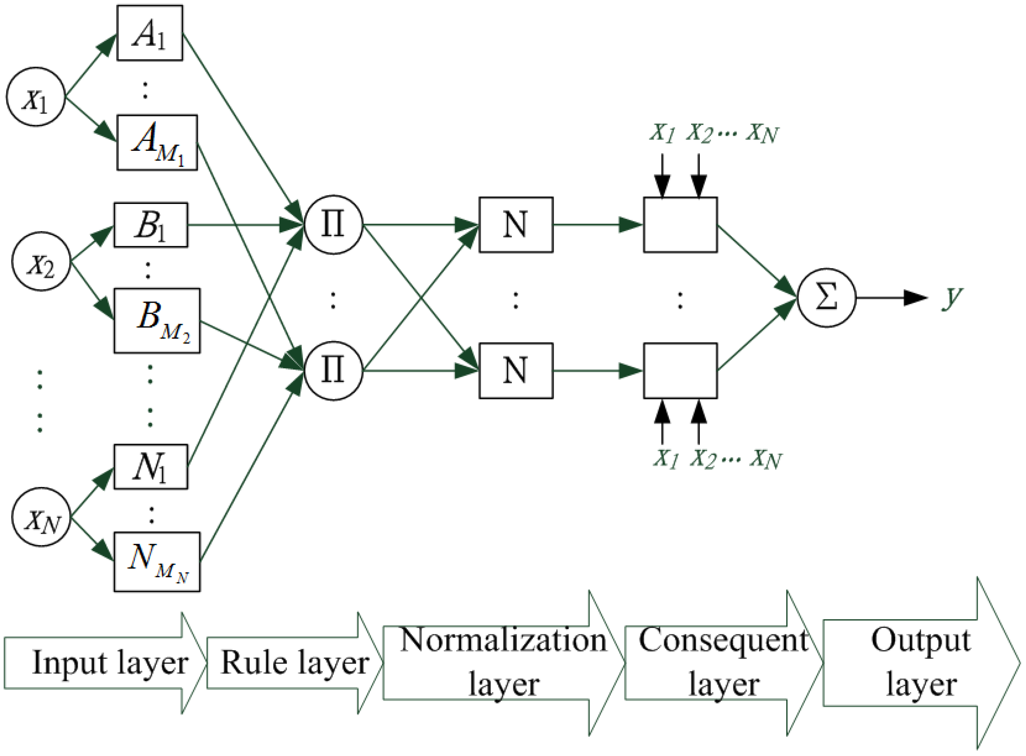
ANFIS was proposed by Jang (1993) [31], and is based on a fuzzy inference system constructed by combining the self-organization characteristics of a neural network. Hence, ANFIS integrates two algorithms to improve its accuracy, and solves for the best parameters by employing capabilities of learning and self-adaption. ANFIS is composed of an input layer, a rule layer, a normalization layer, a consequent layer, and an output layer, as shown in Figure 6. The modeling tool can transform the fuzzy-complex process and phenomenon into an artificial logic language that is therefore a potential approach for typhoon precipitation forecasting. The computation and transmission of each layer is described as follows.
Figure 6. Structure of an ANFIS.
Water 07 06516 g006
(1) Input layer
This layer projects input to a group of fuzzy sets and estimates the values of a group of membership functions. The most common types of membership functions are triangular, trapezoidal, Gaussian, generalized bell-shaped, and sigmoid functions. To retrieve the parameters of the input layer efficiently, this study adopts a group of Gaussian functions as the membership functions with subtractive clustering (SC), which can be expressed as follows:
O 1 , j i = u j i ( x i ) = exp ( x i c j i 2 2 σ j i 2 )      i =1,2, , N    j =1,2, , M i
where u j i ( x i ) is the membership function; cji and σji are the antecedent parameters; N is the number of inputs; and Mi is the number of the fuzzy membership functions of input i.
(2) Rule layer
This layer precedes the antecedent match of the fuzzy logic rule between variables, and then applies a T-norm product operation to obtain the weighted value of each rule, that is,
O 2 , p = w p = i = 1 N u p i ( x i )    p =1, , P
where wp is the weighted value; and P is the number of rules.
(3) Normalization layer
The node of this layer computes the output ratio between the node and all other nodes, that is,
O 3 , p = w ¯ p = w p p = 1 P w p
(4) Consequent layer
The output of the consequent layer node is the product of the outputs of the normalization layer and the Sugeno fuzzy model (Takagi and Sugeno, 1983 [32]), that is,
O 4 , p = w ¯ p f p = w ¯ p ( i = 0 N r p i x i )
where rpi represents the consequent parameters; and x0 is equal to 1.
(5) Output layer
This layer sums the outputs of the previous layer to compute the model output, that is,
O 5 , p = p = 1 P w ¯ p f p = p = 1 P w p f p p = 1 P w p
ANFIS is a feed-forward neural network and is constructed by supervised learning. The network parameters can be divided into antecedent parameters (nonlinear parameters: cji, σji) and consequent parameters (linear parameters: 
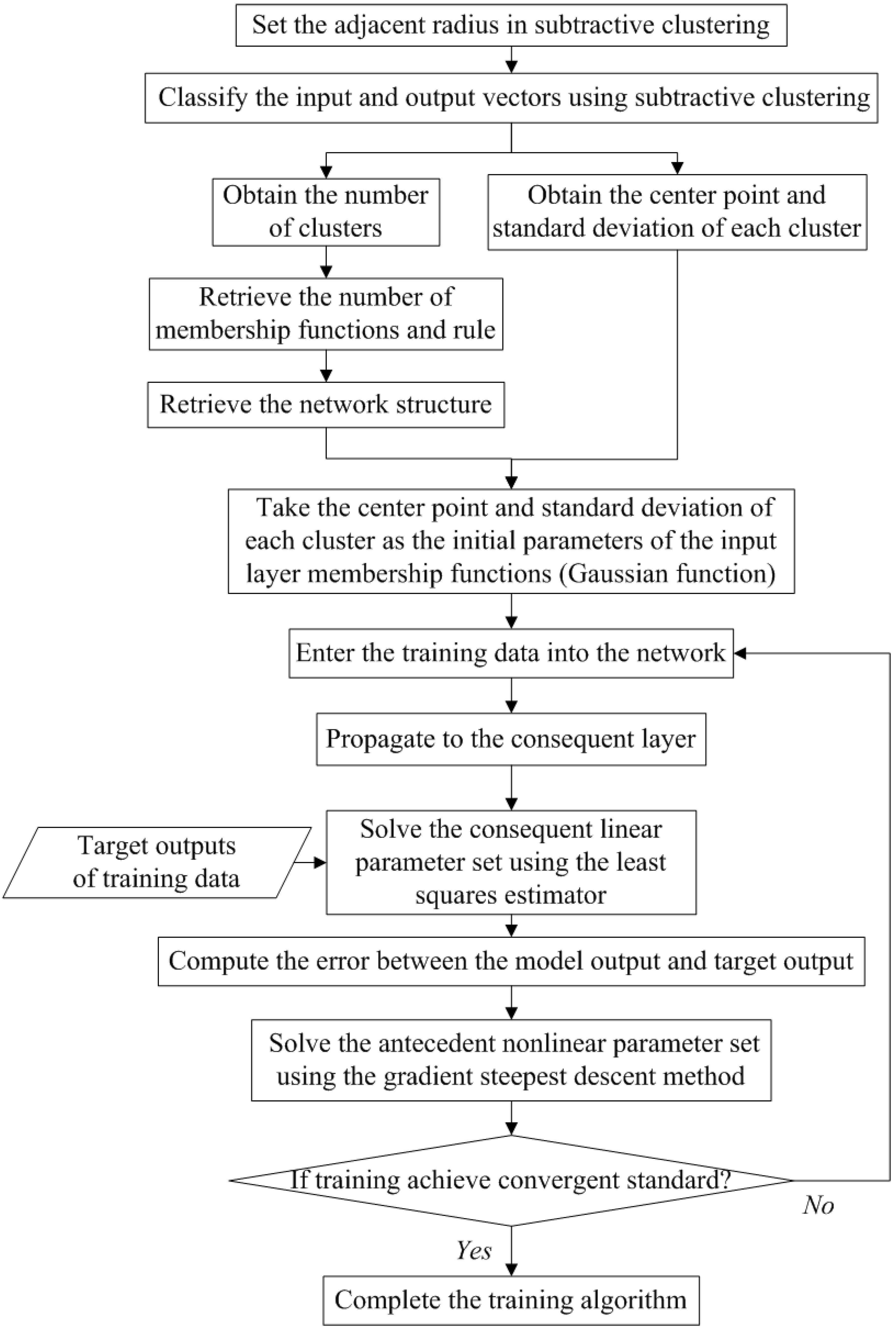
rpi), and the model structure is determined by setting the number of membership functions in the input layer and the number of nodes in the rule layer. The parameters can be solved by the steepest gradient descent method and Newton’s method, for example. However, the methods would be slow and would produce a worse convergence and drop-in local optimum if the searching problem was more complex. To decrease the time for model construction in obtaining the best network structures and parameters, this study constructs ANFIS using hybrid algorithms including subtractive clustering (SC) and a least square estimator (LSE). The input and output vectors were first classified by subtractive clustering before training the model. The number of clusters obtained from the classification was set as the number of membership functions for node fuzzification at the various input layers and the number of nodes at the rule layers. After determining the network structures, the center point and standard deviation of each cluster were taken as the initial parameters of the input layer membership functions (Gaussian function). The training data were then fed into the network with the consequent linear parameter set and the antecedent nonlinear parameter set solved by the least squares estimator and the gradient steepest descent method, respectively. The corresponding algorithm flowchart of the model construction is shown in Figure 7. The network structure significantly reduces the time required to retrieve the optimal number of fuzzy membership functions, number of rules, and network parameters; the optimal network structure and parameters can be obtained after simply setting the adjacent radius in subtractive clustering between 0 and 1 (Jang, 1993 [31]).
Subtractive clustering was employed in the present study to construct fuzzy if-then rules in order to reduce the number of parameters of the fuzzy membership function in the ANFIS model. This was performed to establish a suitable rule base in the fuzzy inference system. Subtractive clustering was proposed by Chiu (1994) [33], in which every data point is treated as the candidate of the cluster center. Subtractive clustering is a fast and independent clustering method: the computational complexity is proportional to the number of data and is independent of the system dimension. For example, x i ( i = 1 , 2 , , n ) are n sets of data in an M-dimensional space and the corresponding density measures D are defined as
D i = j = 1 n exp ( x i x j 2 ( r a / 2 ) 2 )
where the adjacent radius r a is a positive number representing the distance near the center, and the data points outside the radius have minimum impact on the density measure. The density measure is calculated for each data point (xi), and the one with the highest density (Dc1) is selected as the first cluster center (xc1). The definition of the density measure is then modified to select the next cluster center. Setting that xck is the cluster center selected at the kth round, and the corresponding density measure is Dck, the modified formula is as follows:
D i = D i D c k exp ( x i x c k 2 ( r b / 2 ) 2 )
where radius r b has the same definition as r a and is usually set as 1.5 r a so that the selected center will not be too close to that of the previous one. The above procedure of cluster center selection is repeated until a termination condition is reached, or there is a sufficient number of cluster centers.
Figure 7. Flowchart of training the parameter and structure of ANFIS.
Water 07 06516 g007

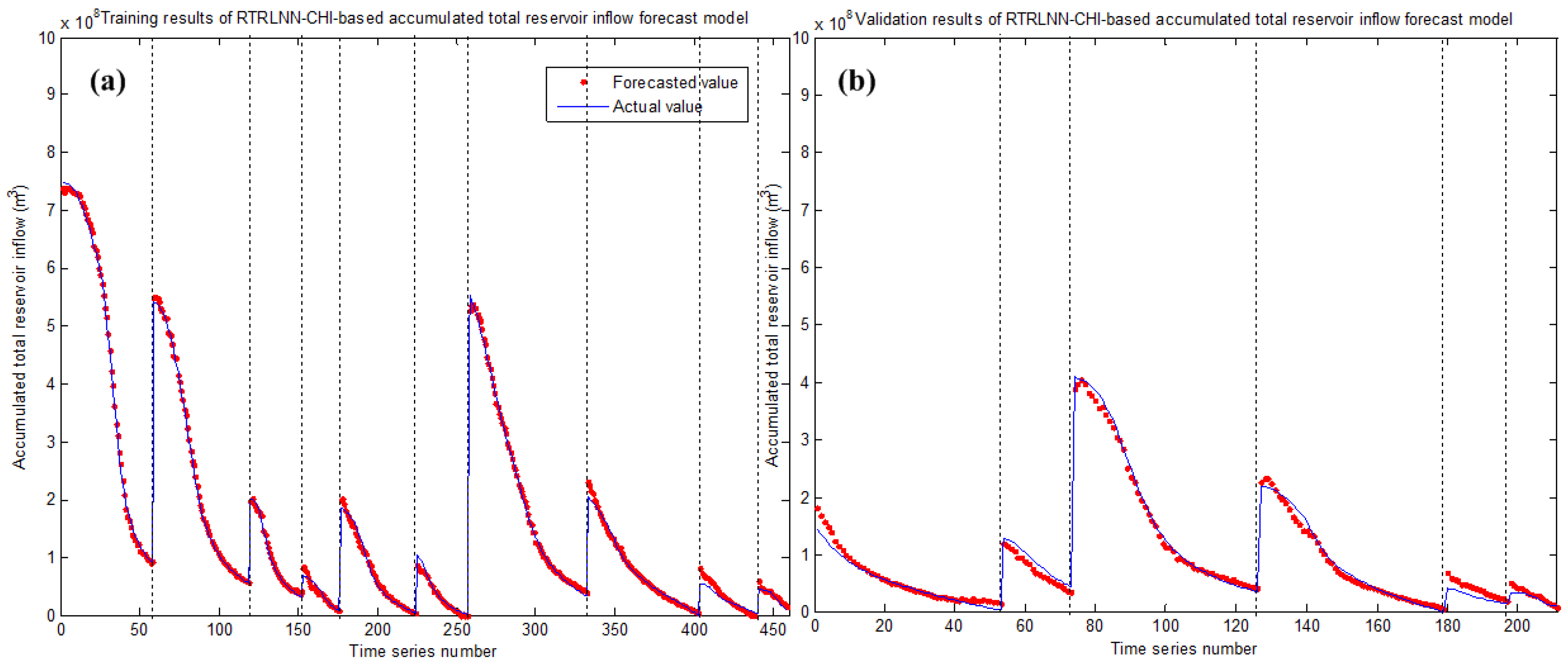
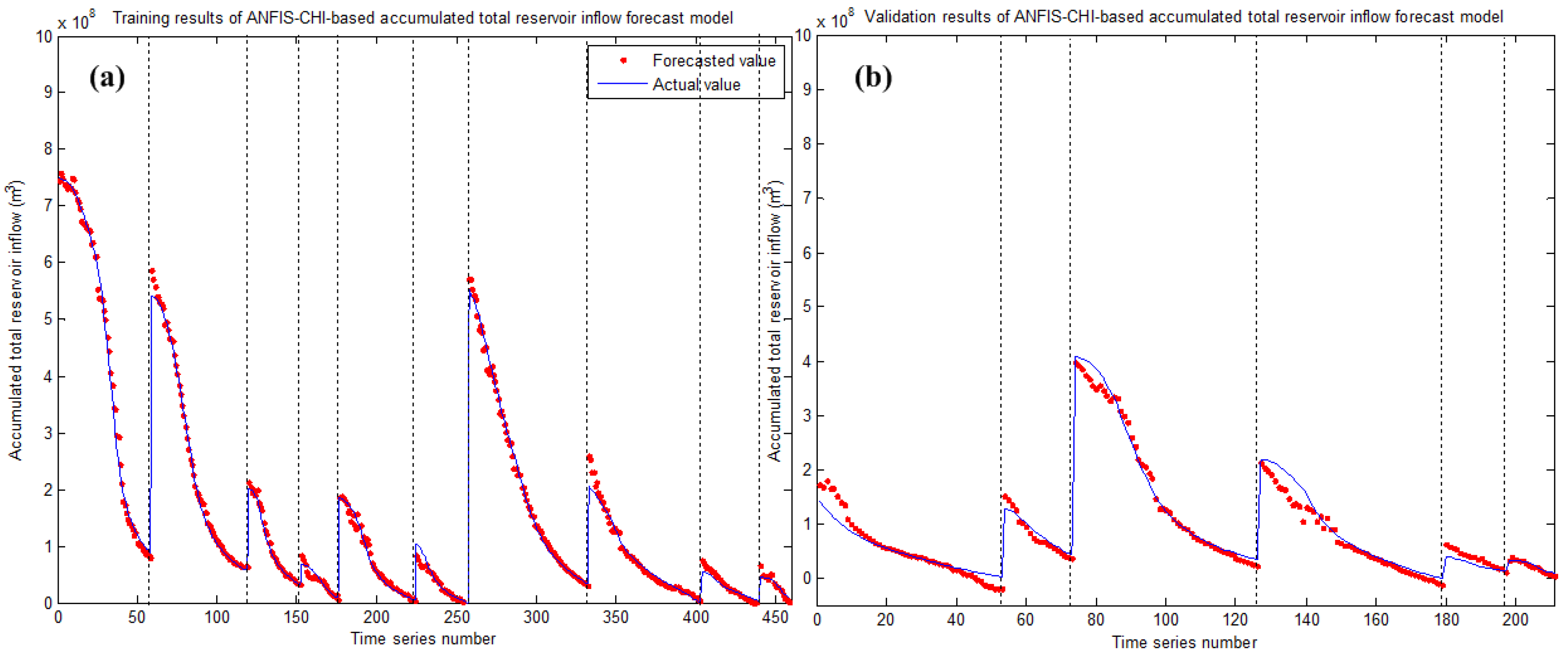
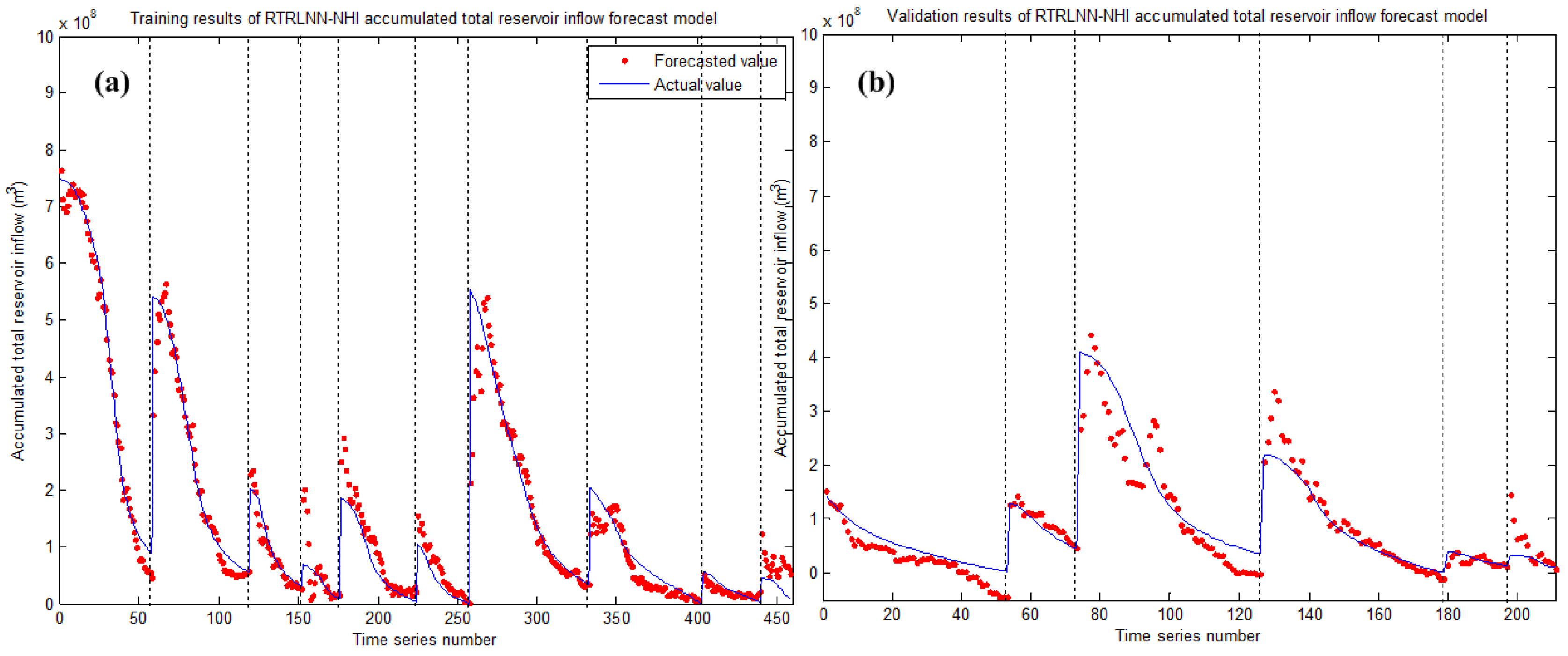
2.5. Analysis of Temporal and Spatial Forecasted Error Feature of the Developed Long Lead-Time Models

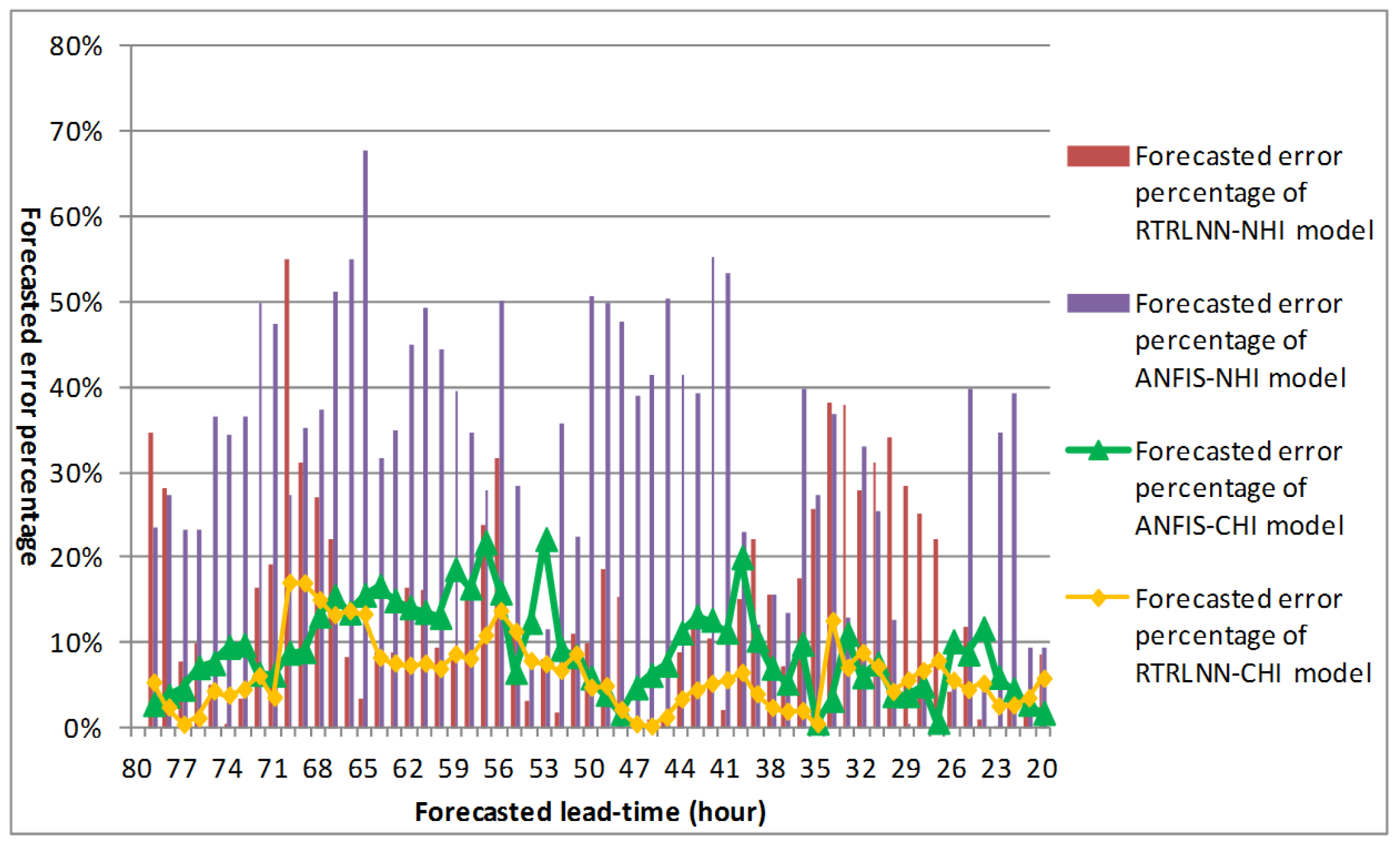
In this research, RTRLNN and ANFIS were used to study four types of coupled heuristic and non-heuristic forecast models (RTRLNN-CHI, RTRLNN-NHI, ANFIS-CHI and ANFIS-NHI) for long lead-time forecast of the total reservoir inflow. To evaluate the forecast accuracy and applicability of the four models on typhoon invasion, analyses were conducted on the characteristics of the temporal and spatial forecast errors for the most optimal forecast case of the four models. Assessments were made as to which model had the best forecast performance. For the analysis of the temporal forecast error, calculations were made for each forecast model for the absolute error between the forecasted time and the forecasted total reservoir inflow during the verification phase of the typhoon event at each field. The errors were then used to assess the capability and limits of the model for the long lead-time forecasting of the total reservoir inflow, which could be calculated as follows:
A E P ( Δ t ) = p = 1 P | Y ^ p ( Δ t ) Y ( Δ t ) p | Y p ( Δ t ) P × 100 %
where A E P ( Δ t ) is average error percentage for forecasted lead-time Δ t , Y ^ p ( Δ t ) and Y ( Δ t ) p are the forecasted and actual accumulated total reservoir inflow on typhoon event number p for forecasted lead-time Δ t , respectively; and P is the total number of typhoon events.
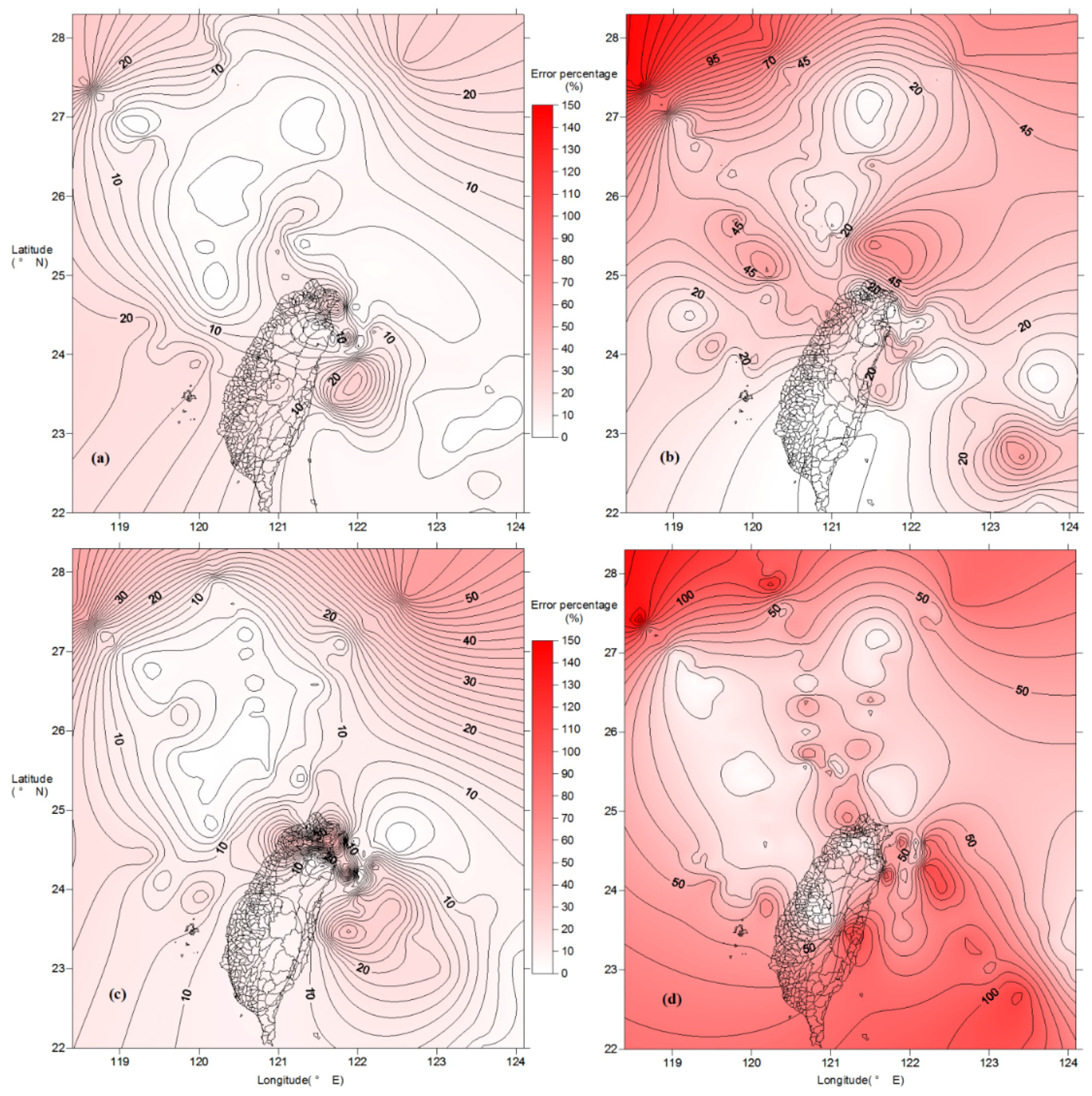
For each forecast model, the analysis of the spatial forecast error included calculation of the absolute error on the forecasted total reservoir inflow at the spatial position of the typhoon center during the verification phase of the typhoon event at each field. These errors were used to discuss the capability and limits of the long lead-time forecasting of the total reservoir inflow for each model when the typhoon center moved to each of the spatial grids, which could be expressed as
A E P ( x , y ) = p = 1 P | Y ^ p ( x , y ) Y ( x , y ) p | Y p ( x , y ) P × 100 %
where A E P ( x , y ) is the average error percentage while the typhoon center is located at longitude x and latitude y, Y ^ p ( x , y ) and Y ( x , y ) p are the forecasted and actual accumulated total reservoir inflow on typhoon event number p while the typhoon center is located at longitude x and latitude y, respectively, and P is the total number of typhoon events.

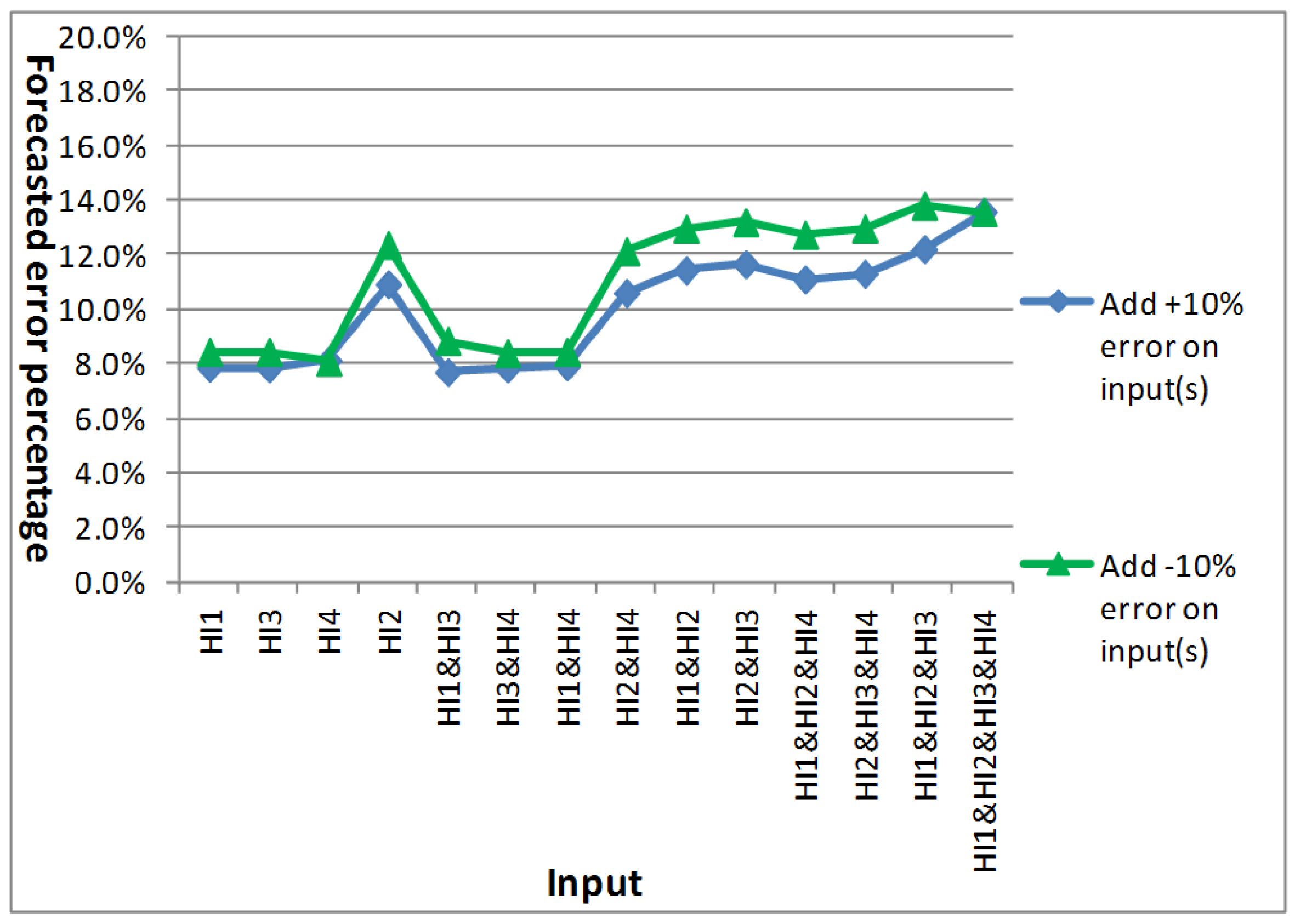
2.6. Output Sensitivity Analysis of Single or Combined Heuristic Inputs Due to Future Forecasted Uncertainty

The coupled heuristic model in this research can forecast the rainfall-runoff hydrology under a specific movement path for the future typhoon, which increases the long lead-time forecast accuracy of the accumulated total reservoir inflow. However, if this model was applied to real-time forecasting, the uncertainty of the meteorology and hydrology for the long lead-time typhoon in the future would be unacceptably high. There would be cases with unavoidable forecast errors on quantities such as the long lead-time total rainfall in the future, the delay from the current time to the maximum rainfall (T0-MP), the delay to the end of the direct runoff (T0-DRE), and the delay to the end of the water retreat in the typhoon event (T0-EE). When such heuristic information is coupled with the input of the heuristic model, it is possible that unexpected errors will be generated on the forecast output of the model. Thus, in order to evaluate the feasibility, applicability, and accuracy of the heuristic model for real-time forecasting, sensitivity analysis was conducted on the effects on the output when forecast errors exist in the heuristic input of the most optimal heuristic model. The above analysis was used to judge whether the forecast accuracy of the heuristic model was better than that of the non-heuristic model for real-time forecasting when errors exist in the input. The expression for the analysis is as shown below:
Y ^ i H ( t ) = f [ R T R L N N C H I A N F I S C H I ] ( x i H ( t ) ± E P x i H ( t ) , X N H ( t ) )
A E P ( i , ± E P ) = t = 1 n | Y ^ i H ( t ) Y ( t ) | Y ( t ) n × 100 %
where Y ^ i H ( t ) is the forecasted value at time t under entering error into heuristic input number i; f [ R T R L N N C H I A N F I S C H I ] is the developed coupled heuristic forecast model; x i H ( t ) is the input value of heuristic input number i at time t; ± E P is the average error percentage based on previous studies; X N H ( t ) is the value of non-heuristic input at time t; Y ( t ) is the actual value at time t; and n is the number of data.

3. Application

3.1. Study Area

The methodology proposed in the present study was applied to the Shihmen Reservoir catchment area, which measures approximately 763.4 km2. The main stream within this area is the Dahan Creek, which is the upper stream of the Tamsui River. The effective capacity is approximately 2.098 × 10⁸ cubic meters. The annual average rainfall in the catchment area is approximately 2350 mm, with 80% of the annual rainfall concentrated in the period between May and October. Most of the rainfall is from typhoon precipitation. The annual inflow of the Shihmen Reservoir is approximately 1.510 billion tons. The study area is shown in Figure 8.

3.2. Data Used in Model Construction

This study used instantaneous observed non-heuristic and coupled heuristic information to forecast accumulated total inflow during current time to the event recessional ending. The output variable was taken as the future accumulated total inflow forecast in the Shihmen Reservoir catchment area. In this study, the end of the typhoon flood event was defined as the moment that simultaneously satisfied the following conditions: (1) the Meteorology Bureau lifted the alarm for typhoon on land and over the sea; (2) rainfall completely stopped in the catchment areas; (3) the reservoir inflow decreased below 300 cms. The model construction included two stages, namely the training and validation stages. The adopted typhoon events for training are Aere, Matsa, Talim, Long-Wang, Wipha, Fung-Wong, Sinlaku, Morakot, Megi, and Meari, and for validation they are Haitang, Sepat, Krosa, Jangmi, and Parma. The total data number for training is 459, and for validation it is 211. The adopted typhoon events for model construction among the training and validation stages are shown in Table 1, and the moving paths of the typhoons used in model construction are shown in Figure 9.
Figure 8. Study area.
Water 07 06516 g008
Table 1. The adopted typhoon events for model construction among the training and validation stages.
Construction StageTyphoon NameTime PeriodTotal Reservoir Inflow (m3)Data NumberTotal Data Number
TrainingAere23–26 August 2004748, 936, 72858459
Matsa4–6 August 2005541, 872, 32461
Talim31 August 2005–2 September 2005201, 308, 58033
Long-Wang2–3 October 200568, 596, 70424
Wipha18–20 September 2007186, 601, 75248
Fung-Wong28–29 July 2008103, 422, 56433
Sinlaku13–16 September 2008554, 322, 60075
Morakot7–10 August 2009205, 435, 98071
Megi21–22 October 201054, 991, 72837
Meari25 June 201144, 826, 01219
ValidationHaitang17–20 July 2005237, 416, 25653211
Sepat18 August 2007128, 935, 22420
Krosa6–8 October 2007409, 855, 82453
Jangmi28–30 September 2008220, 301, 13653
Parma6 October 200940, 997, 34018
Fanapi19 September 201033, 694, 95614
Figure 9. Moving paths of typhoons used in model construction: (a) training; (b) validation.
Water 07 06516 g009

3.3. Results and Discussion

3.3.1. Model Inputs Selection

Correlation analysis was applied in the present study to assess the correlation coefficient between each input factor and the future accumulated total inflow for the Shihmen Reservoir. The selected heuristic model inputs and corresponding correlation coefficients are the future accumulated total basin precipitation (rrank: 0.926), duration from current time to the end of the flood event (rrank: 0.960), duration from current time to the time of DRE (rrank: 0.751), duration from current time to the time of maximum precipitation (rrank: 0.548), and observed-predicted inflow increase/decrease rate (rrank: 0.401). These selected variables are the most correlated inputs among all heuristic candidate predictors and the rrank value of all the selected inputs must be larger than 0.4. Furthermore, the selected non-heuristic model inputs and corresponding correlation coefficients are the observed hourly basin precipitation at the current time (rrank: 0.672), hourly reservoir inflow (rrank: 0.509), typhoon central longitude (rrank: 0.610), central wind speed (rrank: 0.650), and central pressure (rrank: 0.639); these selected variables are the most correlated inputs among all non-heuristic candidate predictors and the rrank values must all be larger than 0.5. Research conducted by Lin and Chen (2005) [34] revealed that excessive model inputs could introduce additional noise into the model, therefore 10 input factors were selected as a maximum based on the correlation coefficients. Based on the above analytical results, the developed heuristic forecast model includes 10 inputs including both heuristic and non-heuristic inputs, and the non-heuristic model only includes five non-heuristic inputs. The heuristic parameters are considered to be essential for use in eliminating the forecasting uncertainty, and for characterizing future long lead-time accumulated total inflow.

3.3.2. Results of Model Construction

In this study, RTRLNN and ANFIS were used to construct coupled heuristic and non-heuristic forecast models for long lead-time forecasting of the future accumulated total inflow for the Shihmen Reservoir. The choice of the particular set of parameters of the optimal model is retrieved by applying an intelligent heuristic searching strategy on the setting structure parameters (i.e., neuron numbers of the processing layer for RTRLNN and the adjacent radius for ANFIS), and the values of the connected parameters corresponding to the setting structure are calibrated by using the heuristic algorithm described in Section 2.3 and Section 2.4. The searching strategy first constructs models by setting a series of neuron numbers (1–15) and adjacent radius (0–1) equally from the feasible domain with the reliable representative amount (10 per neuron number and 100 for adjacent radius), and then the structure parameter of the best model among the equally distributed sampling process was strengthened by construction with more experimental frequency to retrieve the optimal model efficiently. The forecasted outcomes of the most optimal model of the four types of forecast architecture (RTRLNN-CHI, RTRLNN-NHI, ANFIS-CHI, and ANFIS-NHI) are shown in Table 2. The best training and verification results for the RTRLNN-CHI model, ANFIS-CHI model, and RTRLNN-NHI model are shown in Figure 10, Figure 11 and Figure 12, respectively. The MAE values for the verification stage of the RTRLNN-CHI model, RTRLNN-NHI model, ANFIS-CHI model, and ANFIS-NHI model were respectively 11,721,556 m3, 30,475,270 m3, 14,429,374 m3, and 53,236,429 m3, while the CC values for the verification were 0.979, 0.876, 0.975, and 0.658, respectively. The results indicate that the respective forecast accuracy and stability of the RTRLNN-CHI and ANFIS-CHI models are significantly higher than those of the RTRLNN-NHI and ANFIS-NHI models. This shows that the proposed heuristic forecast model may be highly accurate in its forecast of the total reservoir inflow under the following conditions: (1) when the input includes key inputs such as the future accumulated total precipitation and the delays from the current moment to the key hydrology points of the hydrograph (maximum precipitation, direct runoff ending, and event recessional ending); (2) with assistance of the comprehensive simulation of the real-time observed atmospheric factors and rainfall-runoff factors of the typhoon.
Table 2. Best assessment indexes values of the four kinds of constructed models.
Structure Parameters/Assessment IndexesRTRLNN-CHI ModelRTRLNN-NHI ModelStructure Parameters/Assessment IndexesANFIS-CHI ModelANFIS-NHI Model
Best node number of hidden layer39Best adjacent radius/rule number0.922/20.836/3
MAE of training (m3)458745922430139MAE of training (m3)724916059066261
MAE of validation (m3)1172155630475271MAE of validation (m3)1442937553236429
CC of training0.9990.980CC of training0.9980.867
CC of validation0.9800.876CC of validation0.9760.659
The input information for the RTRLNN-NHI and ANFIS-NHI models only included the current real-time observed conditions of the typhoon atmosphere and rainfall-runoff status. The average forecasted accuracy of the RTRLNN-NHI and ANFIS-NHI models is respectively worse than that of the RTRLNN-CHI/ANFIS-CHI models by 1.6/1.11 times and 3.54/2.68 times, and average forecasted stability is worse by 10.5%/10.2% and 32.8%/32.5%. Hence, these two non-heuristic models could not be used to accurately and physically simulate the accumulated total reservoir inflow after long lead-time changes in the meteorology and hydrology. The reason is that the model inputs only have initial conditions (observed rainfall-runoff variables) but do not have boundary conditions for future periods to simulate the shape and duration of future inflow hydrographs. This obviously caused the forecasting accuracy and stability of the accumulated total inflow at the moment of maximum rainfall in the early stage of the event to be inferior to that at the later stages after the flood peaked. Moreover, the activation function in the hidden layer of the most optimal RTRLNN-based forecast model for the total reservoir inflow was a tan-sigmoid transfer function, while the activation function in the output layer was a linear activation function. The reason is that the shape of the tan-sigmoid function is similar to the cumulative distribution function (CDF) of the inflow hydrograph, and the shape of the CDF is exactly the inverse of the accumulated total inflow hydrograph. Hence, the tan-sigmoid function can simulate future accumulated total inflow better than the other shapes of functions. Furthermore, the numbers of neurons for the processing layer of the most optimal models in the RTRLNN-CHI and RTRLNN-NHI models were three and nine, respectively, and the rule numbers for the most optimal ANFIS-CHI and ANFIS-NHI models were two and three, respectively. This indicates that there was insufficient input information to represent future boundary conditions of the typhoon rainfall-runoff relationship over a long lead-time in the non-heuristic model. Therefore, a more complicated and time-consuming model is required to simulate the accumulated total reservoir inflow in the future.
In addition, from the evaluation-index point of view, for the two heuristic models, the overall forecast accuracy and stability of the RTRLNN-CHI model for forecasting the total reservoir inflow was slightly better than that of the ANFIS-CHI model by 0.23 times of MAE and 0.41% of CC. The reason is that there is a fixed-ratio real-time feedback calculation mechanism in the structure of the RTRLNN model. When the simulation mechanism and characteristics of the model were applied to forecasting time-varying output targets with a long lead-time and high uncertainty, better forecasting results were obtained than with the ANFIS model, which lacks flexibility in the input and rule layers that were used.
Figure 10. Training and validation results of RTRLNN-CHI-based accumulated total reservoir inflow forecast model: (a) training stage; (b) validation stage.
Water 07 06516 g010
Figure 11. Training and validation results of ANFIS-CHI-based accumulated total reservoir inflow forecast model: (a) training stage; (b) validation stage.
Water 07 06516 g011
Figure 12. Training and validation results of RTRLNN-NHI-based accumulated total reservoir inflow forecast model: (a) training stage; (b) validation stage.
Water 07 06516 g012

3.3.3. Analytical Results of Temporal and Spatial Forecasted Error Feature of the Developed Models

In this research, characteristic analyses were made on the temporal and spatial forecast errors of the four forecast models (RTRLNN-CHI, RTRLNN-NHI, ANFIS-CHI, and ANFIS-NHI) for long lead-time and total reservoir inflow. The analysis targets were six typhoon events for verification, which were used to evaluate the limits and applicability of the four models for long lead-time forecasting. Judgments were also made on the range of the typhoon center where the future total reservoir inflow may be accurately and appropriately forecasted. The average error percentages of the four developed accumulated total inflow forecast models across long lead-times are shown in Table 3, and a comparison of the temporal forecasted error features of the developed models across long lead-times is given in Figure 13. The percentages of the average forecast errors in the forecast time range of 24 to 48 h for the four models (RTRLNN-CHI, RTRLNN-NHI, ANFIS-CHI, and ANFIS-NHI), ( Δ t = 24 48 A E P ( Δ t ) 24 ), were 4.6%, 16.7%, 7.7%, and 27.1%, respectively. The average error percentages (AEP) for the period of 48 to 72 h, ( Δ t = 48 72 A E P ( Δ t ) 24 ), were 9.3%, 16.1%, 12.1%, and 39.3%, respectively. The AEP in the period of 20 to 79 h, ( Δ t = 20 79 A E P ( Δ t ) 60 ), were 6.3%, 15.2%, 9.2%, and 31.8%, respectively. The results indicate that the long lead-time forecast accuracy of the heuristic model is obviously better than that of the non-heuristic model by 9%–23% for a lead-time of 24–48 h and 4%–30% for a lead-time of 48–72 h. The forecast error of the heuristic model did not significantly increase along with the increasing of the forecasted lead-time. The hydrograph patterns of the reservoir inflow for the meteorology and hydrology of the future typhoon can be appropriately simulated ahead of time with heuristic inputs. Therefore, the accumulated total inflow can be accurately forecasted for the long lead-time future. Furthermore, there was a highly complicated nonlinear relationship between the rainfall from the typhoon meteorology and the runoff in the catchment area from hydrology. There was better flexibility in the calculation mechanism of the RTRLNN model than in the ANFIS model. RTRLNN had detailed linkage between various types of inputs and outputs. It also calculated feedback information in real-time. Moreover, the accuracies of the various forecasted time intervals using the RTRLNN-CHI model were better than those obtained using the ANFIS-CHI model. The forecast error was less than 10% when the forecasted lead-time reached three days. The AEP for a forecasted lead-time of an average 49 h, ( Δ t = 20 79 A E P ( Δ t ) 60 ), was only 6.3% for the RTRLNN-CHI model. Hence, a long lead-time forecast model for the accumulated total reservoir inflow was successfully developed using the heuristic technique in this study.
Table 3. Average error percentage of the four developed models across long lead-times.
Forecasted Lead-TimeRTRLNN-CHI ModelRTRLNN-NHI ModelANFIS-CHI ModelANFIS-NHI Model
During 24 to 48 h4.6%16.7%7.7%27.1%
During 48 to 72 h9.3%16.1%12.1%39.3%
During 20 to 79 h6.3%15.2%9.2%31.8%
Figure 13. Comparison of temporal forecasted error features of the four developed accumulated total inflow forecast models across long lead-times.
Water 07 06516 g013
The comparison of the spatial forecasted error feature of the four developed accumulated total inflow forecast models for the Shihmen Reservoir with relation to the central location of the typhoon is shown in Figure 14. This figure represents the absolute error percentage ( A E P ( x , y ) ) on the forecasted total reservoir inflow in the catchment area of the Shihmen Reservoir when the typhoon center was moving in the vicinity of any region in Taiwan (in the range of longitude 118–124 degrees, latitude 22–28 degrees). It can be seen from the spatial distributions of the forecast errors of the four models that the overall error space and range of the heuristic models (e.g., Figure 14a for the RTRLNN-CHI model, and Figure 14c for the ANFIS-CHI model) are much smaller than those of the non-heuristic models (e.g., Figure 14b for the RTRLNN-NHI model, and Figure 14d for the ANFIS-NHI model). In the error spatial distribution map of the RTRLNN-CHI model, the range where the A E P ( x , y ) was less than 10% (which was about 61% of the researched range) was much bigger than that of the ANFIS-CHI model (which was about 47% of the researched range). The range where the A E P ( x , y ) was greater than 20% (which was about 13% of the researched range) was much smaller than that of the ANFIS-CHI model (which was about 32% of the researched range). Figure 14 confirms that the forecast accuracy and stability of the RTRLNN-CHI model were better than those of other models when typhoon invasion was at the basin of the Shihmen Reservoir. When the typhoon center was in the southeast of Taiwan, the structure and meteorology field after the typhoon passed Taiwan was destroyed by the terrain. There was also the co-existing effects of the monsoon. Therefore, there was a significant difference between the future typhoon meteorology and rainfall-runoff conditions and the observed data when the typhoon center was in the southeast of Taiwan. As a result, the forecast error on the total reservoir inflow of the typhoon when it is located in the southeast of Taiwan is greater than that when the typhoon center is located elsewhere. However, after the typhoon center passed Taiwan, the circulation structure was not affected by the terrain. Hence, the forecast error on the total reservoir inflow was relatively small.

3.3.4. Sensitivity Analysis Results of Output with Relation to Heuristic Inputs Due to Future Forecasted Uncertainty

In order to evaluate the feasibility, applicability, and accuracy of the heuristic model when applied to real-time forecasting, a sensitivity analysis was conducted on the forecasted error effects of the outputs with relation to single or combined heuristic inputs for the most optimal heuristic model (RTRLNN-CHI). According to the previously developed short lead-time hydrological forecast models [35,36], an average forecast error ( ± E P ) of 10% was assumed on each heuristic input, which was inputted into the model to simulate the absolute error percentage ( A E P ( i , ± E P ) ) of the forecast. The results from the analysis are shown in Figure 15, where Heuristic input 1 (HI1) is the future accumulated total precipitation, HI2 is the duration from the current time to the flood recessional ending time, HI3 is the duration from the current time to the DRE time, and HI4 is the duration from the current time to the maximum precipitation time. The results displayed show that when ±10% error was inputted with HI2, the maximum output error would appear regardless of whether the case was that of a single input or combinations of multiple inputs. This indicates that the flood duration is the most important factor in forecasting the future accumulated total reservoir inflow, which is also the most sensitive input for the output of the model. Among all the combinations of heuristic input errors, the average forecast error was 9.98% for a 10% overestimation on the input, with a maximum of 13.6% (when there are 10% errors on all of HI1, HI2, HI3, and HI4). For the case of underestimation with a 10% error on the input, the average forecast error was 11.01%, with a maximum of 13.6%. There was an additional 1.03% error on the output for the 10% underestimation error on the heuristic inputs when compared to the case of 10% overestimation on the input. These results indicate that the absolute error percentage (13.6%) of the heuristic model with a 10% error on all the heuristic inputs was still lower than that of the most optimal non-heuristic model (RTRLNN-NHI), A E P = 15.2%. This shows that the real-time forecast accuracy of the RTRLNN-CHI model is still better than that of the non-heuristic models (RTRLNN-NHI and ANFIS-NHI) even when there are errors on the heuristic inputs.
Figure 14. Comparison of spatial forecasted error feature of the four developed accumulated total inflow forecast models for the Shihmen Reservoir with relation to the typhoon central location: (a) RTRLNN-CHI model; (b) RTRLNN-NHI model; (c) ANFIS-CHI model; and (d) ANFIS-NHI model.
Water 07 06516 g014
Figure 15. Sensitivity analysis results of model output with relation to single or combined heuristic inputs due to future forecasted uncertainty.
Water 07 06516 g015

3.3.5. Construction Results of Heuristic Forecast Database for Heuristic Inputs

In this study, heuristic data mining techniques were used to construct a forecast database for the relationship between the position of the typhoon center, the rainfall hyetograph, and the inflow hydrograph in the catchment area from historical samples. The database was constructed to facilitate forecasting of the future accumulated total precipitation. Similarly, heuristic data mining techniques can also be applied on the delay of the future typhoon invasion by constructing a forecast database from relationships on the spatial position distribution of the typhoon center when the water has completely retreated, the moment of maximum rainfall, and the end time of direct runoff in historical samples. The characteristic map of the typhoon center position vs. the rainfall in the Shihmen Reservoir basin is as shown in Figure 16, which is the contour map after Kriging interpolation of the spatial sample information (X axis (typhoon central longitude), Y axis (typhoon central latitude), Z axis (basin precipitation of Shihmen Reservoir)). In this figure, strong rainfalls occurred when the typhoon center was at the southeast of Taiwan because the typhoon was under the influence of the Coriolis Effect. The air exhibits counterclockwise rotation in the Northern Hemisphere. When the typhoon was in the southeast of Taiwan, the typhoon rain belt entrained by the wind field under counterclockwise rotation was not blocked by the terrain of the mostly flat lands before entering the catchment area of the Shihmen Reservoir. After the rain belt entered the catchment area of the Shihmen Reservoir from the northwest to the southeast, it was blocked by the Snow-Capped mountain range. The catchment area of the Shihmen Reservoir belonged to the upwind side and heavy rain would happen then. In contrast, when the typhoon was not in the southeast of Taiwan, the rain belt entrained by the wind field was blocked by the Snow-Capped mountain range, the Central mountain range, and the Yusan mountain range before entering the catchment area of the Shihmen Reservoir. The catchment area of the Shihmen Reservoir was at leeward and there were no heavy rains in the Shihmen Reservoir at this time. With the assistance of this figure, the rainfall hyetograph in the catchment area of the Shihmen Reservoir during the future whole typhoon flood event can be obtained from the combined information of the hourly forecasted positions of the future typhoon center, the real-time estimated amount of rainfall, and the correction from the observed amount. The desired forecast of the total rainfall for the total reservoir inflow was obtained by summing over the rainfall hyetograph.
In this study, derivations on the spatial characteristics of the position distribution of the typhoon center were made for the moment when the maximum rainfall occurred, the direct runoff ended, and the water retreat ended in the typhoon flood events. First, the basin of the Shihmen Reservoir was located as the ellipse Eb in Figure 16, and then the terrain factors that might affect the rainfall in the reservoir basin were identified. Then, an axis (Line M1–M2) was marked along the direction of the Snow-Capped mountain range. The second axis (Line P1–P2), was defined as being perpendicular to Line M1–M2. Using these two axes as the reference, a contour map was created of the spatial distribution of the positions of the typhoon center when the water retreated below 300 cm of the reservoir inflow for the periods when a typhoon alarm is historically issued on land until the alarm is lifted. This resulted in the elliptical distribution line (EE), from which the starting time of the forecast and the ending time of the water retreat could be determined. Regarding the model construction event, a contour map could be made for the spatial distribution of the positions of the typhoon center between the start of the rainfall and the end of the direct runoff for historical typhoon flood events. This resulted in the elliptical distribution line EDRE. Further, the elliptical distribution line EMP could be obtained from the contour map of the spatial distribution of the typhoon center when the maximum rainfall occurred in the historical typhoon flood events. The time of the maximum rainfall may be determined from this distribution line (EMP) and the contour lines of rainfall.
Figure 16. Construction results of heuristic forecast database for the Shihmen basin precipitation and duration characteristics curves with relation to the typhoon central location.
Water 07 06516 g016
In Figure 16, the distribution lines were mainly elliptical, which was due to the Coriolis effect and the Terrain effect during the movements of the typhoon. When the path and direction of typhoon movement and the spatial distribution of terrain height are non-uniform, the distribution lines are elliptical instead of circular. The main axis of the ellipse was related to the direction of the terrains and mountains, so the elliptical distribution was a rotation of the main axis. Besides, the delay of the hydrograph pattern of rainfall was mainly dominated by the moving path of the typhoon. Because the Coriolis effect acted on the typhoon, it moved toward the direction of 270° to 360°, while the synthetic moving direction coincided with Line P1–P2, i.e., the perpendicular line of the Snow-Capped mountain range. Therefore, the long axes of EE and EDRE are along Line P1–P2, while the long axis of EMP was in the direction of the Snow-Capped mountain range (Line M1–M2) because whether or not strong rainfall occurred was mainly related to the angle and position between the direction from which the rain belt of typhoon entered the reservoir basin and the direction of the Snow-Capped mountain range. In addition, from a monsoon climatology point of view, Taiwan is mainly affected by southwest monsoons from mid-March to mid-September, and is predominantly under the effects of the northeast monsoon at other times. When the typhoon center was located in quadrants I and II in Figure 16, the wind field with counterclockwise rotation easily accompanied the northeast monsoon in the basin direction of the Shihmen Reservoir; when it was located in quadrants III and IV, the wind field was easily accompanied by the southwest monsoon. For typhoon invasion in quadrants I and II after mid-September and in quadrants III and IV during mid-March and mid-September, the typhoon was easily accompanied by co-existing effects of the monsoon to increase rainfall duration and precipitation. The contour lines of EE, EDRE, and EMP can be expressed with the following equations:
[ ( x cos 49 ° + y sin 49 ° ) Δ d l o n . 13481.3 (E,km) ] 2 [ 1113.92  (km) ] 2 + [ ( x sin 49 ° + y cos 49 ° ) Δ d l a t . 2758.7 (N,km) ] 2 [ 1179.209  (km) ] 2 = 1
[ ( x cos 49 ° + y sin 49 ° ) Δ d l o n . 13481.3 (E,km) ] 2 [ 885.2  (km) ] 2 + [ ( x sin 49 ° + y cos 49 ° ) Δ d l a t . 2758.7 (N,km) ] 2 [ 942.7  (km) ] 2 = 1
[ ( x cos 49 ° + y sin 49 ° ) Δ d l o n . 13481.3 (E,km) ] 2 [ 587.4  (km) ] 2 + [ ( x sin 49 ° + y cos 49 ° ) Δ d l a t . 2758.7 (N,km) ] 2 [ 425.6  (km) ] 2 = 1
where Δ d l o n . and Δ d l a t . are the representative distance of each longitude and latitude, respectively.

4. Conclusions

Typhoon long lead-time rainfall-runoff is characterized as a chaotic, fuzzy, highly uncertain, and nonlinear system. The routing mechanism and characteristics of the real-time recurrent learning neural network (RTRLNN) and the adaptive network-based fuzzy inference system (ANFIS) have the potential ability to reason and learn using deterministic real-time recurrent routing and fuzzy logic. Therefore, the present study applied RTRLNN and ANFIS combined with multiple artificial intelligence-based heuristic techniques to develop coupled heuristic long lead-time accumulated total reservoir inflow forecast models (RTRLNN-CHI and ANFIS-CHI), in order to improve the accuracy and stability of long-term accumulated total inflow forecasting. The proposed system was evaluated by a comparison with the RTRLNN- and ANFIS-based non-heuristic models (RTRLNN-NHI and ANFIS-NHI). The inputs of the heuristic models are composed of coupled observed non-heuristic inputs (typhoon characteristics factors, hourly basin precipitation, hourly reservoir inflow) and forecasted heuristic inputs (future accumulated total precipitation, duration from the current time to the time of maximum precipitation, direct runoff ending and event recessional ending, and observed-predicted inflow increase/decrease rate). The present study first employed non-parametric correlation analysis to assess the most appropriate input variables for long lead-time non-heuristic and heuristic models. This study also analyzed temporal and spatial forecasted error features to assess the goodness and applicability of the developed four long lead-time models, and we also analyzed the output sensitivity of single or combined heuristic inputs to determine whether the developed heuristic model can suffer the impact of future forecasted uncertainty and error on inputs.
The proposed method was applied to Taiwan’s Shihmen Reservoir catchment area with a study period from 2004 to 2012. The results showed lead us to the following conclusions. (1) The accuracy and stability of the RTRLNN-based long lead-time accumulated total reservoir inflow prediction model are better than that of the ANFIS-based model. This is because RTRLNN incorporates a real-time recurrent deterministic routing mechanism with a more elastic and fine connection than ANFIS. (2) Under the synthesized simulation using key heuristic inputs of future total precipitation, flooding duration, and OPIID rate with other real-time observed hydrometeorological factors, the coupled heuristic RTRLNN-based model (RTRLNN-CHI, average error percentage (AEP): 6.3%, average forecasted lead-time: 49 h) and ANFIS-based model (ANFIS-CHI, AEP: 9.2%) could achieve a better prediction than the non-heuristic model (RTRLNN-NHI, AEP: 15.2%; ANFIS-NHI, AEP: 31.8%) because of the full consideration of different runoff/infiltration scenarios and initial/boundary conditions in each time step. (3) The hydrograph pattern of the reservoir inflow for the future typhoon meteorology and hydrology could be appropriately simulated ahead of time by using heuristic inputs. The accuracy of the long lead-time (24–72 h) total inflow forecast at the typhoon center during the invasion period in Taiwan (longitude 118–124 degrees, latitude 22–28 degrees) of the heuristic model was obviously better than that of the non-heuristic model. (4) When there were 10% errors on all the heuristic inputs, the AEP (13.6%) of the heuristic model was still lower than that of the most optimal non-heuristic model (RTRLNN-NHI, 15.2%). This indicates that the real-time forecast accuracy of the RTRLNN-CHI model even with errors on the heuristic inputs is still higher than that of the non-heuristic models (RTRLNN-NHI and ANFIS-NHI).
The key factors to effectively forecast long lead-time accumulated total reservoir inflow under a complex typhoon effect in real-time rely on the predicted accuracy of the meteorological-hydrological heuristic inputs and the associated data-preprocessing process. Future study can focus on improving the predicted accuracy of the heuristic inputs by coupling with novel numerical weather forecast models as a basis to provide future rainfall-runoff boundary conditions for a soft-computing model.

Acknowledgments

This research was partially supported by the Ministry of Science and Technology, Taiwan (Grant Nos. MOST103-2221-E-002-246 and MOST104-2111-M-464-001). In addition, the authors are indebted to the reviewers for their valuable comments and suggestions.

Author Contributions

Chien-Lin Huang performed the model construction and experiments, analyzed the data and wrote the paper; Nien-Sheng Hsu and Chih-Chiang Wei conceived and designed the models and experiments.

Conflicts of Interest

The authors declare no conflict of interest. The founding sponsors had no role in the design of the study; in the collection, analyses, or interpretation of data; in the writing of the manuscript, and in the decision to publish the results.

References

  1. Lin, G.F.; Chen, G.R.; Huang, P.Y.; Chou, Y.C. Support vector machine-based models for hourly reservoir inflow forecasting during typhoon-warning periods. J. Hydrol. 2009, 372, 17–29. [Google Scholar] [CrossRef]
  2. Lin, G.F.; Wu, M.C.; Chen, G.R.; Tsai, F.Y. An RBF-based model with an information processor for forecasting hourly reservoir inflow during typhoons. Hydrol. Process. 2009, 23, 3598–3609. [Google Scholar] [CrossRef]
  3. Hsu, N.S.; Huang, C.L.; Wei, C.C. Real-time forecast of reservoir inflow hydrographs incorporating terrain and monsoon effects during typhoon invasion by novel intelligent numerical-statistic impulse techniques. J. Hydrol. Eng. 2015, 20. [Google Scholar] [CrossRef]
  4. Webster, P.J.; Holland, G.J.; Curry, J.A.; Chang, H.R. Changes in tropical cyclone number, duration, and intensity in a warming environment. Science 2005, 309, 1844–1846. [Google Scholar] [CrossRef] [PubMed]
  5. Wu, L.; Wang, B.; Geng, S. Growing typhoon influence on East Asia. Geophys. Res. Lett. 2005, 32. [Google Scholar] [CrossRef]
  6. Knutson, T.R.; McBride, J.L.; Chan, J.; Emanuel, K.; Holland, G.; Landsea, C.; Held, I.; Kossin, J.P.; Srivastava, A.K.; Sugi, M. Tropical cyclones and climate change. Nat. Geosci. 2010, 3, 157–163. [Google Scholar] [CrossRef] [Green Version]
  7. Bertoni, J.C.; Tucci, C.E.; Clarke, R.T. Rainfall-based real-time flood forecasting. J. Hydrol. 1992, 131, 313–339. [Google Scholar] [CrossRef]
  8. Lardet, P.; Obled, C. Real-time flood forecasting using a stochastic rainfall generator. J. Hydrol. 1994, 162, 391–408. [Google Scholar] [CrossRef]
  9. Toth, E.; Brath, A.; Montanari, A. Comparison of short-term rainfall prediction models for real-time flood forecasting. J. Hydrol. 2000, 239, 132–147. [Google Scholar] [CrossRef]
  10. Anderson, M.; Chen, Z.; Kavvas, M.; Feldman, A. Coupling HEC-HMS with atmospheric models for prediction of watershed runoff. J. Hydrol. Engine 2002, 7, 312–318. [Google Scholar] [CrossRef]
  11. Collischonn, W.; Haas, R.; Andreolli, I.; Tucci, C.E.M. Forecasting river uruguay flow using rainfall forecasts from a regional weather-prediction model. J. Hydrol. 2005, 305, 87–98. [Google Scholar] [CrossRef]
  12. Dahlke, H.E.; Easton, Z.M.; Fuka, D.R.; Walter, M.T.; Steenhuis, T.S. Real-time forecast of hydrologically sensitive areas in the salmon creek watershed, New York state, using an online prediction tool. Water 2013, 5, 917–944. [Google Scholar] [CrossRef]
  13. Brath, A.; Montanari, A.; Toth, E. Neural networks and non-parametric methods for improving real-time flood forecasting through conceptual hydrological models. Hydrol. Earth Syst. Sci. 2002, 6, 627–639. [Google Scholar] [CrossRef]
  14. Hsu, N.S.; Wei, C.C. A multipurpose reservoir real-time operation model for flood control during typhoon invasion. J. Hydrol. 2007, 336, 282–293. [Google Scholar] [CrossRef]
  15. Kitanidis, P.K.; Bras, R.L. Real-time forecasting with a conceptual hydrologic model: 1. Analysis of uncertainty. Water Resour. Res. 1980, 16, 1025–1033. [Google Scholar] [CrossRef]
  16. Georgakakos, K.P.; Bras, R.L. Real-time, statistically linearized, adaptive flood routing. Water Resour. Res. 1982, 18, 513–524. [Google Scholar] [CrossRef]
  17. Ho, J.-Y.; Lee, K.T. Grey forecast rainfall with flow updating algorithm for real-time flood forecasting. Water 2015, 7, 1840–1865. [Google Scholar] [CrossRef]
  18. Thirumalaiah, K.; Deo, M. Hydrological forecasting using neural networks. J. Hydrol. Engine 2000, 5, 180–189. [Google Scholar] [CrossRef]
  19. Xu, Z.X.; Li, J.Y. Short-term inflow forecasting using an artificial neural network model. Hydrol. Process. 2002, 16, 2423–2439. [Google Scholar] [CrossRef]
  20. Wu, J.; Han, J.; Annambhotla, S.; Bryant, S. Artificial neural networks for forecasting watershed runoff and stream flows. J. Hydrol. Engine 2005, 10, 216–222. [Google Scholar] [CrossRef]
  21. Aqil, M.; Kita, I.; Yano, A.; Nishiyama, S. Neural networks for real time catchment flow modeling and prediction. Water Resour. Manag. 2007, 21, 1781–1796. [Google Scholar] [CrossRef]
  22. Wu, C.L.; Chau, K.W.; Li, Y.S. Methods to improve neural network performance in daily flows prediction. J. Hydrol. 2009, 372, 80–93. [Google Scholar] [CrossRef]
  23. Pan, T.Y.; Wang, R.Y. State space neural networks for short term rainfall-runoff forecasting. J. Hydrol. 2004, 297, 34–50. [Google Scholar] [CrossRef]
  24. Chau, K.; Wu, C.; Li, Y. Comparison of several flood forecasting models in Yangtze river. J. Hydrol. Eng. 2005, 10, 485–491. [Google Scholar] [CrossRef]
  25. Chang, F.J.; Chang, L.C.; Huang, H.L. Real-time recurrent learning neural network for stream-flow forecasting. Hydrol. Process. 2002, 16, 2577–2588. [Google Scholar] [CrossRef]
  26. Liu, Y.B.; Gebremeskel, S.; de Smedt, F.; Hoffman, L.; Pfister, L. A diffusive approach for flow routing in GIS based flood modeling. J. Hydrol. 2003, 283, 91–106. [Google Scholar] [CrossRef]
  27. Molnar, P.; Ramirez, J.A. Energy dissipation theories and optimal channel characteristics of river networks. Water Resour. Res. 1998, 34, 1809–1818. [Google Scholar] [CrossRef]
  28. Spearman, C. The proof and measurement of association between two things. Amer. J. Psychol. 1904, 15, 72–101. [Google Scholar] [CrossRef]
  29. Haykin, S. Neural Networks: A Comprehensive Foundation, 2nd ed.; Prentice Hall: Upper Saddle River, NJ, USA, 1999. [Google Scholar]
  30. Elman, J.L. Finding structure in time. Cogn. Sci. 1990, 14, 179–211. [Google Scholar] [CrossRef]
  31. Jang, J.S.R. ANFIS: Adaptive Network-based Fuzzy Inference System. IEEE Trans. Syst. Man Cybern. 1993, 23, 665–685. [Google Scholar] [CrossRef]
  32. Takagi, T.; Sugeno, M. Derivation of Fuzzy Control Rules from Human Operator’s Control Actions. In Proceedings of the IFAC Conference on Fuzzy Information, Marseille, France, 19–21 July 1983; pp. 55–60.
  33. Chiu, S.L. Fuzzy model identification based on cluster estimation. J. Intell. Fuzzy Syst. 1994, 2, 267–278. [Google Scholar] [CrossRef]
  34. Lin, G.F.; Chen, L.H. Application of an artificial neural network to typhoon rainfall forecasting. Hydrol. Process. 2005, 19, 1825–1837. [Google Scholar] [CrossRef]
  35. Chau, K.W.; Wu, C.L. A hybrid model coupled with singular spectrum analysis for daily rainfall prediction. J. Hydroinform. 2010, 12, 458–473. [Google Scholar] [CrossRef]
  36. Wang, W.C.; Chau, K.W.; Xu, D.M.; Chen, X.Y. Improving forecasting accuracy of annual runoff time-series using ARIMA based on EEMD decomposition. Water Resour. Manag. 2015, 29, 2655–2675. [Google Scholar] [CrossRef]

