
Uncertainty Analysis of Multi-Model Flood Forecasts


1
Department of Water and River Basin Management Karlsruhe, Karlsruhe Institute of Technology, Karlsruhe 76133, Germany
2
Department of Civil Engineering, Institute of Southern Punjab, Multan 60000, Pakistan
*
Author to whom correspondence should be addressed.
Water 2015, 7(12), 6788-6809; https://doi.org/10.3390/w7126654
Submission received: 3 September 2015
/
Revised: 31 October 2015
/
Accepted: 17 November 2015
/
Published: 1 December 2015
(This article belongs to the Special Issue Uncertainty Analysis and Modeling in Hydrological Forecasting)
Abstract
:This paper demonstrates, by means of a systematic uncertainty analysis, that the use of outputs from more than one model can significantly improve conditional forecasts of discharges or water stages, provided the models are structurally different. Discharge forecasts from two models and the actual forecasted discharge are assumed to form a three-dimensional joint probability density distribution (jpdf), calibrated on long time series of data. The jpdf is decomposed into conditional probability density distributions (cpdf) by means of Bayes formula, as suggested and explored by Krzysztofowicz in a series of papers. In this paper his approach is simplified to optimize conditional forecasts for any set of two forecast models. Its application is demonstrated by means of models developed in a study of flood forecasting for station Stung Treng on the middle reach of the Mekong River in South-East Asia. Four different forecast models were used and pairwise combined: forecast with no model, with persistence model, with a regression model, and with a rainfall-runoff model. Working with cpdfs requires determination of dependency among variables, for which linear regressions are required, as was done by Krzysztofowicz. His Bayesian approach based on transforming observed probability distributions of discharges and forecasts into normal distributions is also explored. Results obtained with his method for normal prior and likelihood distributions are identical to results from direct multiple regressions. Furthermore, it is shown that in the present case forecast accuracy is only marginally improved, if Weibull distributed basic data were converted into normally distributed variables.
1. Introduction
1.1. Purpose of Study
Among the most important tasks of applied hydrology is the forecasting of river stages or discharges, for which hydrologists and meteorologists have developed increasingly more complex models. The problem considered here is how to obtain the best possible forecast by using outputs from a given set of two calibrated forecast models. The best forecast is defined as that linear combination of model outputs from the set which minimizes the forecast error. More specific, our objective is to provide a systematic error analysis based on Bayes formula in order to obtain the optimum forecast from up to two models, and to determine the probability density function (pdf) of forecast errors eF(i+m). The result is a simplified version of the Bayesian framework developed by Krzysztofowicz [1], and Todini [2]. This approach is generally applicable to any two forecast models. For illustration purposes, it is applied to data and models from a study of forecasting discharges for station Stung Treng on Mekong River in South-East Asia, which is described in Shahzad and Plate [3].
1.2. Background
Setting up a multi-model forecast system requires a sequence of steps. First step is the selection of the set of models to be used for forecasting. The second step is model calibration because hydrological models generally depend on empirical parameters which are specific for the basin considered. For each of the flood forecast models that set of model parameters is determined which minimizes the error between forecast and observation of long historical time series. The third step is application, i.e., the use of each model for real time forecasting. Finally, in a fourth and final step, the models are suitably combined to yield the optimum real time forecast. Due to model-, parameter- , and other uncertainties only estimates for the true record are obtained, and the purpose of the analysis in this paper is to minimize total uncertainty, which shall be expressed through the error of observed record minus forecast. We shall distinguish between design and operational (conditional) uncertainties, which are of a very different nature [4], as will be discussed briefly in Section 1.2.3.
1.2.1. Model Selection
Hydrological models for river discharges can only approximately reproduce the true hydrological situation of real hydrological basins, because they generally require to combine runoff increments from many poorly defined, aggregated and connected hydrological area elements—local contributions which are generated by climate and precipitation inputs of uncertain magnitude and poorly known spatial distribution acting on complex local hydrological processes. Therefore, forecast models for river discharges (or stages) can only yield estimates, with an uncertainty band which reflects the total uncertainty resulting from data input, model structure, and model parameters.
For a flood forecaster, the physical correctness of a model is of secondary importance as compared to the goodness of fit of its outputs. In principle, any data-based hydrological model for flood calculations could be used. “Data based” implies that for calibration sufficiently long records of observations are available to obtain statistically significant outputs from the model. There exist a large number of potentially useful models for this purpose (as summarized by Singh and Woolhiser [5], or see the extensive list in Gouweleeuw et al. [6]). They are basically either time series models, where the output is determined from known input data by means of transition probabilities (time series models), sometimes as artificial neural networks (ANN) [7] or conceptual rainfall-runoff models, usually based on applying linear systems theory (one or more Nash Cascades, see [8] for an extensive discussion). A strong case can be made to not rely on a given model but to develop models based on basic hydrological principles, which optimally account for physical and climatic conditions of the region [9,10,11], perhaps starting with an elementary model, which may be upgraded with increased observational evidence (model development along the “axis of complexity” [12]).
1.2.2. Model Calibration
At the outset, the modeller has to decide which model to use, a process which is guided, among other criteria, by the available data basis, and by the purpose for which the forecast is to be made—agriculture (ecological flooding), navigation, or flood protection are typical topics. Important is selection of time intervals, , for example days, and of maximum forecast time, m . It is assumed in this paper that forecast specifications call for models to forecast the complete time series of discharges for m = 5 (days) for one season.
The selected forecast model is calibrated by means of a given set of time series of discharges and, for rainfall-runoff models, precipitation from measuring stations located in or near the river basin. Generally, the whole time series of available data of discharge and rainfall fields should be used. However, in our case the analysis is restricted to the monsoon season of South-East Asia, from June to November of each year. The model is calibrated to determine the set of parameters that finds the optimum of some objective function, which should depend on the planned use of the forecast. For example, weighted errors are useful for selecting the best among different models, obtained by introducing appropriate objective functions [13,14], which may be based on economic criteria [14], or on risk for people living along the river. However, standard procedure, adapted also in this paper, is to find that set of parameters for the hydrological model which minimizes linear least squares of system errors eMk(i+m) = Q(i+m) − QFk(i+m). Here, Q(i+m) is the historical discharge time series, observed at time i for m time intervals ahead, and QFk(i+m) is the discharge calculated from forecast model k. Parameters are optimized by means of split sampling techniques, yielding a validated set of optimum parameters for the selected model.
Methods of parameter estimation differ mainly in how parameter spaces are defined and which objective functions are used for determining goodness of fit [15]. Because there is generally no physical reason for assigning particular numerical values to most model parameters, different parameter sets may fit the model equally well. This problem of “equi-finality” [16] is inherent in hydrological models. One way to proceed is to define a range in which parameters may vary, assign suitable empirical probability distributions to each of the parameters in the parameter space and determine possible parameters through a Monte Carlo procedure, with different sets used to generate an output pdf. This approach is used for their GLUE method by Beven and Binley [17], Freer et al. [18], or for the method of Gupta et al. [19]. Other authors transfer parameters from other catchments, for example Hundecha and Bardossy [20]. If the data series is long enough, some final best fit set of parameters for the model can be estimated, whereas for shorter series, a preliminary set obtained from the available data may be upgraded if additional information becomes available, for example by means of Bayesian methods [21].
System error eMk(i+m) sets the limit of forecast quality obtainable with a given model k, as it corresponds to the best forecast obtainable from the model. Further improvement can be obtained only if model structure and/or calibration data base, or both, are improved. However, the forecast error may be reduced if more than one model is used, which can be arranged in series or in parallel. For example, models are used in series, where a decision is made to switch from one model to another depending on season or catchment characteristics [22]. Or the models are arranged in parallel, applied to the same period of forecast, and separately calibrated on the same basic data, as in [1,2,3] and used in this paper. For parallel models, optimum forecasts are obtained by combining outputs from all models into a final forecast. The simplest way of using more than one model is to average the forecasts from all models. A direct improvement on this approach is obtained by multiple linear regression of model outputs, giving weights to the individual outputs by means of least squares analysis [1,2,23]. In the remainder of this paper the Bayesian version of this approach will be discussed.
1.2.3. Model Application for Discharge Forecasting
For the operational stage, models are assumed given and calibrated. They become a part of the forecasting system, usually embedded in a flood forecasting package, such as by Werner et al. [24]. When making a forecast new errors occur in addition to system errors yielding estimates QFk(i+m) for Q(i+m). In the forecasting case, Q(i+m) is the unknown predictand, and QFk(i+m), the output of forecast model k, is the calculated predictor. The difference eFk(i+m) = Q(i+m) − QFk(i+m) is the forecast error. In contrast to system error eMk(i+m), which is based on average performance with known input and output, forecast error eFk(i+m) is conditional on known initial conditions but depends on unknown forecasts of future inputs [4]. For time series models without rainfall input, eFk(i+m) and eMk(i+m) are basically the same, because dependence on basic data is the same in model building and forecasting. For rainfall-runoff models neither rainfall nor lateral inflows from tributaries of the future are known and therefore must be forecast by means of a rainfall forecast model. This yields additional uncertainties. Consequently, forecast errors eFk(i+m) of conditional forecasts from model k are generally larger than system errors eMk(i+m) of the same model.
Forecast quality of conceptual forecast rainfall-runoff models depends to a large extent on adequacy of the sub-models used for generating rainfall inputs. Many sub-models of different degrees of complexity exist. Simple models use present day rainfall, or rainfall averaged over a number of days [25], as input into the model. Other methods of rainfall forecasting based on more refined time series models have been suggested, [25,26]. These methods are empirical, estimating future rainfall records on the basis of past measurements, some by means of different types of artificial neural networks (ANN) [26,27,28,29,30]. Physically based rainfall forecasts are the alternative, which extend existing weather pattern into the future [31], or forecasts using downscaling from large scale weather models, such as the global gridded weather model GME [32]. Examples are the sub-grid models COSMO [33], or COSMO-LEPS [33,34] developed for Central Europe.
1.2.4. Performance Indicators
Model calibration and application require different performance indices for skill evaluation. Generally, in both cases at least two quantities [35] should be used: a measure of forecast error magnitude, and a measure of forecast quality. The former measure gives an indication of the absolute magnitude of performance errors, whereas the latter is a measure of comparison of the forecast against that from a “benchmark” model [36]. Benchmark models should be models which can be used without using forecast information, such as the simple persistence model, or use of averages for each day of the year taken over many years.
During calibration, indicators for error magnitude should be based on the objective function used for model fitting. Typically measures are rms values of error eMk(i+m), or similar absolute quantities, as summarized by Gupta et al. [19] or Dawson et al. [29], such as mean absolute error values. For forecasting, the criterion for error magnitude requires use of conditional forecasting errors eFk(i+m) [4] instead of eMk(i+m), which occur when a model k is applied to generate forecasts.
As measures of calibration quality the error magnitude is compared with the error of a benchmark model. Nash-Sutcliffe Index (NSI) has been used extensively, i.e., [24,37] among many others, which compares the error variance with the variance of the total record. NSI is useful for comparison purposes, for example to facilitate the selection of the best among different models, or as composite index for many different performance measures Gupta et al. [38]. However, it is not very appropriate for forecast performance evaluation. Evaluation of forecast application skills requires use of conditional forecasting errors eFk(i+m) [4], which occur when a model k is applied to generate forecasts. A better reference is persistence index (PI) of Kitanides and Bras [39], which has been used in recent studies, for example [4,7]. It compares the forecast error variance with that of the error from assuming persistence as benchmark condition, when the discharge of today is used as predictor for the discharge of the future. Other quality parameters may be based on binary information-correct or false forecast of flood level exceedance, or the performance scores used in meteorology [40,41].
In conclusion, forecasters have to face the problem of having to infer useful forecasts from an unreliable information base—a task that can be realized only if it is acknowledged that one has to live with uncertainty. To compensate uncertainty, in addition to using forecast models, forecasters tend to rely on intuition and experience to adjust forecasts [42]. On a more rational basis conditional forecasts should be cast into a probabilistic framework, by means of a probability density function, with the mean as a crisp forecast, and different error bounds as indications of degree of uncertainty. These quantities can be improved by means of efficient use of more than one model. It is shown in this paper that Bayes formula, as suggested by Krzysztofowicz [1], allows to combine the outputs from several models in a meaningful way (see also [2]). For this purpose, a system for classifying forecast errors is developed in Section 2, and in Section 3 these error classifications are applied to outputs of simple forecast models described in Shahzad and Plate [3] for the middle reach of Mekong River.
2. Bayesian Error Classification and Analysis
Consider the task of obtaining forecasted discharges QFk(i+m) at some station j = 0 for a river. Predictand is the discharge Q(i+m) to be expected in the future, at m time intervals (days) from time instant i when the forecast is made. Assume that for this purpose the forecaster has available a number of forecast models, identified by index k (k = 0, 1, 2…). When using these models for flood forecasting the two types of errors discussed in Section 1.2.2 and Section 1.2.3, i.e., system error eMk(i+m) and conditional error eFk(i+m) occur. The purpose of this section is to explore the nature of these errors by means of Bayes formula, as originally used by Krzysztofowicz [1], and further developed by Todini [2]. Applications of the results are demonstrated in Section 3, by means of four models from Shahzad and Plate [3], which are briefly described in Section 3.1.
2.1. Preliminary Definitions
Models shall be identified by classes and types, which are investigated independently or in combination of any two models. Classes denote the number of models used for making a forecast. Model class 0 actually works without model, class 1 with 1 model, and class 2 with two models. Model type identifies models according to the model generation process. Type 0 is the persistence model with Q(i) as predictor for Q(i+m). Type 1 refers to a model based on time series of the historical record of discharges, and type 2 to rainfall-runoff models. For type 2, subtypes 2.1 and 2.3 are defined, as will be further explained in Section 2.4.3.
For simplifying multiple regression analysis, it is advantageous to convert all variables into dimensionless quantities with mean values of 0, and standard deviations of 1. Adapting the notation of Krzysztofowicz [1], dimensionless variables h, sk and h0 are introduced:
where, the overbars identify arithmetic means, and ϑx is the standard deviation of h (with x = h), of s (with x = k) and of h0 (with x = 0). Mean values and variances are determined during calibration, based on the assumption that records are long enough to yield stable estimates. Quantity h0 is a special case of h, introduced separately to stay within the terminology of Krzysztofowicz, [43]. It is the dimensionless forecast from the persistence model, with Q(i) as predictor for Q(i+m). Variables h, sk and h0 have co-variances. , , and .
In recognition of unavoidable output uncertainty of any model, forecasts should be described by a crisp value and an uncertainty band. The crisp value should be the best estimate, which is the expected dimensionless value hopt(i+m), i.e., the predictor obtained with well calibrated models. The uncertainty band is expressed through the pdf of the conditional forecast error, which for one model with forecast sk . For two models with outputs sk1 and sk2 it is .
It is interesting to note that in a forecast situation, the uncertainty expressed by the likelihood function must be of a regression type. This may be inferred from the following argument. Let h be the predictand and forecast s1 obtained by model 1 for this quantity be the predictor. During calibration s1 is found as the best estimate for actual value h, determined by means of the error pdf f{s1 − h} by least squares analysis. Thus, the forecast consists of mean value h and pdf f{s1 − h}. In a model calibration procedure this function has been used to minimize the variance of error s1 − h. In the forecasting case s1 still is the best estimate for actual value h, so that when we look at the forecast h we know that h is (for given s1) a random variable with expected value a0,1.s1, where a0,1 is the regression coefficient. Consequently conditional pdf f{h|s1} changes into the error pdf f{h − a0,1.s1}. Thus, the conditional forecast consists of mean value a0,1.s1 and pdf f{h − a0,1.s1}. In the sense of Bayesian error analysis, this implies that we have prior information, which includes the mean value, which reduces the problem of Bayesian forecasting to linear regression analysis.
2.2. Class 0 Error Analysis
For class 0, one has no information that helps to improve a forecast, i.e., s1 and s2 are zero. The forecast is made by using only historical records of the predictand. Interpreted in terms of Bayesian estimation theory, the prior is non-informative, with posterior = likelihood function = This is the situation of forecasters who have no information except past records of some time ago, or who must make a forecast for large values m and therefore can only use the pf or pdf of the total record. The best forecast that can be made on that kind of data base is mean value QF00(i+m) = of the historical record, with error e00 = Q(i+m) − and varianc . If this “model” (= model 00) is used as benchmark model, to assess forecast quality, it leads to the well-known Nash Sutcliffe criterion for model performance evaluation.
2.3. Class 1 Error Analysis
For class 1, one forecast model k exists with dimensionless output sk. Bayes formula for this case yields:
This is the classical Bayes estimator used for predicting uncertainties due to changes [44]. The left side of Equation (2) simply describes the conditional error pdf for a forecast with given model output, which is forecast sk. It is the conditional pdf for operational forecasts with model k, as shall be discussed in the remainder of this section. This is a strict result of applying the Bayes formula. In contrast, Equation (2) also may be used as basis for Bayesian estimation, in which case the right side is of interest for estimating effects of basic changes. It separates effects of changing h from effects of changes in model k. f{h} is the prior distribution obtained from historical data, which in an uncertain environment may reflect expectations of changes in the structure of the time series of predictands, i.e., due to climate change. Changes in likelihood function g{sk|h} reflect changes of the model.
2.3.1. Model Class 1 Type k = 0
In an actual forecasting situation, forecasters always have the value of the quantity to be forecast at time of forecast, i.e., they know value h0. In the context of forecasting h0 is the output of model class 1 type 0 (called model 0), yielding sk = h0. We define this to be the case when predictor QF0 (i+m) is discharge Q(i) of today, (persistence assumption) which in some cases, and in particular for short forecasting times or for large rivers, may be a good first guess. Forecasters can make a class 1, type 0 forecast by time shifting the observed record over historical times, and establishing a functional relationship h = q(h0) between h and h0. In principle, q(h0) could have any functional form depending on h0, but actually, since model outputs are optimum estimators, a linear relationship is plausible and will be postulated. For a linear correlation h|h0 the left side of Equation (2) yields the conditional forecast probability density function (cpdf):
Function { } is the error pdf. During calibration, this function can be obtained empirically, but in general errors for model class 1, type 0 would be purely random, so that { } is a normal pdf. Linear regression analysis of h with h0 yields a0 = , so that the optimum dimensionless forecast is hopt = , with conditional forecast error , which has variance . Since = 1, this leads to dimensional forecast error e0 = with variance . As will be shown for Mekong data in Section 3.1, the usefulness of this forecast in practical cases is rapidly reduced for longer forecast times.
2.3.2. Model Class 1 Type k =1
This type of forecast is generated by a time series model which produces runoff forecasts at station 0 using only past records of discharges—in the simplest case as a linear Markov regression model, or a higher level ARMA model based on discharges observed at different upstream gaging stations. A special feature of a model in class 1 type 1 (called model 1) is that no parameters have to be estimated during real time operation, all parameters are optimized during calibration and remain fixed during forecasting. For this case, Equation (3) applies, with h0 replaced by s1. Since h and s1 are random variables with mean 0 and variances 1, the conditional probability distribution of h is also given by Equation (3):
where Error ε1 = h − is a random variable with mean zero, and variance . For application of forecasts with model 1, the dimensional predictand is QF1(i+m), which has conditional forecast error e1 = with variance .
2.3.3. Model Class 1 Type k = 2
This class defines models based on inputs which have to be estimated in real time before a forecast can be made, for example models depending on inputs from meteorological variables. Typical for this class are rainfall-runoff models, for which rainfall inputs have to be forecast. In such a case two types of uncertainty arise. The first occurs during calibration. It is that of model class 1 type 2.1 (model 2.1), which has dimensionless forecast s2.1 as output. For this, the future rainfall is known from historical records, but it has to be converted into the input to model 2.1 by means of a rainfall forecast model. s2.1 is the best value that can be obtained from the model. It is not exact, because input calculated from this rainfall and input from true rainfall may be widely different. It includes errors both from the rainfall forecast model, and from the uncertainty due to estimating the actual rainfall distribution from the precipitation records. Errors due to observed rather than true rainfall become part of the model uncertainty and are reflected in error eF2.1(i+m). Consequently, forecast s2.1 is a random variable with variance , which is found empirically during calibration. Its conditional probability density cpdf has the functional form of Equation (4) for random variable h given s2.1, with indices appropriately changed. Function is determined during calibration by using the model to reconstruct historical data. It differs from the hydrologic uncertainty processor (HUP) of Krzysztofowicz [1], which yields outputs from the hydrological model under perfectly known rainfall inputs, whereas in our case rainfall inputs for Nash-cascades are estimates, although they are generated from actually observed (area averaged) future rainfall inputs from each of the sub-areas.
The second type of uncertainty occurs when the calibrated model is used during actual forecasting (case of model class 2 type 3 = model 2.3), resulting in forecasts s2.3. The conditional probability is that of operational forecasts s2.3, when a rainfall model has to be used and future rainfall inputs for the rainfall model have to be forecast. also is of the form of Equation (4), and determined by means of historical data in the calibration phase. It uses a forecast for the rainfall, and a rainfall model to convert observed rainfall into model input. We assume that random variable s2.3 is bias free, and has variance .
2.3.4. Relative Importance of Rainfall and Model Uncertainties
In the operational mode, model 2.1 cannot be used, because neither the true rainfall model nor the actual rainfall input is known. However, from a comparison of and it is possible to infer that part of the variance which is due to uncertainty of rainfall information. For this, we recognize that forecasts s2.3 are related to forecast s2.1 through a conditional pdf . In our definition, is the precipitation uncertainty processor, which is unknown, because rainfall inputs are estimated quantities, which may have large errors.
Variance of can be determined by means of the following argument. Calibration using the assumed rainfall model and forecast rainfield at time m yields . Applying the Bayes formula, this can be written as:
where is the unknown cpdf for the output due to the unknown true rainfall, conditioned on the known calculated output s2.3. Conditional pdf is obtained from model 2.1 with known rainfall fields. It has mean and variance obtained during calibration with historical data. From Equation (5), is obtained by marginalization over to yield:
If both and in Equation (6) are assumed to be (approximately) Gaussian, and because a linear correlation exists, then one obtains, by integration of Equation (6):
which also is a normal density distribution with variance . A second expression for can be obtained directly from the data by means of model 2.3, with the result:
with empirical variance and . Comparing variances of Equation (7) and (8) yields . Variance due to the more accurate rainfall input provided by model 2.1 then is calculated as the difference between observed variances:
Note that during model calibration a comparison of variances for e2.1(i+m) and e2.3(i+m) indicates where efforts of improvements of model or model input might be most effective. If difference Equation (9) for a rainfall runoff model in a given situation is small, then an effort to obtain better rainfall forecast data offers no advantage, and primary efforts should be directed to improve the models and/or their parameters. If the difference is large, improving forecasts of precipitation inputs or rainfall forecast should have priority. As an example, in Section 3.3, Equation (9) will be used to assess the relative importance of the rainfall forecast model on the total variance of the rainfall-runoff model by means of data from Shahzad and Plate [3].
2.4. Class 2 Error Analysis
For class 2 models, dimensionless predictand h is calculated by means of predictors s1 and s2 from two models, type k1 and k2 (called model k1,k2). Uncertainty bands of forecasts are derived from the joint probability density function (jpdf) f{h,s1,s2} for the triplet h, s1, s2. Following Krzysztofowicz [1], the desired error pdf is obtained by decomposing f{h,s1,s2} by means of the Bayes formula:
Note that:
where for any given pair s1 and s2 the integral on the right is a constant, which is known when making forecasts with both models k1 and k2. With this expression one obtains from Equations (10) and (11):
where is the conditional forecast cpdf to be determined.
Using the terminology of the Bayes estimation theory, function fp{h|s2} for any calculated pair s1 s2, is the conditional prior, and g{s1|h,s2} the conditional likelihood function. However, in contrast to its use in Bayesian estimation, Equation (12) is the classical Bayes formula [44], connecting probabilities from multiple sources.
2.4.1. Model Class 2: Type k,0
Well studied is the case of linear combination of one (conceptual) forecast model with output s1 and model 0 with output h0. This is model class 2 type 0,k (called model 0,k). It was introduced by Krzysztofowicz [1] as part of his HUP (hydrological uncertainty processor). It is based on the fact that whenever one has a mathematical forecast model k yielding some output sk, one also has available the observed value of h0 as additional predictor. Inclusion of initial values h0 into forecasting models yields a three-dimensional pdf f{h, sk, h0} with variables h, sk and h0, so that Equation (12) becomes:
This is the conditional probability density of h for given values of sk and h0. It is possible to determine either directly by means of multiple regression analysis, as used by Todini, [2] with his model conditional processor MCP, or by means of separate analysis of functions and as done for the HUP of Krzysztofowicz [43], and Krzysztofowicz and Herr [45]. All functions have to be found from parallel calibration data for quantities h, s1, and h0.
If linear correlations exist among the three variables, with h dependent and h0 and s1 as independent variables, it is straightforward to use and to apply linear multiple regression analysis to h as function of s1 and h0. Let the distribution of this linear combination be:
Determination of coefficients of linear regression by means of least square fitting yields:
Error has variance:
It should be noted that for this analysis of error no assumption was made on types of probability distributions of the three variables apart from assuming linearity of the relationship among them. Note: although during calibration the error variances can be found directly from the data, it is useful, as a control for accuracy, to also use Equation (16).
2.4.2. Model Class 2 Type w,0
A different analysis of class 2 type k,0 error is obtained if the problem is formulated as a Bayesian problem by means of the right side of Equation (13), as suggested by Krzysztofowicz and Herr [45] for their HUP. In this way they were able to use the properties of conjugate normal distributions [46]. Krzysztofowicz named g{.} likelihood function, and fp{.} prior distribution, in analogy to Bayes estimation. Basic data are sk, h and h0, which for many rivers are found to be Weibull distributed [43]. The data for the present study also were well represented by a Weibull distribution, so that the approach of [45] could be used. A method of fitting Weibull distributions to observed data is briefly described in an appendix. As an alternative, Krzysztofowicz and Herr [45] recommend to convert variables s, h, and h0 into normal variables z, w, w0, respectively, through equality of normal probability function and Weibull probability function.
Prior Density Distribution
The Bayes formulation does not depend on specific forms of prior and likelihood functions, thus fp(w|w0) and may be any empirically found distribution to be fitted by a suitable distribution. Relation w|w0 of prior fp{w|w0} is an unknown function, which in general also could have any functional form. The simplest type of dependency is a linear dependency w = apw0 with w0 as independent variable, in which case function fp(w|w0) also is a normal distribution. Krzysztofowicz [43] derived coefficient ap by connecting w and w0 as a Marcov chain leading from w0 to forecast w1 for m = 1, where transition probability ap1 is based on past observation records. The same transition probability is then used to connect any two time steps up to time m, so that w|w0 remains linear. As was shown by Todini [2] better results are obtained if instead of this Marcov chain model a direct linear regression of w (= w(m)) on w0 is assumed, as will be used here. It leads to a normally distributed prior distribution:
which is of the same form as the pdf of error class 1 Type 0, so that we obtain and , which yield the dimensionless error ε .
Likelihood Density Distribution
Likelihood function g{.} is based on calibration data, for which w and w0 are known, so that for purpose of forecasting z can be expressed as a function of w and w0. The simplest relationship again is a linear dependency of z on w and w0 to yield a distribution:
which has the same form as Equation (14), so that we obtain best fit estimates:
Posterior Distribution
Posterior distribution is obtained as combination of the two distributions into one conditional forecast pdf: . Assuming this to be the product of two normal distributions, the solution is also a normal distribution, where exponents of both distributions are added and the result is expressed in terms of w as function of z and wo:
i.e., difference w − aw,o·z − bw,ow0 is a random variable with variance . As for Equation (14), linear least squares fitting yields coefficients aw,0, bw0 and variance :
Finally the result is re-transformed into original variables. For this last step, original observed data Q(i+m) were graphically correlated with their normal counterparts and a nonlinear regression curve was fitted, which was used to re-transform normally distributed variables into the original Weibull distributed variables.
These relationships have been extensively used by Krzysztofowicz and his students. However, given the assumption of linearity and normal distributions, separation into prior and likelihood functions actually adds no additional information to the error analysis of class 2 type k,0 error. For if one inserts coefficients al, bl and from Equations (18) and (19) into expressions aw,0. bw,0 and from Equation (21), equalities aw,0 = a1,0. bw,0 = b1,0 and = are readily established [4]. Thus, the Bayesian approach offers no advantage, if normality and linearity can be assumed. Differences may come only from conversion of original distributions of variables into normal distributions, because linear regressions in original space may not equal linear regressions in normal space.
In their application of these results, Krzysztofowicz and Herr [45] have added a model for forecasting rainfall based on conditions of no rain or with rain on day i. This modification of the basic theory was not used in the application of this model to the Mekong River, because analysis was restricted to rainy seasons with only very few dry days, and the simple persistence assumption for rainfall of today = rainfall of the future was made.
2.4.3. Model Class 2 Type 1,2
The influence of h0 fades very quickly with increase of forecast time. But other models which have a better forecast quality can also be used in class 2 mode, as was suggested, for example, in [2] and used in Shahzad and Plate [3]. A combination of output s1 from a regression model of type 1 and output s2 obtained from a rainfall-runoff model of type 2.3 is such a case of applying two forecast models for the same forecast situation. If a linear combination among h, s1 and s2 is assumed, then the left side of Equation (14) in the form with sk = s1 and h0 replaced by s2 leads to:
The best forecast estimate then is:
with forecast error: and variance .
2.5. Results of the Error Analysis
In the final form the forecast results are expressed through two quantities: a crisp forecast, i.e., expected value of the forecast and the standard deviation as a measure of the error band. In a dimensional form, the expected value of the predictand QFopt(i+m) is found by replacing s1 and s2 (or h0 in combination with either k = 1 or k = 2) into Equations (22) and (23), and then converting hopt into dimensional form by means of Equation (1) to yield:
with variance: of the forecast error where indices k identify model types. If the error pdf is Gaussian (as should be checked), then probabilities of any range can easily be obtained from mean and standard deviation. If the pdf is non-Gaussian, its empirical distribution may be found by ranking data from the lowest value with rank n = 1 to the highest value with rank n = nmax, and assigning an empirical probability function n/(nmax + 1) to the data of rank n. Alternatively, a transformation can be introduced that converts error data into Gaussian distributions, as was outlined in Section 2.4.2 for a Weibull distribution. For Gaussian distributions the distribution is fully specified by mean and variance of the data. From Gaussian exceedance probabilities these pdfs are re-transformed into original data space to obtain upper bounds, for example upper bounds for 80% of all errors.
2.6. Criterion for Forecast Quality
As measure of forecast error bands we use standard deviations of forecast pdfs. Additionally needed is a measure of forecast quality. A meaningful index is obtained from the persistence assumption, Q(i+m) = Q(i), which uses the fact that during a forecast, the present day value is always known and can be included as a special model case (as “benchmark” model, [36]). It leads to variance , and to persistence index PI of Kitanides and Bras [39], defined as:
For a perfect forecast error variance is zero, and PI is 1. PI is 0 if assuming persistence is just as good as, and is negative, if not better than the forecasting model. By using h0 as reference, a forecaster has improved his forecasts as compared to that of the no data case (i.e., using the Nash-Sutcliffe index) by reducing the forecast error variance by a factor of:
.
3. Application to Forecast Data for Mekong River
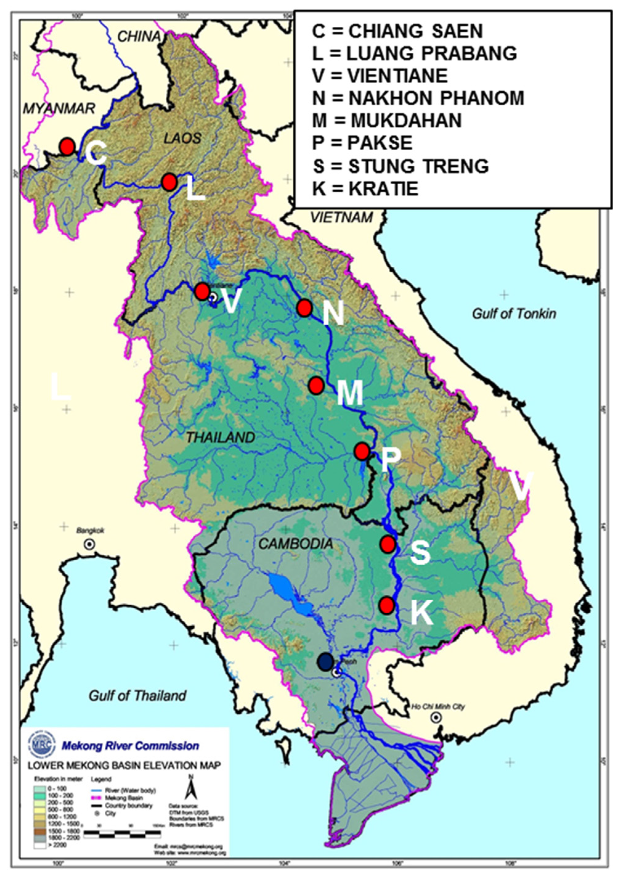
In order to illustrate the concepts of Section 2, data obtained from three models for forecasting Mekong River flows for the middle reach of the Mekong River (see Figure 1) were used. Two data based models, using very different model structures, are taken from Shahzad and Plate, [3]. Here, we add a third model, the persistence model, which is called model 0. Models 1 and 2 were developed by Shahzad [47] using records of daily discharges Qj(i+m) from seven gaging stations j (shown in Figure 1) and rainfall sums for each day i from 37 rainfall stations, which were available for 15 years from 1991 to 2005. Approximate flow times between gages are one or two days. First a basic flow network was set up, which connects all gages j. An algorithm based on the continuity equation was developed [3], which allows the routing of area averaged contributions from the subareas between adjacent stations to reference station 0, where forecasts for up to m = 5 days were made. It is used for both models, which were calibrated using the same observed discharge differences between adjacent upstream gages. The difference between models 1 and 2 lies in their different forecast sub-models for the sub-areas between gages. Model 1 of Shahzad and Plate [3] is a typical time series model. Discharge increments for each sub-area are forecast by regression analysis with known increments of the past. Model 2 is a unit hydrograph rainfall-runoff model for the discharge increments due to runoff from the sub-areas between gages. A special feature of model 2 is the seasonally varying adjustment factor KN, which converts rainfall into effective precipitation. For details, paper [3] should be consulted.
Figure 1.
Middle reach of the Mekong, showing gaging stations (with permission of Mekong River Commission).
Figure 1.
Middle reach of the Mekong, showing gaging stations (with permission of Mekong River Commission).

During calibration empirical parameters of both models were fitted to minimize variances of calibration errors e = Q(i+m) − QF(i+m), assuming Q(i+m) given (from historical data) and QF(i+m) the result of model calculation. In forecast applications, the situation is reversed, forecast QF(i+m) is given, and Q(i+m) is estimated by means of its conditional pdf. The purpose of the present study is to investigate this reverse process and to study effects of various error correction routines. The models originally were applied to all seven stations along the middle Mekong River [3]. In the following, data and model outputs for station Stung Treng, located at the end of the middle reach of the Mekong shown in Figure 1, are used as a reference station, (identified as station j = 0) for illustrating the error analysis of Section 2. For this station, error statistics for all years, from 1991 to 2000, are derived for each forecast time of m days. For illustrations, discharge forecasts for three days ahead for year 1997 at station Stung Treng are used.
3.1. Application of Models 0, Model 1 and Model 0,1
Results from the analysis of errors for all models involving regressions (model 0, model 1 and model 0,1) are summarized in Table 1. Parameters for models listed in Table 1 were calculated from dimensionless discharge data for station Stung Treng for 1991 to 2000. Forecasts QFk(i+m) according to model k were obtained, which yield errors ek. Combinations of models are denoted by index k1,k2. Typical results for forecasts by means of model 1 are shown in Figure 2 for m = 3. Top curves are observed and forecast seasonal discharges, and bottom curves conditional forecast errors: e1 for single model dependency on model 1, e0 shows single model dependency on the persistence model, and e1,0 two model dependency on optimum combination of model 1 and persistence model. Included in Table 1, column 11 is the skew coefficient of the pdf of QF0,1(i+m), and the last column, 12. The skew coefficient is needed for Weibull fitting (see Appendix).

Table 1.
Results from combinations of model 1 and persistence model 0. Column 7 lists standard deviations of calibration error e = Q(i+m) − QF1(i+m), columns 2, 3 and 4 show correlation coefficients for all error equations, column 5 and 6 are parameters for Equation (15). All standard deviations (std) are in m³/s.
| m | a1,0 | b1,0 | std | skew | PIopt | ||||||
|---|---|---|---|---|---|---|---|---|---|---|---|
| e | e0 | e1 | e1,0 | ||||||||
| 1 | 0.991 | 0.996 | 0.996 | 1.157 | −0.162 | 1299 | 1886 | 1299 | 1284 | 0.602 | 0.54 |
| 2 | 0.971 | 0.986 | 0.988 | 1.110 | −0.126 | 2349 | 3350 | 2346 | 2330 | 0.602 | 0.52 |
| 3 | 0.946 | 0.969 | 0.981 | 1.096 | −0.129 | 3450 | 4547 | 3447 | 3429 | 0.568 | 0.43 |
| 4 | 0.919 | 0.949 | 0.973 | 1.045 | −0.099 | 4418 | 5533 | 4415 | 4404 | 0.517 | 0.37 |
| 5 | 0.891 | 0.926 | 0.965 | 0.971 | −0.048 | 5266 | 6355 | 5260 | 5258 | 0.462 | 0.32 |
Figure 2.
Forecast results for m = 3 days with model 0 and model 1 for Stung Treng in 1997.

The resulting forecast hydrograph QF1(i+m) has a shape very similar to that of model 0, as illustrated by means of the two error hydrographs in Figure 2. In both figures, substantial forecast errors are observed, in particular for longer forecast times, and for times with large discharge changes over short times, where model outputs always lag behind observed hydrographs. Outputs of model 1 and of the combination of model 1 and model 0 (model 0,1, not shown) are practically identical, as seen from comparing columns 9 and 10. The reason for this behavior is that both model 1 and model 0 are regression models, and reduce errors in the same way. However, model 1 shaves off some part of the error peaks of the persistence model 0. This, perhaps, is not so evident in Figure 2, but it is documented in the reduction of the standard deviation listed in Table 1, where model averages over all 10 years of records are shown. The standard deviation of error e1 relative to standard deviation of model 0 error e0 is about 68% for m = 2, 76% for m = 3, and 82% for m = 5, leading to persistence indices PI of about 0.3 for m = 5 and of about 0.4 for m = 3.
3.2. Application of Model 2
Two different types of model 2 of Shahzad and Plate [3] are important: model 2.1, which is used to calibrate model 2 with historical input and output data, and model 2.3, which uses the parameters of model 2.1, but with rainfall forecasts (applying the rainfall persistence assumption P(i+r) = P(i), (r = 1,2…m) as rainfall forecast model).
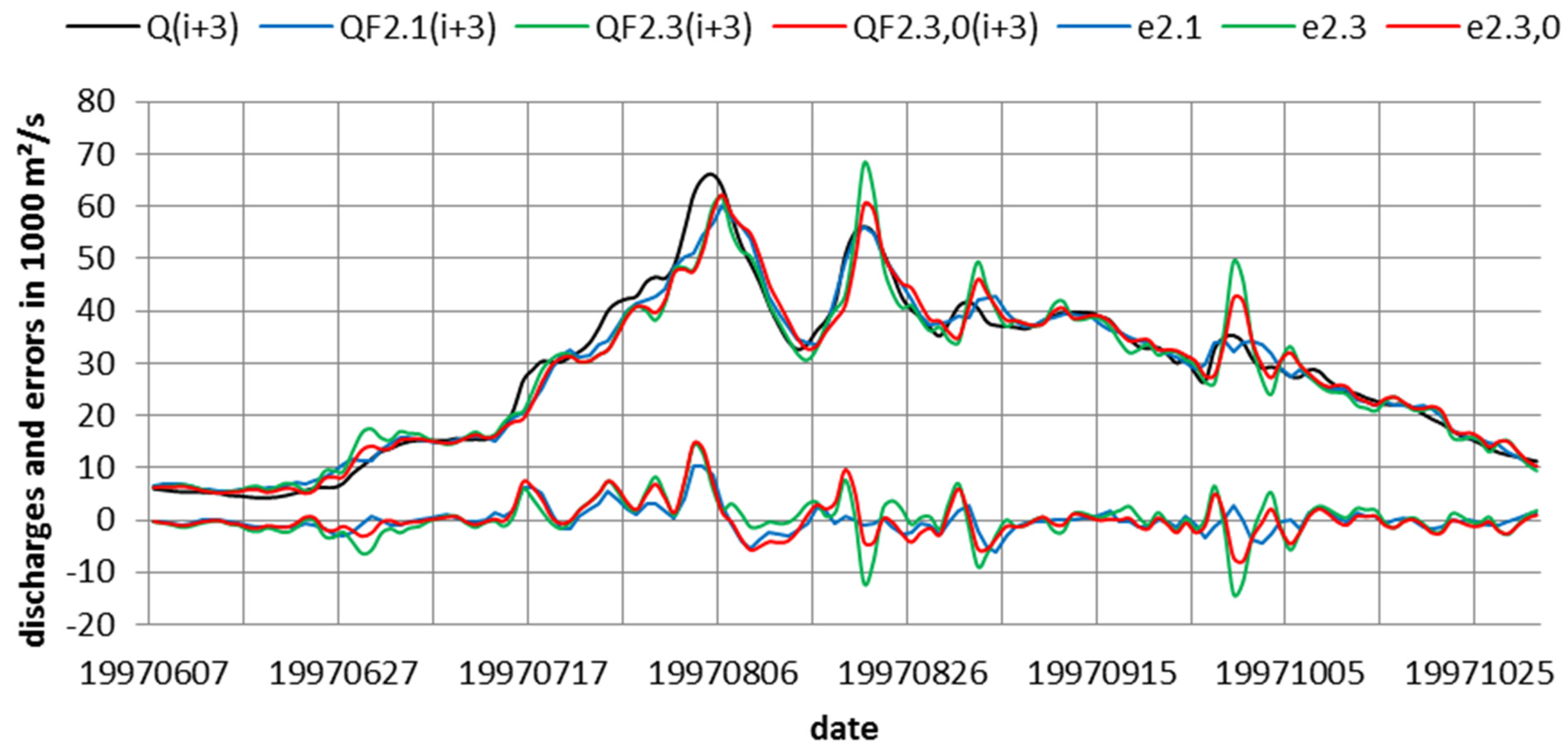
Consider first, application of model 2.3 and the combination of model 0 and model 2.3, yielding forecasts QF2.3,0(i+m). Typical results are shown in Figure 3 for m = 3 for 1997 at gage Stung Treng. By comparing columns 7 and 9 in Table 2 we notice first that standard deviations of calibration errors e are almost the same as conditional forecast errors e2.3, as was also observed in other cases by Todini [48]. In the forecast-hydrograph strong oscillations of QF2.3(i+m) are noted, which are caused by the strong variation of rainfall from day to day. Due to the persistence assumption for rainfall estimation the daily variation of rainfall is fully preserved. The oscillations could be reduced if the rainfall input was smoothed over some time period, i.e., by taking the average of the last three or four days. Such a smoothing filter leads to a reduction of the variance, but also to larger time lags for all stations and all times.
Figure 3.
Forecast results for 3 days with model 2.3 and linear combination of model 2.3 with model 0 for Stung Treng in 1997. Additionally shown is the forecast of model 2.1.
Figure 3.
Forecast results for 3 days with model 2.3 and linear combination of model 2.3 with model 0 for Stung Treng in 1997. Additionally shown is the forecast of model 2.1.

It is evident that inclusion of model 0 in the combined forecasts of model 2.3 and 0 also has such a smoothing effect, as seen in Figure 3. Significantly smaller standard deviations of e0,2.3 as compared with e2.3 are documented in columns 9 and 10 of Table 2. This is reflected in column 12 of Table 2, which shows the improved persistence index for best results, corresponding to curve QF0,2.3(i+3) of Figure 3. As comparison of column 9 and 10 shows, the combination of model 0 with model 2.3, in the multiple regression mode, improves the standard deviation of e0,2.3 by 21 % for m = 1 and 11% for m = 5, yielding improvement of persistence index PI from 0.40 for m = 5 to 0.58 for m = 1 (see column 12).
Table 2.
Results from combinations of model 2.3 and persistence model. Columns 2–4 show parameters (correlation coefficients) for all error equations, column 5 and 6 are parameters for Equation (15). Column 7 lists standard deviations (std) of calibration error e = Q(i+m) − QF1(i+m). All std are given in m³/s.
| m | a2,0 | b2,0 | std | std | std | std | Skew | PIopt | |||
|---|---|---|---|---|---|---|---|---|---|---|---|
| e | e0 | e2.3 | e0, 2.3 | ||||||||
| 1 | 0.996 | 0.991 | 0.994 | 0.910 | 0.087 | 1216 | 1886 | 1215 | 1207 | 0.589 | 0.58 |
| 2 | 0.988 | 0.971 | 0.973 | 0.809 | 0.183 | 2195 | 3350 | 2193 | 2108 | 0.569 | 0.58 |
| 3 | 0.969 | 0.946 | 0.936 | 0.672 | 0.317 | 3478 | 4547 | 3478 | 3105 | 0.563 | 0.53 |
| 4 | 0.939 | 0.918 | 0.891 | 0.587 | 0.395 | 4822 | 5533 | 4809 | 4100 | 0.553 | 0.45 |
| 5 | 0.907 | 0.891 | 0.846 | 0.541 | 0.433 | 5956 | 6355 | 5879 | 4913 | 0.548 | 0.40 |
An advantage of Bayesian analysis for model class 1 type 2 is the separation of model uncertainty of the hydrological model from the uncertainty of the rainfall forecast model, as outlined in Section 2.3.4. Evidently, the difference in discharge forecasts from the two versions of model 2 is attributable to rainfall forecast inaccuracy. The best forecast with model class 2 is obtained with historical rainfall (model 2.1) in combination with forecast from model 1. An analysis of this case shows that the rainfall-runoff model 2.1 with inclusion of model 1 (column 4 of Table 3) is practically the same, with and without model 1 (column 3 of Table 3). Therefore, we use the standard deviations of column 4 as the best model with rainfall known. According to Section 2.3.4, the dimensional variance for model 2.1 is and that for the case with rainfall forecast model 2.3 is with standard deviations of column 6, and of column 3. Fractions of variances attributable to rainfall forecast inaccuracy are summarized in column 7 of Table 3. Errors due to rainfall forecast uncertainty are rapidly increasing with increased forecast time, reaching more than 50% for m = 5, indicating the need for improved rainfall forecasts for larger m, while the model error dominates short times m.
Table 3.
Effect of rainfall forecast on forecast accuracy for combinations of model class 2 type 2.1 and 2.3.
| m | S2·h | Standard Deviations for Different Model Combinations in m³/s | Fraction of Rainfall Uncertainty | ||||
|---|---|---|---|---|---|---|---|
| Persistence Model 0 | Model 2.1 | Combination Model 1 and Model 2.1 | Model 2.3 | Combination Model 1 and Model 2.3 | |||
| 1 | 0.991 | 1886 | 1187 | 1186 | 1215 | 1214 | 0.061 |
| 2 | 0.971 | 3350 | 1942 | 1927 | 2193 | 2051 | 0.155 |
| 3 | 0.946 | 4550 | 2517 | 2498 | 3478 | 2951 | 0.349 |
| 4 | 0.918 | 5533 | 3002 | 2989 | 4809 | 3846 | 0.487 |
| 5 | 0.891 | 6355 | 3398 | 3391 | 5879 | 4638 | 0.574 |
3.3. Application of Model 1 and Model 2 in Combination
The success of combining model 2 type 3 and model 0 suggests using model 1 instead of model 0 as part of a class 2 model, because model 1 and model 0 are both regression models, and model 1 actually is an improved version of model 0. Let this combination be called model 3, with index 1,2.3. Table 3 is a summary of model 3 parameters and standard deviations. It had already been suggested in [3] to use such a combination, and the generalization used here is a logical extension of class 2 error analysis, as it results in weighted averages of both models. The weights are listed in column 5 and 6 of Table 4, with a1,2 the weight given to model 1, and b1,2 the weight for model 2. Weights are seen to shift with increase of m from 0.66 for model 2 type 3 for m = 1 to 0.39 for m = 5.
Table 4.
Results from combinations of model 2 and model l. Columns 2, 3, and 4 show parameters (correlation coefficients) for all error equations, column 5 and 6 are parameters for Equations (7) and (8). All std in m³/s.
| m | a1,2 | b1,2 | std | Skew | PIopt | |||||
|---|---|---|---|---|---|---|---|---|---|---|
| e1 | e2.3 | e1,2.3 | ||||||||
| 1 | 0.996 | 0.996 | 0.998 | 0.334 | 0.662 | 1299 | 1215 | 1214 | 0.596 | 0.59 |
| 2 | 0.988 | 0.986 | 0.989 | 0.579 | 0.413 | 2346 | 2194 | 2051 | 0.584 | 0.63 |
| 2W | 0.987 | 0.989 | 0.991 | 0.398 | 0.595 | - | - | 2023 | 0.572 | |
| 3 | 0.969 | 0.969 | 0.965 | 0.501 | 0.485 | 3447 | 3479 | 2951 | 0.563 | 0.58 |
| 4 | 0.949 | 0.939 | 0.930 | 0.558 | 0.420 | 4415 | 4806 | 3846 | 0.529 | 0.52 |
| 5 | 0.926 | 0.907 | 0.893 | 0.574 | 0.394 | 5260 | 5880 | 4638 | 0.496 | 0.47 |
| 5W | 0.937 | 0.926 | 0.918 | 0.550 | 0.421 | - | - | 4623 | - | 0.47 |
Lines 2W and 5W of Table 4 are results from using linear multiple regression of variables w obtained from transforming originally Weibull distributed data into normal. The method described in Section 2.4.3 is applied to the combination of model 1 and model 2.3. A very small improvement of about 1% in variance reduction was obtained, so small that it does not seem to justify the effort of conversion into normal variables, in particular since no theoretical reason can be given why linear regressions among transformed variables is better than linear regressions among the original variables.
Typical results illustrating model 3 outputs are shown in Figure 4. Bottom curves are conditional forecast errors: e1 for single model dependency on model 1, e2.3 shows single model dependency on model 2.3, and e1,2.3 two model dependency on the optimum combination 1,2.3 of model 1 and model 2.3. The results of column 12, with PI values roughly decreasing from 0.6 for small m to 0.47 for m = 5 are the best results obtainable with the present set of models.
Figure 4.
Forecast results for m = 3 days showing model 1, model 2 type 3, and linear combination of the two models to yield model 1,2.3 for Stung Treng in 1997.
Figure 4.
Forecast results for m = 3 days showing model 1, model 2 type 3, and linear combination of the two models to yield model 1,2.3 for Stung Treng in 1997.

3.4. Probability Densities of Final Errors
Probability densities were found by first normalizing all errors by division through their standard deviation. Their mean was zero in all cases. Then the data were ordered in classes of width 0.5 times standard deviation, relative numbers of values found per class were used as estimators for class probability, and empirical pdfs determined by drawing smooth curves through normalized relative magnitudes.
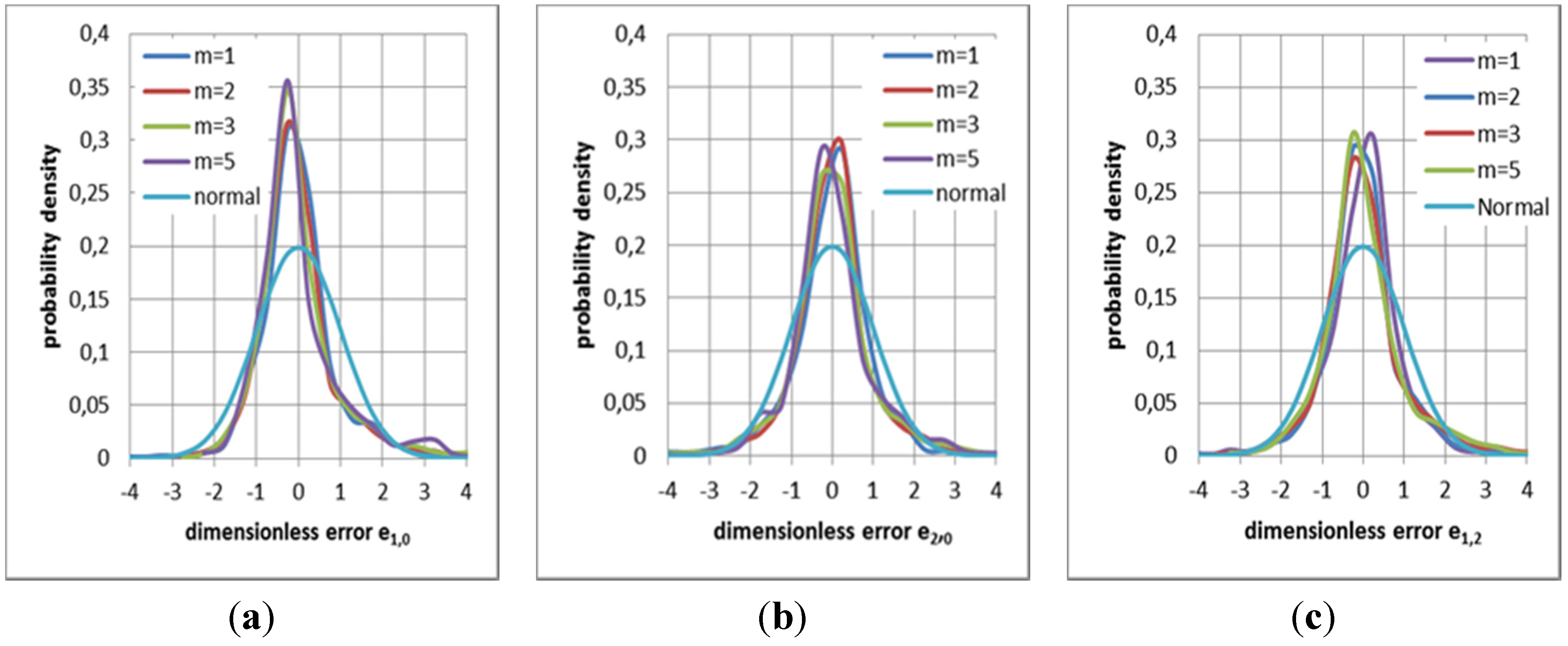
Results for all three optimum types considered in Section 3.1 to Section 3.3 are shown in Figure 5. All data yield shapes distinctly different from normal distributions, also shown in the figures. They are much more concentrated around the center—showing a large proportion of small errors—and are somewhat skewed. Their skew coefficients are listed in columns 11 of Table 1, Table 2, and Table 4. All hydrographs from model 2 show (see Figure 3 and Figure 4) that the largest errors occur due to rapid changes in rainfall input, which is not forecasted by the rainfall model.
Figure 5.
Probability densities of errors for cases of model combinations. (a) pdf of error e1,0; (b) pdf of error e2.3,0; (c) pdf of error e1,2.3.
Figure 5.
Probability densities of errors for cases of model combinations. (a) pdf of error e1,0; (b) pdf of error e2.3,0; (c) pdf of error e1,2.3.

It is a special characteristic of the hydrological regime of the middle Mekong that these changes are difficult to anticipate. Rainfall maxima typically are generated by typhoons moving in from the South China Sea and occur almost simultaneously over large stretches along the Annamite (Truong Son) mountains, which form the boundary between Laos and Vietnam. The catchment characteristic of the middle Mekong are such that, instead of spreading the runoff from these rainfall extrema over time, they are superimposed and lead to large discharge peaks at downstream stations on the middle Mekong. The analysis of the final errors does not consider the heteroscedasticity of the error. Since critical forecasts are associated with strong jumps in the hydrograph, where unfortunately errors are largest, tail ends of distributions are of special significance. It is evident that probabilities for errors larger than two standard deviations are larger than normal. This must be taken into account if weighted decisions based on these tails are to be made.
4. Summary and Conclusions
In this paper, we looked at possible forecast improvements by means of combining two different models. We start with given forecast models, which are supposed to have been developed in a design phase. As an example, we use results from the Mekong River, i.e., the models of Shahzad and Plate [3], as optimum models. Parameters for the models had been optimized by means of historical data as part of design. The parameters are kept constant during forecast.
Due to scarcity of rainfall stations and/or model simplicity, models used for the Mekong River suffer from large inherent uncertainty—the error analysis showed that there is much room for model improvement, in particular if the rainfall forecast could be improved. Under any circumstances one must live with the system error eMk (i+m). It sets the limit of forecast quality. It can be reduced only if model or data base, or both, are improved. For a regression model without forecasted components, such as our model 1, error eMk (i+m) statistics are the same as forecast error eFk(i+m) statistics. For rainfall-runoff models, eMk(i+m) and eFk(i+m) are different: the former obtained with historical forecasts, the latter with forecasts based on rainfall forecast modeling, in our case assuming persistence of rainfall. The variance of eMk(i+m) must be used as reference against which to measure forecast error eFk(i+m), which is obtained in the operational or forecast mode as combination of system error and error due to imperfect forecast of input data. If the difference in the two errors for a given situation is small, then an effort in obtaining better forecast input data offers no big advantage, and the primary effort should be directed to improve the model and/or its parameters. If the difference is large, a major effort is needed for improving the forecast of the input data. The large differences of the outputs of models 2.1 (yielding eMk(i+m)) and model 2.3 (yielding eFk(i+m)) indicate that much could be gained for forecasts with the simple unit hydrograph model 2 if better rainfall forecasts were available.
The error analysis proceeds along concepts developed by Krzysztofowicz. Operational forecasts are identified as depending on the set of conditions existing at the time of forecasting, such as discharge or rainfall data at time i. This concept permits to combine contributions of different models in a logical and systematic fashion. We used three models: the simple persistence model 0 (assuming QF(i+m) =Q(i)), model 1, which is a regression model based on regressing discharge QF(i+m) on inputs from upstream reaches, and model 2, which is a rainfall-runoff model. Results of the error analysis showed that the best results were obtained by means of model 2.3 combined with model 1. The original data are well fitted by Weibull distributions, but no advantage was found from converting these data into normally distributed data, which after conversion are linearly correlated, as had been suggested by Krzysztorowicz [1].
An interesting observation is that the contribution of h0 to the forecast pdf is much smaller for model 1 than for model 2, although from a direct comparison it would seem that the larger uncertainty of model 1 would make it more likely that a contribution of h0 would matter. The reason for this behavior is that model 1 is a regression model, and the forecast for model 1 is more likely than model 2 to be comparable to the forecast from the persistence model, which also is a (rather elementary) regression model. Therefore one may conclude that the regression property of model 0 is already included in the general regression model, so that h0 can make only a small contribution to the forecast by means of model 1. On the other hand, model 2 does not have a regression component. Therefore, model 0 complements the forecast from the rainfall-runoff model. This may imply that the use of a rainfall-runoff model profits more from the inclusion of h0-dependency than a regression model.
Acknowledgments
Figure 1 and the basic data for the analysis were made available for scientific purposes by the Mekong River Commission (MRC). Cooperation with the Operations Unit of the MRC’s Regional Flood Management and Mitigation Center is gratefully acknowledged. Thanks for financial support go to DAAD (German Academic Exchange Service), Higher Education Commission of Pakistan, and the German Ministry of Science and Technology under project WISDOM. The senior author gratefully acknowledges the initiation of this research through a correspondence with E. Todini.
Author Contributions
The analysis was done and paper was written by Erich J. Plate, data and basic calculations were supplied by Khurram M. Shahzad.
Conflicts of Interest
The authors declare no conflict of interest.
Appendix
A Method of Fitting Weibull Distributions to Data
Krzysztofowicz and his students [1,43,45] recommend use of 3-parameter Weibull distribution functions Fx with pdf fx for variables h, h0 and s1, which may be written (for any variable x):
For determination of parameters α, 𝛽 and x0 three statistical parameters, mean, variance and skew coefficient are needed. Mean and variance of variables h, s1, and h0 are 0 and 1, respectively, and skew coefficients (where M3 is the third central moment and M2 the variance of variable x) can be calculated from data. Relationships between statistical moments and parameters of the Weibull distribution consist of functions of Gamma functions and cannot be solved explicitly. A semi-graphic method was developed in Plate [44] which is based on the fact that parameter α of Equation (A-1) depends on Csx only. Pairs of corresponding values of α and Csx are tabulated, and a universal diagram showing and as functions of 1/α is given in [44]. With α known, the two parameters 𝛽 and are determined from the universal diagram. With these parameter is calculated, and by setting normal variables with mean and variance of the untransformed variable x are obtained.
References
- Krzysztofowicz, R. Bayesian system for probabilistic river stage forecasting. J. Hydrol. 2002, 268, 16–40. [Google Scholar] [CrossRef]
- Todini, E. From HUP to MCP: Analogies and extended performances. J. Hydrol. 2013, 477, 33–42. [Google Scholar] [CrossRef]
- Shahzad, M.K.; Plate, E.J. Flood forecasting for River Mekong with data-based models. Water Resour. Res. 2014, 50, 7115–7133. [Google Scholar] [CrossRef]
- Todini, E. A model conditional processor to assess predictive uncertainty in flood forecasting. Int. J. River Basin Manag. 2008, 6, 123–137. [Google Scholar] [CrossRef]
- Singh, V.J.; Woolhiser, D.A. Mathematical modeling of watershed hydrology. J. Hydrol. Eng. ASCE 2000, 7, 270–291. [Google Scholar] [CrossRef]
- Gouweleeuw, B.; Reggiani, P.; de Roo, A. A European Flood Forecasting System EFFS; European Report EUR 21 208; Office for Official Publications of the European Communities: Luxembourg, 2004. [Google Scholar]
- Wu, C.L.; Chau, K.W. Rainfall-runoff modeling using artificial neural network coupled with singular spectrum analysis. J. Hydrol. 2011, 309, 394–409. [Google Scholar] [CrossRef]
- Kachroo, R.K.; Liang, G.C. River flow forecasting. Part 2: Algebraic development of linear modeling techniques. J. Hydrol. 1992, 133, 17–40. [Google Scholar]
- Blöschl, G. Hydrological synthesis: Across processes, places, and scales. Water Resour. Res. 2006, 42. [Google Scholar] [CrossRef]
- Plate, E.J. Classification of hydrological models for flood management. J. Hydrol. Earth Syst Sci. HESS 2009, 13, 1–13. [Google Scholar]
- Fenicia, F.; Savenije, H.H.G.; Matgen, P.; Pfister, L. Understanding catchment behavior through stepwise model concept improvement. Water Resour. Res. 2008, 44. [Google Scholar] [CrossRef]
- Clarke, R.T. Uncertainty in the estimation of mean annual flood due to rating-curve indefinition. J. Hydrol. 1999, 222, 185–190. [Google Scholar] [CrossRef]
- Krzysztofowicz, R. Why should a forecaster and a decision maker use Bayes theorem? Water Resour. Res. 1983, 19, 327–336. [Google Scholar] [CrossRef]
- Martina, M.L.V.; Todini, E.; Libraton, A. A Bayesian decision approach to rainfall thresholds based flood warning. J. Hydrol. Earth Syst Sci. HESS 2006, 10, 413–426. [Google Scholar] [CrossRef]
- Singh, S.K.; Liang, J.; Bárdossy, A. Improving the calibration strategy of the physically-based model WaSiM-ETH using critical events. Hydrol. Sci. J. 2012, 57, 1487–1505. [Google Scholar] [CrossRef]
- Beven, K.J.; Freer, J.E. Equifinality, data assimilation, and uncertainty estimation in mechanistic modeling of of complex environmental systems using the GLUE method. J. Hydrol. 2001, 249, 11–29. [Google Scholar] [CrossRef]
- Beven, K.J.; Binley, A. The future of distributed models: Model calibration and uncertainty prediction. Hydrol. Process. 1992, 6, 279–288. [Google Scholar] [CrossRef]
- Freer, J.; Beven, K.J.; Ambroise, B. Bayesian estimation of uncertainty in runoff prediction and the value of data. An application of the GLUE approach. Water Resour. Res. 1996, 32, 2161–2173. [Google Scholar] [CrossRef]
- Gupta, H.V.; Sorooshian, S.; Yapo, P.O. Toward improved calibration of hydrological models: Multiple and non-commensurable measures of information. Water Resour. Res. 1998, 34, 751–763. [Google Scholar] [CrossRef]
- Hundecha, Y.; Ouarda, T.; Bárdossy, A. Regional estimation of parameters of a rainfall-runoff model at ungauged watersheds using the spatial structures of the parameters within a canonical physiographic-climatic space. Water Resour. Res. 2007. [Google Scholar] [CrossRef]
- Thiemann, M.; Trosset, M.; Gupta, H.; Sorooshian, S. Bayesian recursive parameter estimation for hydrological models. Water Resour. Res. 2001, 37, 2521–2535. [Google Scholar] [CrossRef]
- Marshall, L.; Sharma, A.; Nott, D. Modeling the catchment via mixtures: Issues of model specification and validation. Water Resour. Res. 2006, 42. [Google Scholar] [CrossRef]
- Krishnamurti, T.N.; Kishtawal, C.M.; LaRow, T.E.; Bachiochi, D.R.; Zhang, Z.; Williford, C.E.; Gadgil, S.; Surendran, S. Improved weather and seasonal climate forecasts from multimodel superensemble. Science 1999, 285, 1548–1550. [Google Scholar] [CrossRef] [PubMed]
- Werner, M.G.F.; van Dijk, M.; Schellekens, J. DELFT-FEWS: An open shell flood forecasting system. In Proceedings of the 6-th International Conference on Hydroinformatics, Singapore, 21–24 June 2004; World Scientific Publishing Co.: Singapore, 2004; pp. 1205–1212. [Google Scholar]
- Brath, A.; Montanari, A.; Toth, E. Neural networks and non-parametric methods for improving real-time flood forecasting through conceptual hydrological models. J. Hydrol. Earth Syst Sci. HESS 2002, 6, 627–640. [Google Scholar] [CrossRef]
- Burlando, P.; Rosso, R.; Cadavid, L.G.; Salas, J.D. Forecasting of short-term rainfall using ARMA models. J. Hydrol. 1993, 144, 193–211. [Google Scholar] [CrossRef]
- Toth, E.; Brath, A. Multistep ahead streamflow forecasting: Role of calibration data in conceptual and neural network modeling. Water Resour. Res. 2007, 43. [Google Scholar] [CrossRef]
- Hsu, K.-L.; Gupta, H.V.; Gao, X.G.; Sorooshian, S.; Imam, B. Self-organizing linear output map (SOLO), an artificial neural network suitable for hydrologic modeling and analysis. Water Resour. Res. 2002, 38, 1302–1314. [Google Scholar] [CrossRef]
- Dawson, C.W.; Abraham, R.J.; Shamseldin, A.Y.; Wilby, R.L. Flood estimation at ungauged sites using artificial neural networks. J. Hydrol. 2006, 319, 391–409. [Google Scholar] [CrossRef]
- Moradkhani, H.; Hsu, K.; Gupta, H.V.; Sorooshian, S. Improved Streamflow Forecasting Using Self-Organizing Radial Basis Function Artificial Neural Networks. J. Hydrol. 2004, 295, 246–262. [Google Scholar] [CrossRef]
- Damrath, U.; Doms, G.; Frühwald, D.; Heise, E.; Richter, B.; Steppeler, J. Operational quantitative precipitation forecasting at the German Weather Service. J. Hydrol. 2000, 239, 260–285. [Google Scholar] [CrossRef]
- Majewski, D.; Liermann, D.; Prohl, P.; Ritter, B.; Buchhold, M.; Hanisch, T.; Paul, G.; Wergen, W.; Baumgardner, J. The operational global icosahedral-hexagonal grid point model GME: Description and high resolution tests. Mon. Wea. Rev. 2002, 130, 319–338. [Google Scholar] [CrossRef]
- Jaun, S.; Ahrens, B. Evaluation of a probabilistic hydrometeorological forecasting system. Hydrol. Earth Syst. Sci. 2009, 13, 1031–1043. [Google Scholar] [CrossRef]
- Marsigli, C.; Boccanera, F.; Montani, A.; Paccagnella, T. The COSMO-LEPS mesoscale ensemble system: Validation of the methodology and verification. Nonlinear Process. Geophys. 2005, 12, 527–536. [Google Scholar] [CrossRef]
- Legates, D.R.; McCabe, G.J., Jr. Evaluating the use of goodness of fit measures in hydrology and hydroclimatic model validation. Water Resour. Res. 1999, 33, 233–241. [Google Scholar] [CrossRef]
- Pappenberger, F.; Ramos, M.H.; Cloke, H.L.; Wetterhall, F.; Alfieri, L.; Bogner, K.; Mieller, A.; Salamon, P. How do I know if my forecasts are better? Using benchmarks in hydrological ensemble prediction. J. Hydrol. 2015, 522, 697–713. [Google Scholar] [CrossRef]
- Bogner, K.; Pappenberger, F. Multiscale error analysis, correction, and predictive uncertainty estimation in flood forecasting systems. Water Resour. Res. 2011, 47, 1–24. [Google Scholar] [CrossRef]
- Gupta, H.V.; Kling, H.; Yilmaz, K.K.; Martinez, G.F. Decomposition of the mean squared error and NSE performance index criteria: Implications for hydrological modeling. J. Hydrol. 2011, 377, 80–91. [Google Scholar] [CrossRef]
- Kitanides, P.; Bras, R. Real time area forecasting with a conceptual hydrological model. 1. Analysis of uncertainty. Water Resour. Res. 1980, 16, 1025–1033. [Google Scholar] [CrossRef]
- Wilks, D.S. Statistical Methods in the Atmospheric Sciences, 2nd ed.; Academic Press: Amsterdam, The Netherlands, 2006; p. 627. [Google Scholar]
- Bürger, G.; Reusser, D.; Kneis, D. Early flood warnings from empirical (expanded) downscaling of the full ECMWF Ensemble Prediction System. Water Resour. Res. 2009, 45. [Google Scholar] [CrossRef]
- Dowell, C.A. Weather forecasting by humans—Heuristics and decision making. Weather Forecast. 2004, 19, 1115–1126. [Google Scholar] [CrossRef]
- Krzysztofowicz, R. Bayesian theory of probabilistic forecasting via deterministic hydrological models. Water Resour. Res. 1999, 35, 2739–2750. [Google Scholar] [CrossRef]
- Plate, E.J. Statistik und Angewandte Wahrscheinlichkeitslehre für Bauingenieure; Ernst & Sohn: Berlin, Germany, 1993; p. 685. (in German) [Google Scholar]
- Krzysztofowicz, R.; Herr, H.D. Hydrologic uncertainty processor for probabilistic river stage forecasting: Precipitation dependent model. J. Hydrol. 2001, 249, 46–68. [Google Scholar] [CrossRef]
- Gelman, A.; Carlin, J.B.; Stern, H.S.; Rubin, D.B. Bayesian Data Analysis; Taylor & Francis Group: Boca Raton, FL, USA, 2003. [Google Scholar]
- Shahzad, K.M.; Karlsruhe Institute of Technology, Karlsruhe, Germany. A data based flood forecasting model for the Mekong River. Unpublished Dissertation. 2011. [Google Scholar]
- Todini, E. Hydrological catchment modelling: Past, present and future. J. Hydrol. Earth Syst. Sci. HESS 2007, 11, 468–482. [Google Scholar] [CrossRef]
© 2015 by the authors; licensee MDPI, Basel, Switzerland. This article is an open access article distributed under the terms and conditions of the Creative Commons by Attribution (CC-BY) license (http://creativecommons.org/licenses/by/4.0/).
Share and Cite
MDPI and ACS Style
Plate, E.J.; Shahzad, K.M. Uncertainty Analysis of Multi-Model Flood Forecasts. Water 2015, 7, 6788-6809. https://doi.org/10.3390/w7126654
AMA Style
Plate EJ, Shahzad KM. Uncertainty Analysis of Multi-Model Flood Forecasts. Water. 2015; 7(12):6788-6809. https://doi.org/10.3390/w7126654
Chicago/Turabian StylePlate, Erich J., and Khurram M. Shahzad. 2015. "Uncertainty Analysis of Multi-Model Flood Forecasts" Water 7, no. 12: 6788-6809. https://doi.org/10.3390/w7126654