Assessment of Suspended Sand Availability under Different Flow Conditions of the Lowermost Mississippi River at Tarbert Landing during 1973–2013

Abstract

Rapid land loss in the Mississippi River Delta Plain has led to intensive efforts by state and federal agencies for finding solutions in coastal land restoration in the past decade. One of the proposed solutions includes diversion of the Mississippi River water into drowning wetland areas. Although a few recent studies have investigated flow-sediment relationships in the Lowermost Mississippi River (LmMR, defined as the 500 km reach from the Old River Control Structure to the river’s Gulf outlet), it is unclear how individual sediment fractions behave under varying flow conditions of the river. The information can be especially pertinent because the quantity of coarse sands plays a critical role for the Mississippi-Atchafalaya River deltaic development. In this study, we utilized long-term (1973–2013) records on discharge and sediments at Tarbert Landing of the LmMR to assess sand behavior and availability under different river flow regimes, and extreme sand transport events and their recurrence. We found an average annual sand load (SL) of 27.2 megatonnes (MT) during 1973 and 2013, varying largely from 3.37 to 52.30 MT. For the entire 41-year study period, a total of approximately 1115 MT sand were discharged at Tarbert Landing, half of which occurred during the peak 20% flow events. A combination of intermediate, high and peak flow stages (i.e., river discharge was ≥18,000 cubic meter per second) produced about 71% of the total annual SL within approximately 120 days of a year. Based on the long-term sediment assessment, we predict that the LmMR has a high likelihood to transport 4 to 446 thousand tonnes of sand every day over the next 40 years, during which annual sand loads could reach a maximum of 51.68 MT. Currently, no effective plan is in place to utilize this considerably high sand quantity and we suggest that river engineering and sediment management in the LmMR consider practices of hydrograph-based approach for maximally capturing riverine sediments.

1. Introduction

River deltas comprise approximately five percent of the Earth’s total land area and over 500 million people reside in them [1,2]. They are important regions in both economic and environmental perspectives as they act as commercial centers and also provide a plethora of natural resources [3,4]. However, many river deltas around the world are facing land loss as the consequence of human and natural factors including river engineering [5,6], accelerated subsidence [7,8], reduced riverine sediment supply [6,9,10], disconnection of the river with its floodplains [11], coastal land erosion [12], and relative sea level rise [13].

One renowned example of river deltas facing land loss problems is the Mississippi River Delta Plain (MRDP) in the southern USA. The MRDP has been losing a substantial amount of land since the early 20th century [6,7,14,15]. A recent study on MRDP land loss [16] reported a disappearing rate of 43 km²/year since 1985. Potential of the MRDP land loss due to river engineering has long been recognized. More than a century ago, Corthell [17] already warned: “If certain levee structures were placed in a manner that fresh water and sediments, along with vital nutrients, were laid to waste off the mouth of the Mississippi River, their deltaic regenerative properties would be lost and unrecoverable.” However, the land loss issue captured major public attention only from the late 1970s (e.g., [7,14,15,18]). During the last decade, in the wake of Hurricane Katrina, there has been an increasing concern over the issue in general public and scientific communities, which led to intensive efforts by the state and federal governments for finding solutions in offsetting coastal land loss [19,20]. One such solution is diversion of the Mississippi River for outsourcing the river water and sediments to coastal marshes for stabilizing the deltaic system. The United States Army Corps of Engineers (USACE) has constructed three notable river diversions in the lowermost Mississippi River reach, namely, Caernarvon (river kilometer, or rk 131), Davis Pond (rk 190) and West Bay (rk 8), of which only West Bay focuses solely on sediment retention and capture [21]. In addition, the State of Louisiana’s Master Plan for coastal restoration (2012) proposed six large to small water (discharge from 141 to 7079 cubic meter per second, or cms) and sediment diversions [20,22], which are still in different planning phases.

Recent reports suggested that the three executed diversions have not gained significant steps towards their objectives despite careful planning and several years of operation [23,24]. The Caenarvon and Davis Pond freshwater diversions have not induced significant salinity reduction [24,25] and have been subjected to more vegetation loss and nutrient overloading post hurricanes Katrina and Rita [24,26]. Similarly, the planned discharge of the West Bay diversion has been increased from 396 cms at its inception in 2003 to 765 cms currently at the cost of adverse effects in navigational route; however, it has not produced desired land growth in the surrounding area [23,27,28].

A primary goal of the river diversion focusing entirely on sediment retention and capture is to divert flow carrying the maximum amount of sediments into adjoining drowned areas for delta restoration without hampering the ecological, structural, hydrological and functional integrity of the river at all [20,22,29]. In the context of this goal, Rosen and Xu [21] analyzed the flow-sediment relationship for Tarbert Landing of the Lowermost Mississippi River (abbreviated hereafter as LmMR and defined as the 500-km reach from the Old River Control Structure to the river’s Gulf outlet) to quantify sediment loads carried by varying flows during 1980–2010. They found that about half of the total annual sediment yield was produced within about 120 days every year when the river was at intermediate (18,000–25,000 cms) and high (25,000–32,000 cms) flows; hence, they recommended these flows to be diverted according to their natural cycle of occurrence during the year. Allison et al. [30] quantified short-term sediment budgets for different locations along the LmMR and suggested that years with high annual flow yielded high sediment input in the system and vice-versa, highlighting the advantage of sediment diversions during high flows.

Suspended solids in the Mississippi River have been found to be composed of a high proportion of fine clay/silt particles (<0.0625 mm) and a low proportion of coarser particles (>0.0625 mm) [30,31]. Studies by Nepf [32] and Nittrouer et al. [33] postulated that sand may play a much more critical role in new land building in the Mississippi River delta than fine clay/silt. The importance of sand transport for the Mississippi River deltaic development has been increasingly recognized [33,34,35,36]. Therefore, analysis of the relationship of total suspended sediment with river hydrology alone is not enough for developing effective sediment management plans. Although the sediment assessments by Rosen and Xu [21], Allison et al. [30] and Nittrouer and Viparelli [36] provide critical information for understanding sediment availability in the LmMR, they give little insights into the actual quantity of riverine sand under different flow regimes. The information about the actual sand availability can be crucial for developing management practices in maximizing sand capture in the LmMR. Understanding the sand–discharge relationship for the LmMR not only is urgent for the river itself but also can help in providing reference information for riverine sediment analysis and coastal land restoration in other sinking river deltas in the world. Furthermore, understanding riverine sand behavior under different flow regimes is also important for research on future river engineering and coastal restoration in combating land loss due to climate-change induced sea level rise.

This study aims to determine sand availability under different flow regimes at Tarbert Landing of the LmMR from 1973 to 2013. The site provides the longest, most regular and most updated discharge and sediment records in the LmMR. Hence, comprehensive study of flow-sediment interaction at this site is important for effective execution and planning of implemented and proposed diversion projects. The specific objectives of the study include: (1) assessing hydrologic effects on sand transport; (2) quantifying daily sand loads and analyzing their seasonal and annual trends; (3) developing a hydrograph-based sand availability scheme for five river stages classified by the U.S. National Oceanic and Atmospheric Administration (NOAA); and (4) assessing extreme events of sand transport and their recurrence. NOAA uses stage records from the Red River Landing site, approximately 1.5 km downstream of the Tarbert Landing gauge station, for its flood warning prediction of the LmMR, whereby five flow stages are classified [37]: (1) Low Flow Stage (river stage: <9.8 m); (2) Action Flow Stage (river stage: 9.8–12.1 m); (3) Intermediate Flow Stage (river stage: 12.1 to 14.6 m); (4) High Flow Stage (river stage: 14.6 to 16.8 m); and (5) Peak Flow Stage (river stage: >16.8 m).

This study mainly focuses on analysis of sand concentration trends across low, medium and high discharge regimes, development of discharge-sand rating curves to calculate sand load for each day at Tarbert Landing from 1973 to 2013 and identification of discharge regimes transporting highest amount of sands. Apart from this, daily discharge has also been analyzed by identifying its monthly and annual trends and its duration curve. Daily discharge analysis is crucial for identifying its short-and long-term relationship with sand transport in the LmMR.

2. Methods

2.1. Study Site

The Tarbert Landing river gauge station (31°00’30” N, 91°7’25” W) is located at river kilometer 493 (river mile 306.3) of the Mississippi River. The station is below the Old River Control Structure (ORCS) [38] (Figure 1) that diverts approximately 25% (under the normal flow conditions) of the Mississippi River’s water into the Atchafalaya River. The site provides the most updated and most comprehensive sediment records for the LmMR where both the United States Geological Survey (USGS) and United States Army Corps of Engineers (USACE) have a monitoring station (USGS Station ID: 07295100 and USACE Gauge ID: 01100). ORCS was built in 1963 with the primary goal of preventing a large amount of Mississippi River water (>30%) from entering the Atchafalaya River [39,40]. Discharge at Tarbert Landing is, therefore, manipulated by ORCS based on specific river flow conditions.

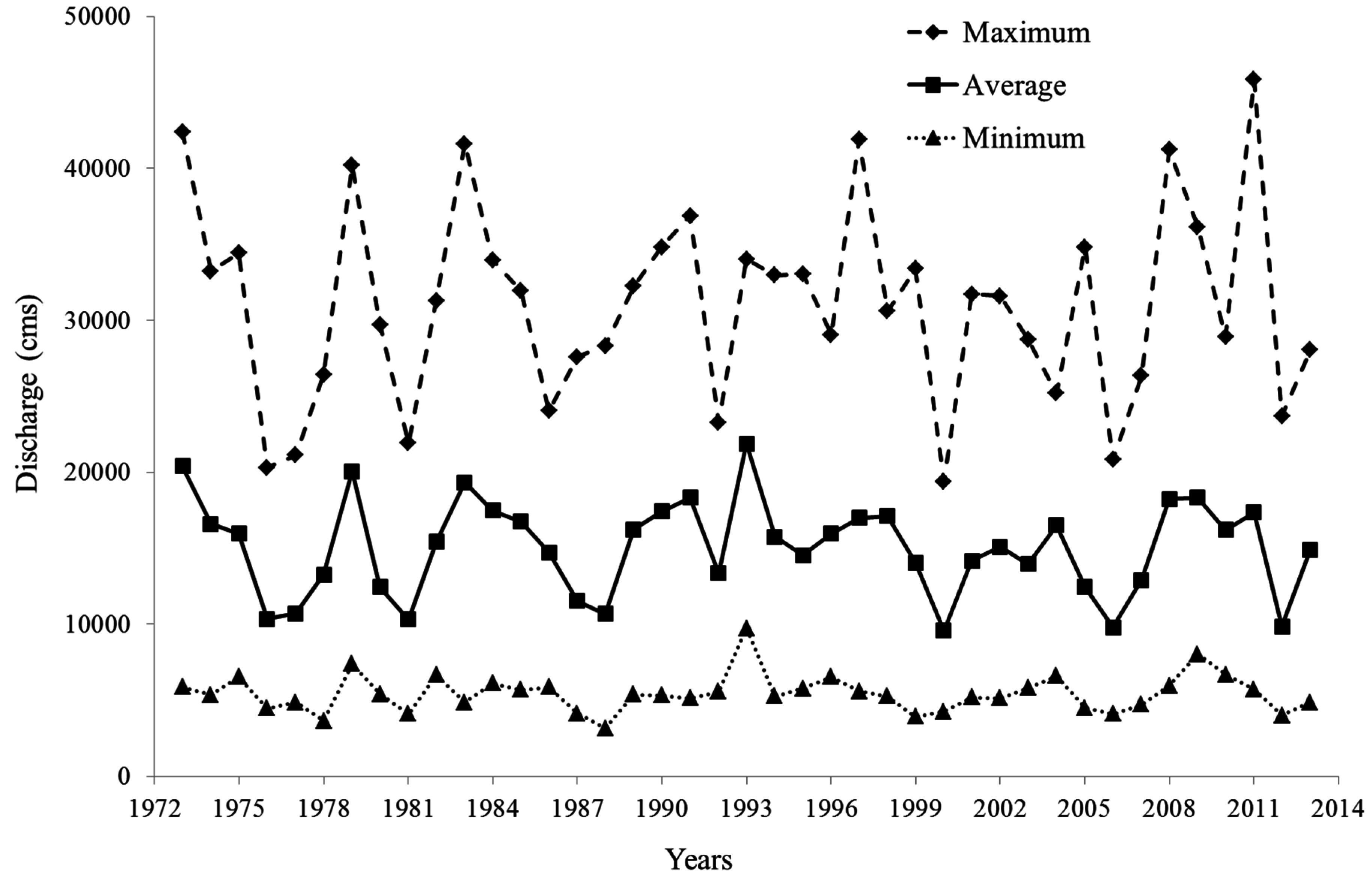
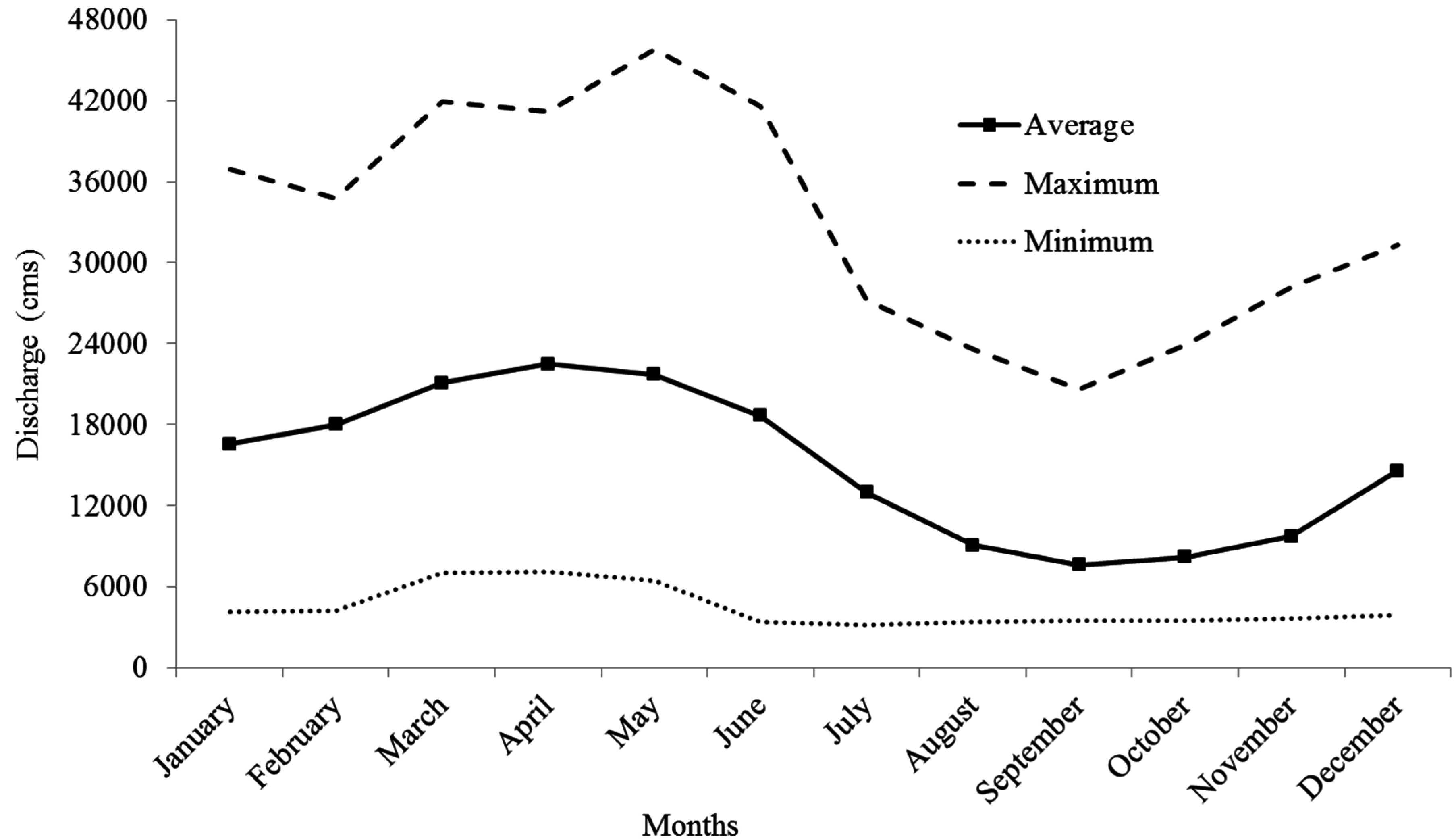
2.2. Flow and Sediment Concentration Data

Records on mean daily discharge (Q_d in cms) were collected for Tarbert Landing from USACE for the period from 1 January 1973 to 31 December 2013. For the same period, measurements on suspended sediment concentrations (SSC) in milligram per liter (mg/L) and corresponding percentage of silt/clay (fine sediment) fractions in SSC (i.e., diameter < 0.0625 mm) were collected from USGS. USGS carries out depth-integrated suspended sediment sampling every 12 to 26 days using several isokinetic point samplers (i.e., P-61, P-63, D-96, D-99) ranging from four to eight verticals and each vertical consisting of two to five samples ([10,41,42,43]—these studies also cover in depth analysis of SSC collection and processing techniques and error adjustments). From 1973 to 2013, a total of 1043 SSC samples were collected, processed and documented for Tarbert Landing. During these 41 years, each month had 1 to 3 sampling dates; therefore, it is assumed that the SSC data have a sufficient, unbiased representation across all seasons and flow regimes. The discharge and sediment concentration data were used to compute sand loads as described in section 2.5 below.

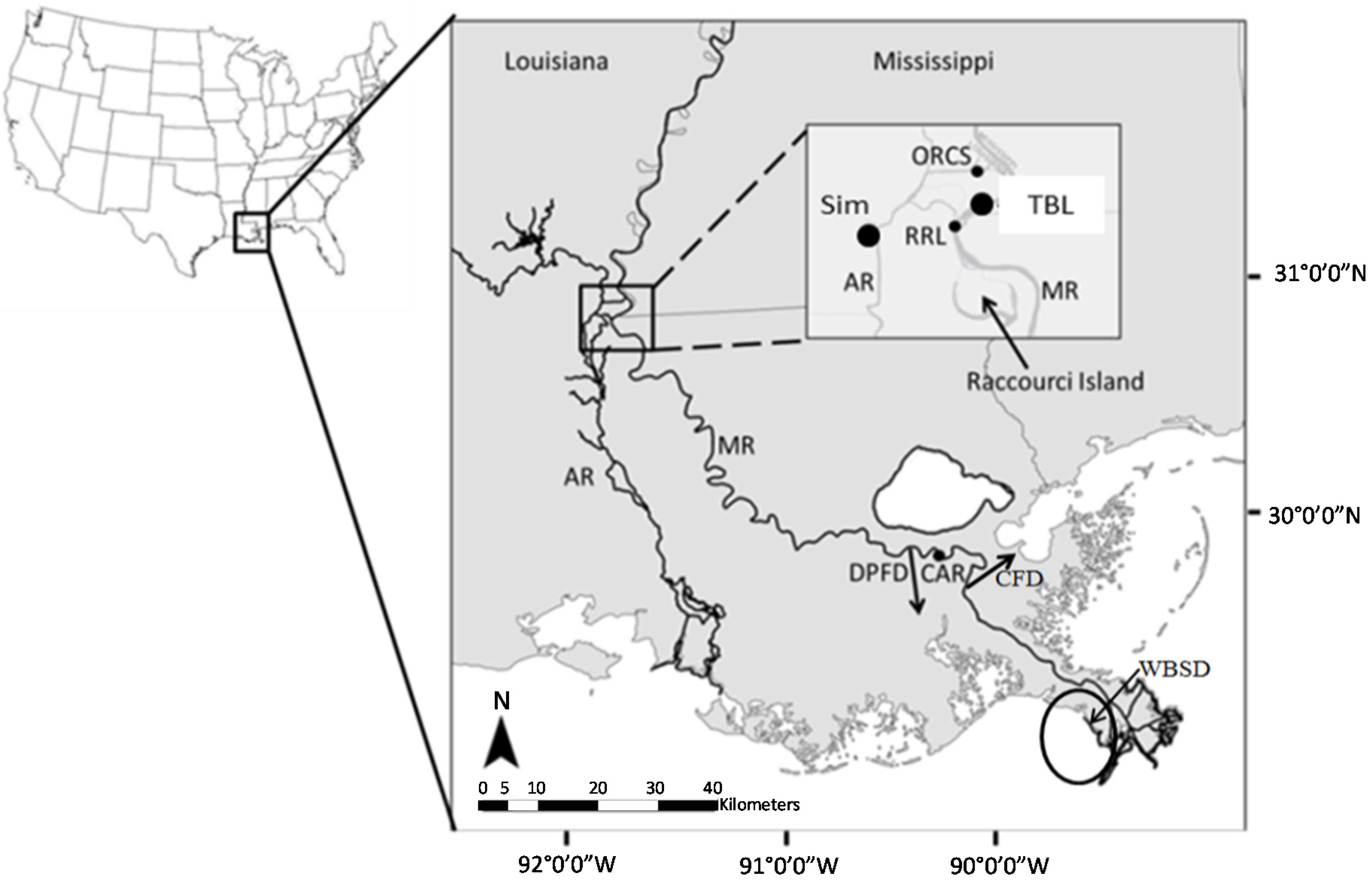
Figure 1. Study area map (modified from Rosen and Xu [21]) showing the location of the LmMR at Tarbert Landing (TBL) (USGS Station ID 07295100 and USACE Gage ID 01100). MR and AR denote the courses of the Mississippi and Atchafalaya Rivers respectively; ORCS is the Old River Control Structure; “Sim” denotes Simmesport (USGS Station ID 07381490) site of the Atchafalaya River; RRL is Red River Landing, the gauging station for USGS just below TBL consisting of river stage records and CAR denotes Carrolton, New Orleans. The three Mississippi River diversions introduced earlier have also been shown in the figure: Davis Pond Freshwater Diversion (DPFD), Caernarvon Freshwater Diversion (CFD) and West Bay Sediment Diversion (WBSD).

Figure 1. Study area map (modified from Rosen and Xu [21]) showing the location of the LmMR at Tarbert Landing (TBL) (USGS Station ID 07295100 and USACE Gage ID 01100). MR and AR denote the courses of the Mississippi and Atchafalaya Rivers respectively; ORCS is the Old River Control Structure; “Sim” denotes Simmesport (USGS Station ID 07381490) site of the Atchafalaya River; RRL is Red River Landing, the gauging station for USGS just below TBL consisting of river stage records and CAR denotes Carrolton, New Orleans. The three Mississippi River diversions introduced earlier have also been shown in the figure: Davis Pond Freshwater Diversion (DPFD), Caernarvon Freshwater Diversion (CFD) and West Bay Sediment Diversion (WBSD).

2.3. NOAA’s River Stages and their Corresponding Flow Regimes

For its flood warning prediction, NOAA defined five river stages at Red River Landing. In their study on long-term suspended sediment transport at Tarbert Landing, Rosen and Xu [21] identified corresponding discharge for these stages: discharge <13,000 cms for Low Flow Stage, 13,000–18,000 cms for Action Flow Stage, 18,000–25,000 cms for Intermediate Flow Stage, 25,000–32,000 cms for High Flow stage, and >32,000 cms for Peak Flow Stage. These regimes were further used several times in our study, e.g., in frequency analysis, duration curves, and sand distribution and transport trends across these regimes.

2.4. Sand Concentration in River Discharge

Using the percentage of silt/clay fractions in suspended sediment concentration, we first calculated silt/clay concentration (SSC_f) by multiplying the percentage with SSC. Sand concentration (SSC_s in mg/L) for each sampling event was then quantified by subtracting the SSC_f (mg/L) from SSC (mg/L). The distribution of SSC_s across a daily river discharge (Q_d) range was then analyzed by building two types of SSC_s (y-axis)-Q_d (x-axis) plots: P-1 and P-2. Average SSC_s and their percentage changes within pre-selected Q_d intervals (every 3000 cms) were plotted against those Q_d intervals in P-1. Similarly, individual SSC_s were fitted against their corresponding Q_ds in P-2. The upper limit of the Q_d range in P-1 after which average SSC_s began to decrease following a continuous increase (27,000 cms) gave the point for separating increasing and decreasing SSC_s in P-2. Hence, all SSC_s values for Q_d ≤ 27,000 cms were defined as increasing sand, while all SSC_s values for Q_d > 27,000 cms were defined as decreasing sand in P-2.

2.5. Development of Discharge-Sand Load Rating Curves

Daily sand load (DSL in tonnes/day) was computed by multiplying SSC_s with the corresponding daily discharge (Q_d in cms) for all the sampling dates during 1 January 1973 and 31 December 2013 as:

$$DSL=Q_d\times SS{C}_s\times 0.0864$$

(1)

where 0.0864 is a unit conversion factor for converting the sand mass to tonnes per day.

There were nine outliers out of a total of 1043 sediment sampling events for the entire 41-year study period. These ~1% outliers were four to six times higher than the long-term standard deviation of sand concentrations; hence, we decided to remove them from further analysis. Now, a natural logarithm (ln) was taken for the two variables, DSL (dependent; y) and Q_d (independent; x), and both linear and polynomial rating curves were applied for the relation between them. The evaluation of all applied rating curves were based on four criteria: regression coefficient of the curves (R² must be ≥0.8), root mean square errors of the predicted (or calculated) DSLs (RMSE) (the lower the better), standard error (SE) of the rating curves (in ln units) (also, the lower the better) and a graphical assessment (good visual agreement between corresponding calibrated and predicted DSLs) [44,45,46].

To achieve the “predicted DSLs”, we fitted “log transformed (ln) Q_ds” in the rating curve equations to get “predicted ln DSLs” at first and then transformed back thus obtained “predicted ln DSLs” by taking their exponential values. We also checked potential log-biasing in this retransformation procedure using the following correction factor (CF) given by Duan [47] and modified by Gray et al. [48] because, firstly, it does not require normality of residuals and, secondly, residuals for a few rating curves in our analyses were not normally distributed (p-values < 0.05 in Shapiro-Wilk tests).

$$CF=\frac{{{\displaystyle \sum }}_{i=1}^{n}Exp\left(e_i\right)}{n}$$

(2)

where e_i is the difference between i^th observations of “measured log DSLs” and “predicted log DSLs” and n is the total number of samples used in the given rating curve.

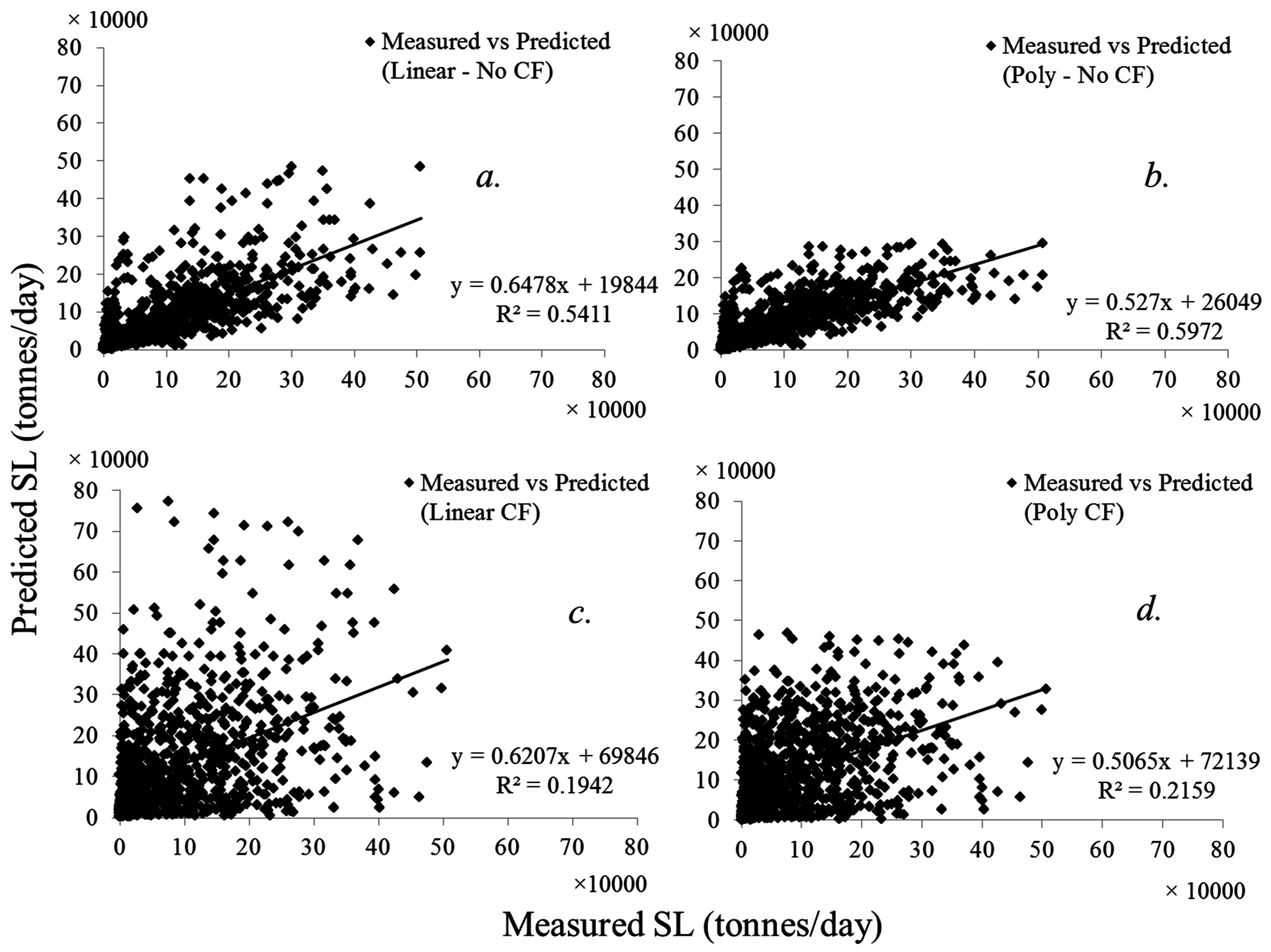
Single linear and polynomial rating curves were applied for the whole period at first, however, all four criteria to evaluate rating curves approach were not met here: lower R² (0.69 for linear and 0.7 for polynomial rating curve) (Table 1), comparatively higher RMSE (71,067 for linear and 67,950 for polynomial rating curve) (Table 2), comparatively higher SE (0.823) (Table 2), and poor visual agreement between corresponding measured and predicted DSLs (Figure 2). Low sample size of sediment concentrations during each year stopped us from applying sand rating curves annually during 1973–2013. In addition, rating curves in decadal intervals can minimize year to year variability in sediment samples and give robust average-annual predictions over decadal periods (supplementary information in [36]). Therefore, linear and polynomial rating curves were further applied for the following approximately decadal intervals in continuum: 1973–1985 (n = 463), 1986–1995 (n = 242), 1996–2005 (n = 187), and 2006–2013 (n = 142). The prerequisite of R² ≥ 0.8 was met for three of the four periods (1973–85: linear R² = 0.8, polynomial R² = 0.84; 1996–2005: linear R² = 0.81, polynomial R² = 0.83; 2006–13: linear R² = 0.82, polynomial R² = 0.87) (Table 1), so corresponding rating curves for these periods were subjected to further evaluation using other three criteria. However, the period 1986–95 had R²s (R-squares) < 0.8 (0.57) for both rating curves (Table 1). Thus, each year was checked with annual linear and polynomial rating curves to find the years responsible for lowering the combined linear and polynomial R²s in this period (

Table A1. Annual discharge-sand load rating curves developed for Tarbert Landing of the LmMR specifically during the period 1986–1995.

Year	No of Samples (n)	Discharge—Sand Load Rating Curve	Model	R2
1986	27	y = 0.9057x + 0.684	Linear	0.14
		y = −0.8658x2 + 17.012x − 74.858	Polynomial	0.15
1987	23	y = 1.0772x − 1.3125	Linear	0.27
		y = 0.2148x2 − 2.9014x + 17.059	Polynomial	0.27
1988	21	y = 1.4869x − 4.955	Linear	0.51
		y = 0.0868x2 − 0.0875x + 0.5817	Polynomial	0.51
1989	23	y = 1.5635x − 6.1185	Linear	0.40
		y = −0.1272x2 + 3.9797x − 17.559	Polynomial	0.40
1990	24	y = 0.6572x + 4.4327	Linear	0.14
		y = 1.0228x2 − 19.059x + 99.171	Polynomial	0.16
1991	24	y = 2.9061x − 17.418	Linear	0.87
		y = 1.6022x2 + 33.368x − 161.5	Polynomial	0.92
1992	25	y = 2.6355x − 14.51	Linear	0.72
		y = 1.7706x2 − 30.732x + 142.46	Polynomial	0.77
1993	31	y = 1.9324x − 7.3808	Linear	0.69
		y = 0.037x2 + 1.2055x − 3.813	Polynomial	0.69
1994	23	y = 3.0803x − 19.08	Linear	0.84
		y = −1.6631x2 + 35.256x − 174.26	Polynomial	0.87
1995	21	y = 2.8179x − 17.115	Linear	0.82
		y = −1.6093x2 + 33.441x − 162.32	Polynomial	0.87

in Appendix). We found all R²s during 1986–1990 (0.15–0.51) in one cluster, substantially lower than all R²s during 1991–1995 (0.69–0.92) in another cluster. Hence, based on approximation of individual R²s of annual rating curves, we combined the two periods 1986–90 (n = 118) and 1991–95 (n = 124) for further evaluation of their corresponding rating curves.

Table 1. Discharge-sand load rating curves developed for Tarbert Landing of the Lowermost Mississippi River (LmMR). Here, x = ln daily discharge (Q_d) (the independent variable) and y = ln daily sand load (DSL) (the dependent variable).

Period	Discharge—Sand Load Rating Curve	Model	R2
1973–2013	y = 2.2046x − 10.394	Linear	0.69
	y = −0.4685x2 + 11.091x − 52.388	Polynomial	0.70
1973–1985	y = 2.1964x − 10.214	Linear	0.80
	y = −0.6865x2 + 15.312x − 72.613	Polynomial	0.84
1986–1995	y = 2.3031x − 11.947	Linear	0.57
	y = 0.1371x2 − 0.274x + 0.1185	Polynomial	0.57
1986–1990	y = 1.4283x − 4.2019	Linear	0.36
	y = −0.1473 x2 + 4.1608x − 16.823	Polynomial	0.36
1991–1995	y = 2.8142x − 16.427	Linear	0.83
	y = −0.5842x2 + 13.993x − 69.687	Polynomial	0.86
1996–2005	y = 2.0516x − 8.7022	Linear	0.81
	y = −0.4666x2 + 10.9x − 50.514	Polynomial	0.83
2006–2013	y = 2.2267x − 10.204	Linear	0.82
	y = −0.6382x2 + 14.3x − 67.139	Polynomial	0.87

Table 1. Discharge-sand load rating curves developed for Tarbert Landing of the Lowermost Mississippi River (LmMR). Here, x = ln daily discharge (Q_d) (the independent variable) and y = ln daily sand load (DSL) (the dependent variable).

Period	Discharge—Sand Load Rating Curve	Model	R2
1973–2013	y = 2.2046x − 10.394	Linear	0.69
	y = −0.4685x2 + 11.091x − 52.388	Polynomial	0.70
1973–1985	y = 2.1964x − 10.214	Linear	0.80
	y = −0.6865x2 + 15.312x − 72.613	Polynomial	0.84
1986–1995	y = 2.3031x − 11.947	Linear	0.57
	y = 0.1371x2 − 0.274x + 0.1185	Polynomial	0.57
1986–1990	y = 1.4283x − 4.2019	Linear	0.36
	y = −0.1473 x2 + 4.1608x − 16.823	Polynomial	0.36
1991–1995	y = 2.8142x − 16.427	Linear	0.83
	y = −0.5842x2 + 13.993x − 69.687	Polynomial	0.86
1996–2005	y = 2.0516x − 8.7022	Linear	0.81
	y = −0.4666x2 + 10.9x − 50.514	Polynomial	0.83
2006–2013	y = 2.2267x − 10.204	Linear	0.82
	y = −0.6382x2 + 14.3x − 67.139	Polynomial	0.87

Table 2. Root mean square errors (RMSEs) of DSLs predicted through discharge-sand load rating curves for each period in Table 1. Here, SE is the standard error and CF-Poly is the Duan correction factor used in polynomial rating curves, while CF-Lin is the Duan correction factor used in linear rating curves. “No CF” represents DSLs calculated without applying correction factors during their retransformation from predicted ln DSLs while “CF” represents DSLs calculated by applying the correction factors during the retransformation procedure.

Period	RMSE-No CF (Polynomial)	RMSE-No CF (Linear)	SE	CF-Poly	CF-Lin	RMSE-CF (Polynomial)	RMSE-CF (Linear)
1973–2013	67,950	71,067	0.823	1.586	1.592	75,091	98,817
1973–1985	61,604	72,892	0.596	1.194	1.213	62,099	85,875
1986–1990	41,021	41,248	1.132	1.841	1.662	181,902	129,574
1991–1995	62,625	71,692	0.572	1.141	1.174	63,491	81,031
1996–2005	48,444	55,213	0.505	1.155	1.152	48,899	61,483
2006–2013	50,261	81,456	0.496	1.122	1.13	51,409	94,689

Table 2. Root mean square errors (RMSEs) of DSLs predicted through discharge-sand load rating curves for each period in Table 1. Here, SE is the standard error and CF-Poly is the Duan correction factor used in polynomial rating curves, while CF-Lin is the Duan correction factor used in linear rating curves. “No CF” represents DSLs calculated without applying correction factors during their retransformation from predicted ln DSLs while “CF” represents DSLs calculated by applying the correction factors during the retransformation procedure.

Period	RMSE-No CF (Polynomial)	RMSE-No CF (Linear)	SE	CF-Poly	CF-Lin	RMSE-CF (Polynomial)	RMSE-CF (Linear)
1973–2013	67,950	71,067	0.823	1.586	1.592	75,091	98,817
1973–1985	61,604	72,892	0.596	1.194	1.213	62,099	85,875
1986–1990	41,021	41,248	1.132	1.841	1.662	181,902	129,574
1991–1995	62,625	71,692	0.572	1.141	1.174	63,491	81,031
1996–2005	48,444	55,213	0.505	1.155	1.152	48,899	61,483
2006–2013	50,261	81,456	0.496	1.122	1.13	51,409	94,689

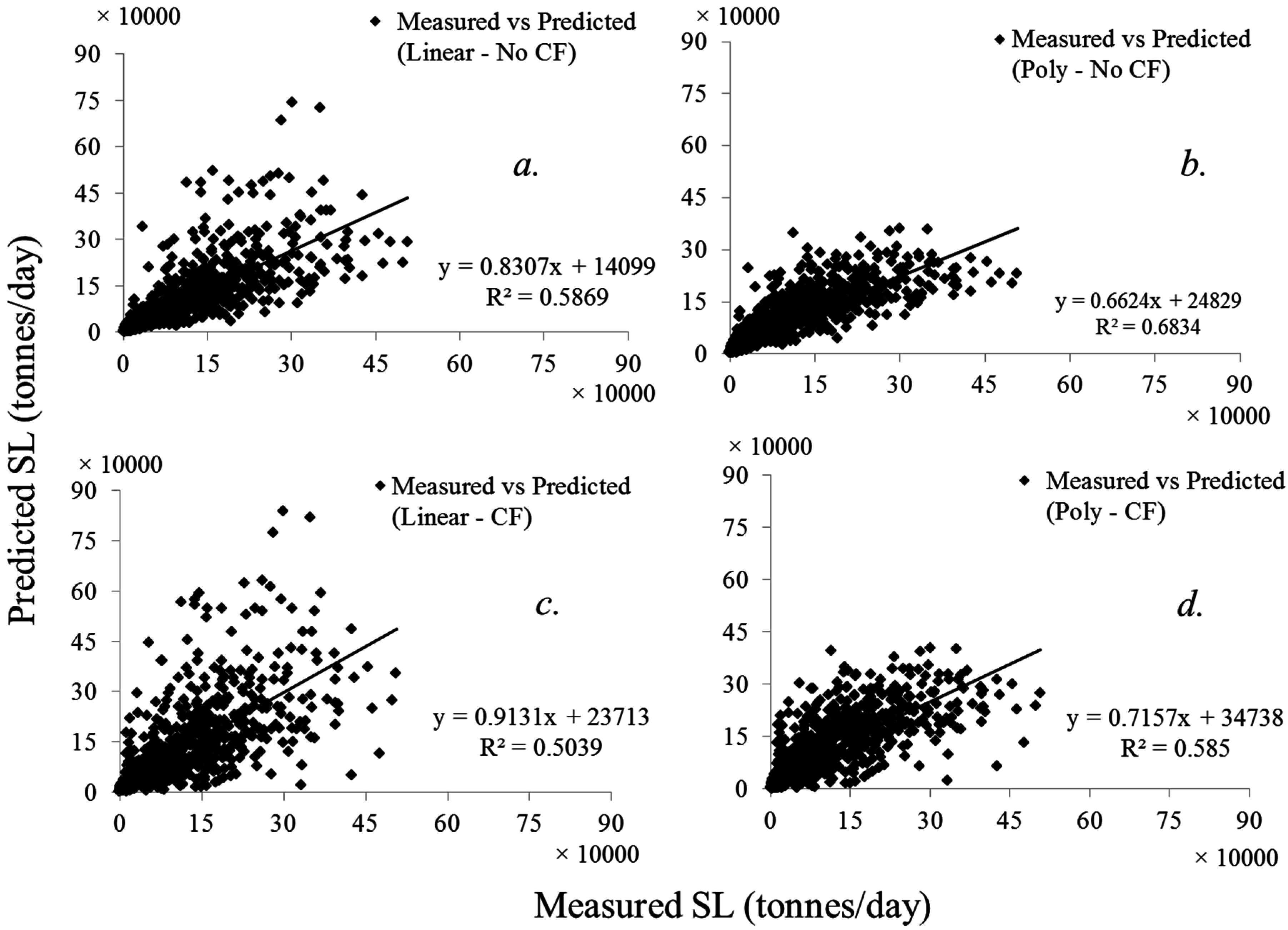
Finally, we found that polynomial discharge-sand load rating curves during the four durations: 1973–1985, 1991–1995, 1996–2005 and 2006–2013 met all the four criteria and provided DSL estimates most approximate to the measured DSLs (Table 1 and Table 2; Figure 3). We also found that the use of correction factors overestimated DSLs slightly (for polynomial curves) as well as substantially (for linear curves) as compared to their corresponding calibrated measurements (Table 2; Figure 2 and Figure 3). Hence, based on evaluation of these overestimations and previous arguments regarding unreliability of the correction factors [49,50], we decided to use polynomial sand rating curves categorized into aforementioned four periods without correction factor to calculate sand loads for each day from 1973 to 2013 except for the period 1986–1990. The reason for excluding rating curve analysis from 1986 to 1990 and the procedure followed to calculate daily sand loads during this period have been explained in Section 2.6 further down.

Figure 2. Scatter plots showing comparison between sand loads calculated from sand concentrations measured, processed and calibrated by USGS (Measured SL) and those predicted from single sand-rating curve (either linear or polynomial) (Predicted SL) at Tarbert Landing from 1973 to 2013. Here, linear rating curves were used for predicting SLs in (a) and (c)while polynomial rating curves were used for predicting SLs in (b) and (d). In addition, Duan correction factors were applied in predicted SLs of curves (c) and (d) (denoted by “CF” in the figure) while the SLs in curves (a) and (b) were predicted without correction factors (denoted by “No CF” in the figure).

Figure 2. Scatter plots showing comparison between sand loads calculated from sand concentrations measured, processed and calibrated by USGS (Measured SL) and those predicted from single sand-rating curve (either linear or polynomial) (Predicted SL) at Tarbert Landing from 1973 to 2013. Here, linear rating curves were used for predicting SLs in (a) and (c)while polynomial rating curves were used for predicting SLs in (b) and (d). In addition, Duan correction factors were applied in predicted SLs of curves (c) and (d) (denoted by “CF” in the figure) while the SLs in curves (a) and (b) were predicted without correction factors (denoted by “No CF” in the figure).

Figure 3. Scatter plots showing comparison between sand loads calculated from sand concentrations measured, processed and calibrated by USGS (Measured SL) and those predicted from several sand-rating curves (Predicted SL) at Tarbert Landing from 1973 to 2013. Specific terminologies pertaining to parts (a), (b), (c) and (d) of this figure i.e., Linear, Poly, CF, and No CF are same as explained in Figure 2. It is noted that both predicted and measured SLs during the period 1986–1990 were eliminated in this comparison because of the low R² value of both rating curves during this period (please see Table 1).

Figure 3. Scatter plots showing comparison between sand loads calculated from sand concentrations measured, processed and calibrated by USGS (Measured SL) and those predicted from several sand-rating curves (Predicted SL) at Tarbert Landing from 1973 to 2013. Specific terminologies pertaining to parts (a), (b), (c) and (d) of this figure i.e., Linear, Poly, CF, and No CF are same as explained in Figure 2. It is noted that both predicted and measured SLs during the period 1986–1990 were eliminated in this comparison because of the low R² value of both rating curves during this period (please see Table 1).

2.6. Non-Rating Curve Approach for Sand Load Calculation

For the period of 1986–1990, three of the four criteria to evaluate rating curves approach were not met: lower R² (0.36 for both polynomial and linear rating curves) (Table 1), comparatively higher SE (1.132) (Table 2) and poor visual agreement between corresponding measured and predicted DSLs (Figure 4). Therefore, calibrated sand concentration measurements (117 samples) and daily discharge were used to calculate sand loads for each day during this period. Here, starting from 1986, the earliest available sand concentration of the year was assumed to be equal to all consecutive days of missing concentration until the next value was available. In addition, last available concentration of the earlier year was used for filling values of missing days of the current year if the earliest concentrations did not start from the first day of the year. Finally, DSLs for non-sand rating curve years were calculated using the formula in Equation (1).

Figure 4. Scatter plots showing comparison between sand loads calculated from sand concentrations measured, processed and calibrated by USGS (Measured SL) and those predicted from single sand-rating curve (either linear or polynomial) (Predicted SL) at Tarbert Landing from 1986 to 1990. Specific terminologies pertaining to parts (a), (b), (c) and (d) of this figure i.e., Linear, Poly, CF, and No CF are same as explained in Figure 2.

Figure 4. Scatter plots showing comparison between sand loads calculated from sand concentrations measured, processed and calibrated by USGS (Measured SL) and those predicted from single sand-rating curve (either linear or polynomial) (Predicted SL) at Tarbert Landing from 1986 to 1990. Specific terminologies pertaining to parts (a), (b), (c) and (d) of this figure i.e., Linear, Poly, CF, and No CF are same as explained in Figure 2.

2.7. Range of Errors Associated with Predicted Sand Loads

We considered two types of errors (E-1 and E-2) in the SL estimates (it must be noted that the standard errors discussed earlier in Section 2.5 accounted for the entire models rather than individual estimates). E-1 is associated with the methods used by USGS for depth-integrated sampling and calibration of SSCs. It has previously been reported to be approximately ±10% of the total calibrated SSCs, SSC_ss and SSC_fs [51,52,53]. E-2 is associated with dependent variables (ln SL) in the rating curves. The confidence intervals (CI) for each “ln predicted SL” at 95% level of significance in their rating curves were provided with the help of their corresponding E-2s in our analysis (Figure 5). We estimated an approximate E-2 of ±15% in all SLs predicted from rating curve approach (based on confidence interval plots, RMSEs and percentage difference between measured and predicted SLs which averaged −13.4% during the four periods). Thus, the total error in SL measurements and predictions (E-1 + E-2) during rating curve years was about ±25%. We only selected E-1 for all estimates during 1986–1990 because we did not use rating curve approach in this period. Therefore, error range for SL estimates during 1986–1990 was ±10%. For convenience and consistency in reporting, we used an error range of ±18% for all the SL estimates during 1973–2013 (approximately ~average of 25 and 10).

Figure 5. Confidence interval (CI) for the all “ln predicted SL” values at 95% confidence level in accordance to their corresponding SSC_s-Q_d rating curves during the four periods as shown at Tarbert Landing. It is noted that in all four periods (a), (b), (c) and (d), uppermost and lowermost curves represent the upper and lower limits of the CI, while the middle curve represents all individual “ln predicted SL” values as given in a.

Figure 5. Confidence interval (CI) for the all “ln predicted SL” values at 95% confidence level in accordance to their corresponding SSC_s-Q_d rating curves during the four periods as shown at Tarbert Landing. It is noted that in all four periods (a), (b), (c) and (d), uppermost and lowermost curves represent the upper and lower limits of the CI, while the middle curve represents all individual “ln predicted SL” values as given in a.

2.8. Daily, Annual and Seasonal Sand Load Trends

DSLs were calculated using aforementioned methods of rating curve (1973–1985, 1991–1995, 1996–2005, 2006–2013) and non-rating curve (1986–1990) approaches. The sum of DSLs from 1st January to 31st December during each year gave their corresponding annual SLs. Maximum, minimum and average DSLs and annual SLs were plotted against their corresponding years for information regarding daily and annual SL trends throughout the study period. Similarly, monthly SLs were calculated by averaging DSLs for each month separately from 1973 to 2013. Maximum, minimum and average monthly SLs were plotted against their corresponding months to analyze their seasonal trends.

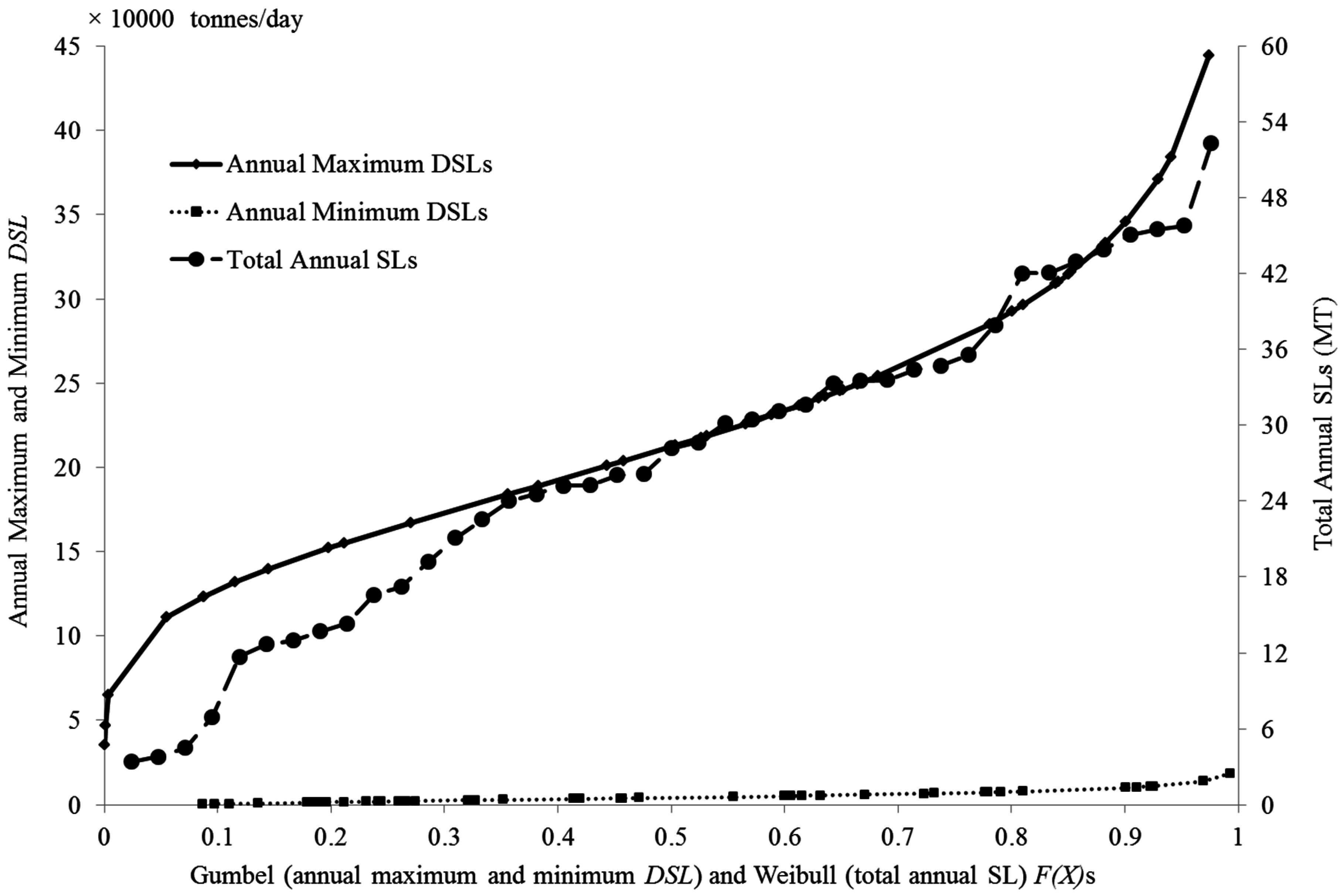
2.9. Frequency Analysis of Sand Loads

In this study, we analyzed the amount of sand transported at Tarbert Landing during 1973–2013 under different river flow conditions, i.e., six frequencies on the flow duration curves (1%, 5%, 10%, 20%, 50%, and 75%) and five river stages (Low, Action, Intermediate, High, and Peak). The Gumbel distribution [54,55] was used for analyzing annual maximum and minimum DSLs, while the Weibull distribution [56,57] was used for analyzing total annual sand loads (SL) at Tarbert Landing. All annual maximum/minimum DSLs and total annual SLs during 1973 and 2013 were sorted in descending order separately at first. The non-exceedance probabilities {F(X)} for maximum and minimum DSLs were obtained with the Gumbel distribution (Equation (3)), while the non-exceedance probabilities for total annual SLs were obtained with the Weibull distribution (Equation (4)) as given below:

$$GumbelF\left(X\right)=e^{-e^{-\left(\frac{X-a}{b}\right)}}$$

(3)

$$WeibullF\left(X\right)=1-\frac{m}{n+1}$$

(4)

where X is annual maximum/minimum DSL (tonnes/day) or total annual SL (megatonnes), m is the rank of the annual SL, n is the total number of years in the distribution, and a and b are the Gumbel distribution parameters that were calculated through:

$$a={\mu }_x-0.5772b$$

(5)

$$b=\frac{S_x\sqrt{6}}{\pi }$$

(6)

where µ_x is the average and S_x is the standard deviation of the annual maximum and minimum DSLs.

Maximum and minimum DSLs (Q_p) for the return periods [T(X)] of 2-, 5-, 10-, 20-, and 40-years were calculated using the Gumbel distribution as:

$$Q_p=K\left(T\right)S_x$$

(7)

where the frequency factor K(T) is defined as:

$$K\left(T\right)=-\frac{\sqrt{6}}{\pi }\left\{0.5772+LnLn\left[\frac{T\left(X\right)}{T\left(X\right)-1}\right]\right\}$$

(8)

A frequency factor is computed for a certain return. In this study, we computed frequency factors of −0.1643, 0.7195, 1.3046, 1.8658, and 2.4163 for the 2-, 5-, 10-, 20-, and 40-year return periods, respectively. Annual SLs for the same return periods were estimated using a linear interpolation from the Weibull distribution of annual SLs (i.e., 1/{1–F(X)}).

3. Results

3.1. Long-Term River Flow Conditions

Daily discharge (Q_d) at Tarbert Landing from 1973 to 2013 averaged 15,027 cms, varying from 3143 to 45,844 cms (Figure 6). During this period, average Q_d was lowest in 2000 (9558 cms) and highest in 1993 (21,844 cms). Similarly, average Q_d fell within the Low flow stage (<13,000 cms) for 11 years (1976, 1977, 1980, 1981, 1987, 1988, 2000, 2005, 2006, 2007 and 2012), Intermediate flow stage (18,000–25,000 cms) for seven years (1973, 1979, 1983, 1991, 1993, 2008 and 2009), and Action flow stage (13,000–18,000 cms) for the remaining 23 years (Figure 6). In addition, years with higher average Q_ds had higher minimum and maximum Q_ds as compared to years with lower average daily Q_ds (Figure 6). Additionally, Low, Action, Intermediate, High and Peak flow stages accounted for about 50%, 17%, 21%, 9% and 3% of all the discharge events throughout the study period, respectively (Figure 7, Table 3). In addition, 1%, 5%, 10, 20%, 50% and 75% flows corresponded to the flow intervals of 37,943–45,844, 26,931–45,844, 22,256–45,844, 13,082–45,844 and 8325–45,844 cms, respectively (Figure 7).

Seasonally, average Q_d increased continuously from January to its maximum in April (16,550 to 22,468 cms), then decreased continuously from May to its minimum in October (21,696 to 8171 cms) inferring maximum river flow during the spring months (March, April and May) (Figure 8). For the remaining two months in the year, average Q_d followed an increasing trend again (9702 cms in November and 14,581 cms in December) (Figure 8). In addition, the maximum Q_d was observed in May (45,844 cms) while the minimum Q_d was observed in July (3143 cms) (Figure 8).

Figure 6. Annual mean, maximum, and minimum of daily discharge at Tarbert Landing of the LmMR.

Figure 6. Annual mean, maximum, and minimum of daily discharge at Tarbert Landing of the LmMR.

Figure 7. Flow duration curve for Tarbert Landing of the LmMR during 1973–2013. The vertical dash lines represent the exceedance probabilities for five river stages as defined by NOAA, i.e., Peak, High, Intermediate, Action and Low Flow Stages.

Figure 7. Flow duration curve for Tarbert Landing of the LmMR during 1973–2013. The vertical dash lines represent the exceedance probabilities for five river stages as defined by NOAA, i.e., Peak, High, Intermediate, Action and Low Flow Stages.

Figure 8. Seasonal trend of monthly mean, maximum, and minimum of daily discharge at Tarbert Landing of the LmMR during 1973–2013.

Figure 8. Seasonal trend of monthly mean, maximum, and minimum of daily discharge at Tarbert Landing of the LmMR during 1973–2013.

Table 3. Long-term flow conditions based on the U.S. National Oceanic and Atmospheric Administration (NOAA’s) Mississippi River flow stages at Tarbert Landing of the LmMR from 1973 to 2013.

Flow Stage (m)	Discharge Range (cms) *	Occurrence (%)
Low (<9.8)	<13,000	49.70
Action (9.8–12.1)	13,000–18,000	16.82
Intermediate (12.1–14.6)	18,000–25,000	20.74
High (14.6–16.8)	25,000–32,000	9.33
Peak (>16.8)	>32,000	3.41

Note: * The discharge ranges for Intermediate, High, and Peak Flow Stages are adopted from Rosen and Xu [21].

Table 3. Long-term flow conditions based on the U.S. National Oceanic and Atmospheric Administration (NOAA’s) Mississippi River flow stages at Tarbert Landing of the LmMR from 1973 to 2013.

Flow Stage (m)	Discharge Range (cms) *	Occurrence (%)
Low (<9.8)	<13,000	49.70
Action (9.8–12.1)	13,000–18,000	16.82
Intermediate (12.1–14.6)	18,000–25,000	20.74
High (14.6–16.8)	25,000–32,000	9.33
Peak (>16.8)	>32,000	3.41

Note: * The discharge ranges for Intermediate, High, and Peak Flow Stages are adopted from Rosen and Xu [21].

3.2. Sand Concentrations under Different Flow Regimes

Average SSC_ss and their percentage changes at Tarbert Landing showed early increasing trend from the lowest Q_d interval (3000–6000 cms) (Figure 9). Average SSC_s for the lowest Q_d interval (3000–6000 cms) was about 11 mg/L which increased up to about 91 mg/L between 24,000 and 27,000 cms Q_d (715% increase) (Figure 9). Further, average SSC_ss fluctuated for higher Q_d intervals, i.e., they first decreased up to approximately 70 mg/L for Q_d interval between 30,000 and 36,000 cms (715% to 529%), then increased up to approximately 103 mg/L for the next interval between 36,000 and 39,000 cms (529% to 832%), then decreased up to about 72 mg/L (832% to 552%) for the next interval between 39,000 and 42,000 cms and finally increased up to about 82 mg/L (552% to 642%) for the highest Q_d interval (42,000–45,000 cms) (Figure 9). Similar trends were also observed in individual SSC_s values across the entire Q_d range. SSC_ss showed an early increasing trend even with lower discharge levels (about 6000 cms) which continued until substantially high flows (27,000 cms with R² = 0.36) (Figure 10). The elevated concentrations remained almost constant (R² = 0.0061) for higher flows (>27,000 cms) (Figure 10).

Figure 9. Average sand concentrations and percentage change with each 3000 cms increment of discharge at Tarbert Landing of the LmMR during 1973–2013.

Figure 9. Average sand concentrations and percentage change with each 3000 cms increment of discharge at Tarbert Landing of the LmMR during 1973–2013.

Figure 10. Distribution of sand concentration with discharge at Tarbert Landing of the LmMR during 1973–2013.

Figure 10. Distribution of sand concentration with discharge at Tarbert Landing of the LmMR during 1973–2013.

3.3. Daily, Annual and Seasonal Trend of Sand Loads

Daily Sand Loads at Tarbert Landing from 1973 to 2013 averaged 74,474 tons, varying from 258 to 44,4626 tons (Figure 11). During this period, average DSL was lowest in 1987 (9300 tons/day) and highest in 1993 (143,322 tons/day) (Figure 11). Average DSL was lower than 20,000 tons for 4 years (1986, 1987, 1988 and 1989), higher than 100,000 tons for 9 years (1973, 1979, 1983, 1991, 1993, 2008, 2009, 2010 and 2011), and either >20,000 or <100,000 tons for the remaining 28 years (Figure 11). As with average Q_d, years with higher average DSLs had higher minimum and maximum DSLs as compared to years with lower average DSLs (Figure 11).

Annual sand load from 1973 to 2013 averaged 27.2 MT, ranging from 3.37 to 52.30 MT and producing a total sand amount of 1114.82 MT for the entire 41-year study period (Figure 11). Annual SL was lower than 10 MT for four of 41 years (1986, 1987, 1988 and 1989), higher than 40 MT for eight years including the Mississippi flood years of 1973, 1993 and 2011, and either > 10 MT or < 40 MT for the remaining 29 years (Figure 11). In addition, annual SL averaged 26.3 MT from 1973 to 1999 (28.8 MT from 1972 to 1979, 19.3 MT from 1980 to 1989, 32 MT from 1990 to 1999), which later increased to approximately 29 MT from 2000 to 2013 (calculations from table of Figure 11). Despite the low average annual SL between 1986 and 1989, there was no continuous increasing or decreasing trend (even for 2/3 years) in annual SL (Figure 11).

Figure 11. Annual mean, maximum, and minimum of daily sand loads and total annual sand loads at Tarbert Landing of the LmMR.

Figure 11. Annual mean, maximum, and minimum of daily sand loads and total annual sand loads at Tarbert Landing of the LmMR.

Seasonal trend of the average DSL was similar to that of the average Q_d. Average DSL increased continuously from January to its maximum in May (i.e., 86,315 to 137,387 tons/day), then decreased from June to its minimum in September (106,426 to 14,935 tons/day) inferring maximum sand transport during spring (March, April and May) (Figure 12). For the remaining three months in the year, average DSL followed an increasing trend again, i.e., 20,871 tons/day in October to 70,092 tons/day in December (Figure 12). In addition, maximum DSL was observed in June (444,626 tons/day) while minimum DSL was observed in August (258 tons/day) for the whole period (Figure 12).

3.4. Sand Load Distribution with River Discharge

Hydrologically, with respect to the NOAA’s river stages, Intermediate, High and Peak Flow Stages together carried majority of the total SL (793.4 MT; 71%) within an average of 122 days per year (Table 4). Individually, Intermediate, High and Peak Flow Stages carried approximately 384 (34%), 266 (24%) and 143 (13%) MT of SLs for average durations of 76, 34 and 12 days/year respectively, while, Low and Action Flow Stages carried approximately 146 (13%) and 175 (16%) MT of SL respectively for relatively longer average durations of 181 and 61 days/year (Table 4). Also, 50% and 75% of flow regimes produced majority of total SL in the area, i.e., 966 (87%) and 1082 MT (97%) respectively (Table 5). Similarly, 1%, 5%, 10% and 20% of flow regimes also produced few to slightly more than half of total SL, i.e., 46 (4%), 196 (18%), 340 (31%) and 571 MT (51%), respectively (Table 5).

Figure 12. Seasonal trend of monthly mean, maximum, and minimum of daily sand load at Tarbert Landing of the LmMR during 1973–2013.

Figure 12. Seasonal trend of monthly mean, maximum, and minimum of daily sand load at Tarbert Landing of the LmMR during 1973–2013.

Table 4. Sand transport under five river stages at Tarbert Landing of the LmMR from 1973 to 2013.

Flow Stage	Sand Load (MT)	% of Total SL (1114.8 MT)	Total # of Days	Average No. of Days/Year
Low	146.24	13.12	7440	181
Action	174.89	15.69	2518	61
Intermediate	384.26	34.47	3104	76
High	266.15	23.87	1397	34
Peak	143.00	12.85	510	12

Table 4. Sand transport under five river stages at Tarbert Landing of the LmMR from 1973 to 2013.

Flow Stage	Sand Load (MT)	% of Total SL (1114.8 MT)	Total # of Days	Average No. of Days/Year
Low	146.24	13.12	7440	181
Action	174.89	15.69	2518	61
Intermediate	384.26	34.47	3104	76
High	266.15	23.87	1397	34
Peak	143.00	12.85	510	12

Table 5. Sand transport within 1%, 5%, 10%, 20%, 50%, and 75% flow regimes at Tarbert Landing of the LmMR from 1973 to 2013.

Total Sand Load (MT)	Sand Load (MT) in Flow Regimes
	1%	5%	10%	20%	50%	75%
1114.80	45.63	196.21	340.18	571.36	966.40	1082.50
% of total SL	4.09	17.60	30.51	51.25	86.69	97.10

Table 5. Sand transport within 1%, 5%, 10%, 20%, 50%, and 75% flow regimes at Tarbert Landing of the LmMR from 1973 to 2013.

Total Sand Load (MT)	Sand Load (MT) in Flow Regimes
	1%	5%	10%	20%	50%	75%
1114.80	45.63	196.21	340.18	571.36	966.40	1082.50
% of total SL	4.09	17.60	30.51	51.25	86.69	97.10

Linear relationship between all annual flow volumes (km³) above the low and action flow stages (discharge ≥ 18,000 cms) and corresponding annual sand loads (MT) showed that intermediate, high and peak flow stages jointly accounted for about 66% variation in sand loads during each year from 1973 to 2013 (R² = 0.66) (Figure 13). The relationship further suggested that about 66% of sand loads were produced by these three stages jointly during each year of the study period.

Figure 13. Annual flow volume above the Low and Action flow stages (discharge ≥ 18,000 cms) versus annual sand load at Tabert Landing of the LmMR during 1973–2013.

Figure 13. Annual flow volume above the Low and Action flow stages (discharge ≥ 18,000 cms) versus annual sand load at Tabert Landing of the LmMR during 1973–2013.

3.5. Maximum and Minimum Sand Loads for Different Return Periods

Averages of maximum and minimum DSLs for each year throughout the whole study period at Tarbert Landing were 226,981 and 4865 tonnes/day, while their standard deviations were 90,595 and 4015 tonnes/day respectively (Table 6). Based on these means and standard deviations, parameters a and b in Gumbel distribution were found to be 186,209 and 70,637 for highest DSLs and 3058 and 3131 for lowest DSLs during each year respectively (Table 6).

Table 6. Mean (µ_x), Standard Deviations (SD) (S_x) and respective parameters (a and b) in Gumbel distribution for maximum and minimum DSL (tonnes/day) at Tarbert Landing of the LmMR from 1973 to 2013.

Distributions	Mean and SD	Gumbel Parameters	Value
Maximum DSL	${\mu }_x$ = 226981	a	186209
	Sx = 90595	b	70637
Minimum DSL	${\mu }_x$ = 4865	a	3058
	Sx = 4015	b	3131

Table 6. Mean (µ_x), Standard Deviations (SD) (S_x) and respective parameters (a and b) in Gumbel distribution for maximum and minimum DSL (tonnes/day) at Tarbert Landing of the LmMR from 1973 to 2013.

Distributions	Mean and SD	Gumbel Parameters	Value
Maximum DSL	${\mu }_x$ = 226981	a	186209
	Sx = 90595	b	70637
Minimum DSL	${\mu }_x$ = 4865	a	3058
	Sx = 4015	b	3131

Non-exceedance probabilities of maximum and minimum DSLs {Gumbel F(X)} and total SLs {Weibull F(X)} for each year from 1973 to 2013 are represented by Figure 14. For longer return periods of 20 and 40 years, we predicted that DSLs at Tarbert Landing can reach a maximum of 396 and 446 thousand tons and a minimum of 12 and 15 thousand tons, respectively (Table 7). Similarly, for shorter return periods of 2, 5, and 10 years, maximum DSL predictions were 212, 292, and 345 thousand tons respectively, while minimum DSL predictions were 4, 8, and 10 thousand tons, respectively (Table 7). We also predicted that in the next 2-, 5-, 10-, 20-, and 40-years total annual sand load can reach as much as 28.2, 40.28, 44.78, 45.76 and 51.68 MT, respectively (Table 7).

Figure 14. Non-exceedance probabilities of the Gumbel distribution for maximum and minimum DSLs and Weibull distribution for total SLs each year at Tarbert Landing of the LmMR from 1973 to 2013.

Figure 14. Non-exceedance probabilities of the Gumbel distribution for maximum and minimum DSLs and Weibull distribution for total SLs each year at Tarbert Landing of the LmMR from 1973 to 2013.

Table 7. Gumbel distribution based prediction of maximum and minimum DSLs and Weibull distribution based prediction of total annual SLs for the 2-, 5-, 10-, 20-, and 40-year returns at Tarbert Landing of the LmMR.

Return Period (Years)	Extreme Sand Loads
	Annual SL (MT/Year)	Maximum DSL (x 1000 Tonnes/Day)	Minimum DSL (x 1000 Tonnes/Day)
2	28.20	212	4
5	40.28	292	8
10	44.78	345	10
20	45.76	396	12
40	51.68	446	15

Table 7. Gumbel distribution based prediction of maximum and minimum DSLs and Weibull distribution based prediction of total annual SLs for the 2-, 5-, 10-, 20-, and 40-year returns at Tarbert Landing of the LmMR.

Return Period (Years)	Extreme Sand Loads
	Annual SL (MT/Year)	Maximum DSL (x 1000 Tonnes/Day)	Minimum DSL (x 1000 Tonnes/Day)
2	28.20	212	4
5	40.28	292	8
10	44.78	345	10
20	45.76	396	12
40	51.68	446	15

4. Discussion

4.1. Long-Term Trend of Sand Loads in the LmMR

In this study we present sand transport estimates for each individual year along with their error range (±18%), providing a comprehensive range of sand transport in the past four decades. Previously, Nittrouer and Viraparelli [36] reported an average annual sand transport of about 24 MT for Tarbert Landing during 1973 and 2012, which is about 12% lower than our estimate for average annual sand transport (27 ± 4.9 MT) during 1973 and 2013. This difference falls within the total error range of all SL estimates in this study (±18%). The relatively small difference between the two estimates may be caused by different estimation approaches: Nittrouer and Viraparelli used linear rating curves at decadal intervals for daily sand load estimation while this study used a combination of five-yearly to approximately decadal polynomial rating curves and monthly sand concentration records. Our SL estimate for 2013 (31 ± 5.6 MT), which was not included in Nittrouer and Viraparelli’s analysis, was about 14% higher than our 41-year long average SL estimate; however, this difference also falls within our error range (±18%).

In their short-term sediment budget study, Allison et al. [30] reported an annual SL of 73.5, 62.2 and 78.9 MT for the water years of 2008, 2009 and 2010, respectively, resulting in a total SL of 214.6 MT. These estimates are 62%, 36% and 108% higher than our calendar-based estimates for these three years (45.5 ± 8.1, 45.8 ± 8.2 and 38.0 ± 6.8 MT, respectively), or nearly doubled of our estimate for the entire three years (129.3 ± 23.3 MT). These two sets of estimates cannot be compared directly because of the different time base; however, it seems that Allison et al. [30] overestimated annual SLs for 2008, 2009 and 2010 water years at Tarbert Landing. Allison et al.’s SL estimates for 2008, 2009 and 2010, respectively, were numerically higher than 38, 36 and 42 of 45 annual SL estimates provided by USACE for all water years from 1952 to 1996 [58]. In addition, the rating curve which Allison et al. [30] used to calculate DSLs for each day during the three years had a comparatively lower R² (0.62) (information from the supplementary files of Allison et al. [30]) and no other criteria for model validation which could have resulted in greater variability between calibrated and estimated SLs. Furthermore, their estimates do not fall within the error range of our annual estimates during these three years. These three arguments provide essential support for questioning the reliability of their estimates.

In our study, we found a very low sand transport during 1986 and 1989. Only 19 ± 1.9 MT of sand was discharged during this four-year period, making an average annual SL of just 5 MT, i.e., less than one fifth of the long-term average annual SL of 27 ± 4.9 MT. Nittrouer and Viraparelli [36] also reported low average SL for a period longer than these four years (1980 to 1989) (about 11 MT); however, they did not separate SLs for each year during the four-year period. The notable abrupt drop in sand transport during these four years may have been a result from the four-year severe drought in the Southeastern and Midwestern United States between 1986 and 1989, as reported by Cook et al. [59] and Trenberth and Guillemot [60]. During this drought period, both discharge and sediment concentrations of the LmMR were considerably lower than those of other years in the past four decades.

The declining trend of total suspended sediment load input in the LmMR during the last several decades has been well documented [6,61,62,63]. However, Rosen and Xu [21] contradicted this trend by suggesting that suspended sediment input has slightly increased in the river for the recent two decades (from 1990 to 2010), although no statistical significance was found. Our findings for sand transport (the courser sediment fraction) are identical with Rosen and Xu [21] as we also found a stronger increasing trend in sand loads starting from 1990—the average annual sand load from 1990 to 2013 (30 ± 5.4 MT) was clearly higher than that during 1973 and 1989 (23 ± 4.1 MT). The higher sand transport in the past two decades has mainly resulted from the increased discharge during the same period of time.

4.2. Hydrologic Control for Sand Transport in the LmMR

Our findings suggest that notable sand load present in the LmMR can best be diverted during its intermediate, high and peak flow stages (discharge ≥ 18,000 cms) within only approximately four months each year. We found that maximum river flow and sand transport both occurred during the spring months (March, April and May); therefore, it is highly likely that the three river stages are prevalent during spring and scarce during other seasons of the year. Highest sand transport by these three stages can be linked to their rapid increase in discharge regimes from nearly 6000 to 27,000 cms and very slow and inconsistent decrease in regimes post 27,000 cms. Sand concentrations seem to have reached their peaks during the intermediate and early high flow stages (discharge: 18,000–27,000 cms), hence resulting in the highest sand loads.

There is no previous work available for comparison to these findings of long term sand load availability with river discharge. The work by Rosen and Xu [21] seems to support our findings, but they analyzed the availability of total suspended sediments with river discharge as compared to the total sand load in our study and emphasized that intermediate and high river stages combined carry highest sediment loads, however, peak stage contributes relatively little in sand transport. Biedenharn and Thorne [64] argued that discharge between 17,000 and 40,000 cms transport more suspended sediments than other discharge regimes. Differences in weights and volumes of sediment and sand concentrations may be the reason behind subtle differences in flow regimes reported to carry highest sediment and sand loads in these studies. We also found that almost the entire total sand load (97%) in the LmMR was transported by 75% of total water discharge throughout the study period. This discharge regime includes almost half of the lower flow stage along with all other Mississippi River stages (>8325 cms) at Tarbert Landing. The sand behaviors found in this study—(1) increasing rapidly with increasing discharge; however, decreasing slowly beyond a given discharge regime just after reaching its climax; and (2) maximum sand percentage transported by substantially less flow volume percentage—can be compared with other large river systems in the world with a sinking delta. Such information can help planning for deltaic land protection through effective sand management.

4.3. Future Likelihood of Sand Transport in the LmMR

Our frequency analysis reveals that the LmMR at Tarbert Landing has the potential to transport substantial amount of sand every day in the next 40 years (4 to 446 thousand tonnes). Based on the sand yields at different river stages, we argue that the intermediate, high and/or peak river stages will possibly transport higher DSLs in shorter periods while low and/or action stages will possibly transport lower DSLs in longer periods of time. Our findings further indicated that annual sand load has the potential to reach as much as 52 MT in the next 40 years. Based on our observations regarding the linear relationship between annual flow volumes in intermediate, high and peak flow stages and annual SLs, we also argue that years with high average daily discharge and annual flow would produce high annual sand loads within the given return periods and vice-versa. Previous studies have analyzed several year peaks for suspended sediment loads and concentrations [65,66] and even for river flows and stages [67,68] in different rivers around the world. However, to the best of our knowledge, maximum and minimum DSLs and annual SLs for short- and long-term return periods have not been analyzed for any river location to date. Thus, we could not compare these sand estimates in the LmMR with any other study.

The peak high and low DSLs and peak annual SLs vary between Tarbert Landing and other sites in the LmMR and the variation is based on sand-flow relationship and sand percentage in sediment load. Quantification of peak SLs at other sites is beyond the scope of this study. However, the analysis of daily and annual sand loads for several return periods can be helpful in speculating the importance of sediment diversion as per sand amount present at the site. It is also possible to incorporate the maximum/minimum DSLs and annual SLs for several return periods into any proposed land loss model for the MRDP. This can be done by quantifying the percentage loss of sand when given land area (km²) was lost in “n” (where n = 2, 5, 10, 20, or 40) years and/or the amount of sand required to attain a goal of restoring certain land (km²) in “n” years.

5. Conclusions

This study is the first comprehensive analysis of four-decade long sand transport under different flow conditions in the Lowermost Mississippi River. Our findings show that the majority of sand at Tarbert Landing are transported during the intermediate, high and peak river flow stages, and that their most effective capture can be achieved within 120 days of a year when discharge is greater than 18,000 cms. We also predict that the LmMR will most likely transport 4 to 446 thousand tons of sand every day over the next 40 years, during which annual sand load can reach as high as 52 million tons. Such considerably high sand loads are a precious resource for coastal Louisiana and should be effectively captured for offsetting land loss in the Mississippi River Delta before they are lost to deep waters of the Gulf of Mexico. To achieve this goal, river engineering and sediment management should consider applications using the hydrograph-based sand availability approach for maximum sediment capture. This may have implications for impeding coastal land loss in other sediment-starving deltas in the world.

References

1. Ericson, J.P.; Vorosmarty, C.J.; Dingman, S.L.; Ward, L.G.; Meybeck, M. Effective sea-level rise and deltas: Causes of change and human dimension implications. Glob. Planet Chang. 2006, 50, 63–82. [Google Scholar] [CrossRef]
2. Syvitski, J.P.M.; Saito, Y. Morphodynamics of deltas under the influence of humans. Glob. Planet Chang. 2007, 57, 261–282. [Google Scholar] [CrossRef]
3. Overeem, I.; Syvitski, J.P.M. Dynamics and vulnerability of delta systems. In LOICZ Reports and Std.; GKSS Research Center: Geesthacht, Germany, 2010; Volume 35, p. 54. [Google Scholar]
4. Rosen, T.; Xu, Y.J. Recent decadal growth of the Atchafalaya River Delta complex: Effects of variable riverine sediment input and vegetation succession. Geomorphology 2013, 194, 108–120. [Google Scholar] [CrossRef]
5. Turner, R.E. Wetland loss in the northern Gulf of Mexico: Multiple working hypotheses. Estuaries 1997, 20, 1–13. [Google Scholar] [CrossRef]
6. Meade, R.H.; Moody, J.A. Causes for the decline of suspended-sediment discharge in the Mississippi River system, 1940–2007. Hydrol. Process. 2010, 24, 35–49. [Google Scholar] [CrossRef]
7. Gagliano, S.M.; Meyer-Arendt, K.J.; Wicker, K.M. Land loss in the Mississippi River Deltaic Plain. Trans. Gulf Coast Assoc. Geol. Soc. 1981, 20, 295–300. [Google Scholar]
8. Yuill, B.; Lavoie, D.; Reed, D.J. Understanding subsidence processes in coastal Louisiana. J. Coast. Res. 2009, 54, 23–36. [Google Scholar] [CrossRef]
9. Kesel, R.H. The decline in the suspended load of the lower Mississippi River and its influence on adjacent wetlands. Environ. Geol. Water Sci. 1988, 11, 271–281. [Google Scholar] [CrossRef]
10. Thorne, C.; Harmar, O.; Watson, C.; Clifford, N.; Biedenham, D.; Measures, R. Current and Historical Sediment Loads in the Lower Mississippi River; United States Army European Research Office of the U.S Army: London, UK, 2008. [Google Scholar]
11. Xu, Y.J. Rethinking the Mississippi River diversion for effective capture of riverine sediments. In Sediment Dynamics from the Summit to the Sea; Xu, Y.J., Allison, M.A., Bentley, S.J., Collins, A.L., Erskine, W.D., Golosov, V., Horowitz, A.J., Stone, M., Eds.; International Association of Hydrological Sciences (IAHS) Publication: Wallingford, UK, 2014; Volume 367, pp. 463–470. [Google Scholar]
12. Reed, D.J.; Wilson, L. Coast 2050: A new approach to restoration of Louisiana coastal wetlands. Phys. Geogr. 2004, 25, 4–21. [Google Scholar] [CrossRef]
13. Georgiou, I.Y.; Fitzgerald, D.M.; Stone, G.W. The impact of physical processes along the Louisiana coast. J. Coast. Res. 2005, 44, 72–89. [Google Scholar]
14. Craig, N.J.; Turner, R.E.; Day, J.W. Land loss in coastal Louisiana (USA). Environ. Manag. 1979, 3, 133–144. [Google Scholar] [CrossRef]
15. Scaife, W.W.; Turner, R.E.; Costanza, R. Coastal Louisiana recent land loss and canal impacts. Environ. Manag. 1983, 7, 433–442. [Google Scholar] [CrossRef]
16. Couvillion, B.R.; Barras, J.A.; Steyer, G.D.; Sleavin, W.; Fischer, M.; Beck, H.; Nadine, T.; Griffin, B.; Heckman, D. Land Area Change in Coastal Louisiana from 1932 to 2010; U.S. Geological Survey Scientific Investigations Map 3164, scale 1:265,000; United States Geological Survey: Reston, VA, USA, 2011; p. 12.
17. Corthell, E.L. The delta of the Mississippi River. Natl. Geogr. Mag. 1897, 8, 351–354. [Google Scholar]
18. Britisch, L.D.; Dunbar, J.B. Land loss rates—Louisiana coastal-plain. J. Coast. Res. 1993, 9, 324–338. [Google Scholar]
19. Louisiana Coastal Wetlands Conservation and Restoration Task Force; the Wetlands Conservation and Restoration Authority (LDNR). Coast 2050: Toward a Sustainable Coastal Louisiana; Louisiana Department of Natural Resources: Baton Rouge, LA, USA, 1998; p. 161.
20. Coastal Protection and Restoration Authority of Louisiana (CPRA). Louisiana’s Comprehensive Master Plan for a Sustainable Coast; Coastal Protection and Restoration Authority of Louisiana: Baton Rouge, LA, USA, 2012.
21. Rosen, T.; Xu, Y.J. A hydrograph-based sediment availability assessment: Implications for Mississippi River sediment diversion. Water 2014, 6, 564–583. [Google Scholar] [CrossRef]
22. Peyronnin, N.; Green, M.; Richards, C.P.; Owens, A.; Reed, D.J.; Chamberlain, J.; Groves, D.G.; Rhinehart, W.K.; Belhadjali, K. Louisiana’s 2012 coastal master plan: Overview of a science-based and publicly informed decision-making process. J. Coast. Res. 2013, 67, 1–15. [Google Scholar] [CrossRef]
23. Brown, G.; Callegan, C.; Heath, R.; Hubbard, L.; Little, C.; Luong, P.; Martin, K.; McKinney, P.; Perky, D.; Pinkard, F.; et al. ERDC Workplan Report-Draft, West Bay Sediment Diversion Effects; Coastal and Hydraulics Laboratory, U.S Army Engineer Research and Development Center: Vicksburg, MS, USA, 2009; p. 263.
24. Kearney, M.S.; Alexis Riter, J.C.; Turner, R.E. Freshwater river diversions for marsh restoration in Louisiana: Twenty-six years of changing vegetative cover and marsh area. Geophys. Res. Lett. 2011, 38. [Google Scholar] [CrossRef]
25. Howes, N.C.; FitzGerald, D.M.; Hughes, Z.J.; Georgiou, I.Y.; Kulp, M.A.; Miner, M.D.; Smith, J.M.; Barras, J.A. Hurricane-induced failure of low salinity wetlands. Proc. Natl. Acad. Sci. USA 2010, 107, 14014–14019. [Google Scholar] [CrossRef] [PubMed]
26. Snedden, G.A.; Cable, J.E.; Swarzenski, C.; Swenson, E. Sediment discharge into a subsiding Louisiana deltaic estuary through a Mississippi River diversion. Estuar. Coast. Shelf Sci. 2007, 71, 181–193. [Google Scholar] [CrossRef]
27. Louisiana Wildlife Federation. West Bay Diversion Closure; Louisiana Wildlife Federation: Baton Rouge, LA, USA, 2012; p. 3. [Google Scholar]
28. Heath, R.E.; Sharp, J.A.; Pinkard, C.F., Jr. 1-Dimensional modeling of sedimentation impacts for the Mississippi River at the West Bay Diversion. In Proceedings of the 2nd Joint Federal Interagency Conference, Las Vegas, NV, USA, 27 June–1 July 2010.
29. Paola, C.; Twilley, R.R.; Edmonds, D.A.; Kim, W.; Mohrig, D.; Parker, G.; Viparelli, E.; Voller, V.R. Natural processes in delta restoration: Application to the Mississippi Delta. Annu. Rev. Mar. Sci. 2011, 3, 67–91. [Google Scholar] [CrossRef] [PubMed]
30. Allison, M.A.; Demas, C.R.; Ebersole, B.A.; Kleiss, B.A.; Little, C.D.; Meselhe, E.A.; Powell, N.J.; Pratt, T.C.; Vosburg, B.M. A water and sediment budget for the lower Mississippi-Atchafalaya River in flood years 2008–2010: Implications for sediment discharge to the oceans and coastal restoration in Louisiana. J. Hydrol. 2012, 432, 84–97. [Google Scholar] [CrossRef]
31. Mossa, J. Sediment dynamics in the lowermost Mississippi River. Eng. Geol. 1996, 45, 457–479. [Google Scholar] [CrossRef]
32. Nepf, H.M. Vegetated Flow Dynamics. In Coastal and Estuarine Studies: The Ecogeomorphology of Tidal Marshes; Fagherrazi, S., Marani, M., Blum, L.K., Eds.; American Geophysical Union: Washington, DC, USA, 2004; Volume 59, pp. 137–163. [Google Scholar]
33. Nittrouer, J.A.; Best, J.L.; Brantley, C.; Cash, R.W.; Czapiga, M.; Kumar, P.; Parker, G. Mitigating land loss in coastal Louisiana by controlled diversion of Mississippi River sand. Nat. Geosci. 2012, 5, 534–537. [Google Scholar] [CrossRef]
34. Roberts, H.H.; Coleman, J.M.; Bentley, S.J.; Walker, N. An embryonic major delta lobe: A new generation of delta studies in the Atchafalaya-Wax Lake Delta system. Gulf Coast Assoc. Geol. Soc. Trans. 2003, 53, 690–703. [Google Scholar]
35. Nittrouer, J.A.; Mohrig, D.; Allison, L. Punctuated sand transport in the lowermost Mississippi River. J. Geophys. Res. 2011, 116. [Google Scholar] [CrossRef]
36. Nittrouer, J.A.; Viparelli, E. Sand as a stable and sustainable resource for nourishing the Mississippi River delta. Nat. Geosci. 2014, 7, 350–354. [Google Scholar] [CrossRef]
37. Advanced Hydrologic Prediction Service. Available online: http://water.weather.gov/ahps2/hydrograph.php?wfo=lix&gage=rrll1 (accessed on 10 December 2015).
38. Copeland, R.R.; Thomas, W.A. Lower Mississippi River Tarbert Landing to East Jetty Sedimentation Study, Numerical Model Investigation; Department of the Army Waterways Experiment Station, Corps of Engineers: Vicksburg, MS, USA, 1992; p. 106. [Google Scholar]
39. Willis, F.L. A Multidisciplinary Approach for Determining the Extents of the Beds of Complex Natural Lakes in Louisiana. Ph.D. Thesis, University of New Orleans, New Orleans, LA, USA, 8 June 2009. [Google Scholar]
40. Xu, Y.J. Long-term sediment transport and delivery of the largest distributary of the Mississippi River, the Atchafalaya, USA. In Sediment Dynamics for a Changing Future; International Association of Hydrological Sciences (IAHS) Publication: Wallingford, UK, 2010; pp. 282–290. [Google Scholar]
41. Beverage, J.P. Determining true depth of samplers suspended in deep, swift rivers. In A Study of Methods and Measurement Analysis of Sediment Loads in Streams; Federal Interagency Sedimentation Project; St. Anthony Falls Hydraulic Laboratory: Minneapolis, MN, USA, 1987; pp. 1–56. [Google Scholar]
42. Edwards, T.K.; Glysson, G.D. Field methods for measurement of fluvial sediment. In Techniques of Water-Resources Investigations; U.S. Geological Survey: Reston, VA, USA, 1999; pp. 1–87. [Google Scholar]
43. Skinner, J. A Spreadsheet Analysis of Suspended Sediment Sampling Errors, in Federal Interagency Sedimentation Project, Waterways Experiment Station, Report TT; Waterways Experiment Station: Vicksburg, MS, USA, 2007; pp. 1–16. [Google Scholar]
44. Sykes, A.O. An Introduction to Regression Analysis. Coase-Sandor Institute for Law & Economics. Available online: http://chicagounbound.uchicago.edu/cgi/viewcontent.cgi?article=1050&context=law_and_economics (accessed on 10 December 2015).
45. Phillips, J.M.; Webb, B.W.; Walling, D.E.; Leeks, G.J.L. Estimating the suspended sediment loads of rivers in the LOIS study area using infrequent samples. Hydrol. Process. 1999, 13, 1035–1050. [Google Scholar] [CrossRef]
46. Sadeghi, S.H.R.; Mizuyama, T.; Miyata, S.; Gomi, T.; Kosugi, K.; Fukushima, T.; Mizugaki, S.; Onda, Y. Development, evaluation and interpretation of sediment rating curves for a Japanese small mountainous reforested watershed. Geoderma 2008, 144, 198–211. [Google Scholar] [CrossRef]
47. Duan, N. Smearing estimate—A nonparametric retransformation method. J. Am. Stat. Assoc. 1983, 78, 605–610. [Google Scholar] [CrossRef]
48. Gray, A.B.; Pasternack, G.B.; Watson, E.B.; Warrick, J.A.; Goni, M.A. Effects of antecedent hydrologic conditions, time dependence, and climate cycles on the suspended sediment load of the Salinas River, California. J. Hydrol. 2015, 525, 632–649. [Google Scholar] [CrossRef]
49. Walling, D.E.; Webb, B.W. The reliability of rating curve estimates of suspended sediment yield: Some further comments. In Sediment Budgets; International Association of Hydrological Sciences (IAHS) Publication: Wallingford, UK, 1988; Volume 174. [Google Scholar]
50. Khaleghi, M.R.; Varvani, J.; Kamyar, M.; Gholami, V.; Ghaderi, M. An evaluation of bias correction factors in sediment rating curves: A case study of hydrometric stations in Kalshor and Kashafroud watershed, Khorasan Razavi Province, Iran. Int. Bul. Water. Resour. Dev. 2015, 3, I–X. [Google Scholar]
51. Guy, H.P.; Norman, V.W. Field methods for measurement of fluvial sediment. In Applications of hydraulics; Techniques of Water-Resources Investigations; U.S. Government Printing Office: Washington, DC, USA, 1970; Book 3, Chapter C2; p. 59. [Google Scholar]
52. McKee, L.J.; Lewicki, M.; Schoellhamer, D.H.; Ganju, N.K. Comparison of sediment supply to San Francisco Bay from watersheds draining the Bay Area and the Central Valley of California. Mar. Geol. 2013, 345, 47–62. [Google Scholar] [CrossRef]
53. Farnsworth, K.L.; Warrick, J.A. Sources, Dispersal, and Fate of Fine Sediment Supplied to Coastal California; U.S. Geological Survey: Reston, VA, USA, 2007; p. 77.
54. Gumbel, E.J. Statistical Theory of Extreme Values and Some Practical Applications: A Series of Lectures; United States. National Bureau of Standards, Applied mathematics series; U.S. Govt. Print. Office: Washington, DC, USA; Volume 33, p. 51.
55. Kotz, S.; Nadarajah, S. Extreme Value Distributions: Theory and Applications, 1st ed.; Imperial College Press: London, UK, 2000; Volume 31, p. 185. [Google Scholar]
56. Menon, M.V. Estimation of shape and scale parameters of the Weibull distribution. Technometrics 1963, 5, 175–182. [Google Scholar] [CrossRef]
57. Engelhardt, M. On simple estimation of the parameters of the Weibull or extreme-value distribution. Technometrics 1975, 17, 369–374. [Google Scholar] [CrossRef]
58. Filippo, S. Mississippi River Sediment Availability Study: Summary of Available Data. 2010. Available online: http://chl.erdc.usace.army.mil/library/publications/chetn/pdf/chetn-ix-22.pdf (accessed on 10 December 2015).
59. Cook, E.R.; Kablack, M.A.; Jacoby, G.C. The 1986 drought in the southeastern United States: How rare an event was it? J. Geophys. Res. 1988, 93, 14257–14260. [Google Scholar] [CrossRef]
60. Trenberth, K.E.; Guillemot, C.J. Physical processes involved in the 1988 drought and 1993 floods in North America. J. Clim. 1996, 9, 1288–1298. [Google Scholar] [CrossRef]
61. Blum, M.D.; Roberts, H.H. Drowning of the Mississippi Delta due to insufficient sediment supply and global sea-level rise. Nat. Geosci. 2009, 2, 488–491. [Google Scholar] [CrossRef]
62. Allison, M.A.; Meselhe, E.A. The use of large water and sediment diversions in the lower Mississippi River (Louisiana) for coastal restoration. J. Hydrol. 2010, 387, 346–360. [Google Scholar] [CrossRef]
63. Horowitz, A.J. A quarter century of declining suspended sediment fluxes in the Mississippi River and the effect of the 1993 flood. Hydrol. Process. 2010, 24, 13–34. [Google Scholar] [CrossRef]
64. Biedenharn, D.S.; Thorne, C.R. Magnitude-frequency analysis of sediment transport in the lower Mississippi River. Regul. River. 1994, 9, 237–251. [Google Scholar] [CrossRef]
65. Hicks, D.M.; Gomez, B.; Trustrum, N.A. Erosion thresholds and suspended sediment yields, Waipaoa River Basin, New Zealand. Water Resour. Res. 2000, 36, 1129–1142. [Google Scholar] [CrossRef]
66. Tramblay, Y.; st-Hilaire, A.; Ouarda, T. Frequency analysis of maximum annual suspended sediment concentrations in North America. Hydrol. Sci. J. 2008, 53, 236–252. [Google Scholar] [CrossRef]
67. Yue, S.; Ouarda, T.B.M.J.; Bobée, B.; Legendre, P.; Bruneau, P. The Gumbel mixed model for flood frequency analysis. J. Hydrol. 1999, 226, 88–100. [Google Scholar] [CrossRef]
68. Yurekli, K.; Kurunc, A.; Simsek, H. Prediction of daily maximum streamflow based on stochastic approaches. J. Spatial Hydrol. 2012, 4, 1–12. [Google Scholar]