
Short-Term Forecasting of Water Yield from Forested Catchments after Bushfire: A Case Study from Southeast Australia

Abstract
:1. Introduction
2. Materials and Methods
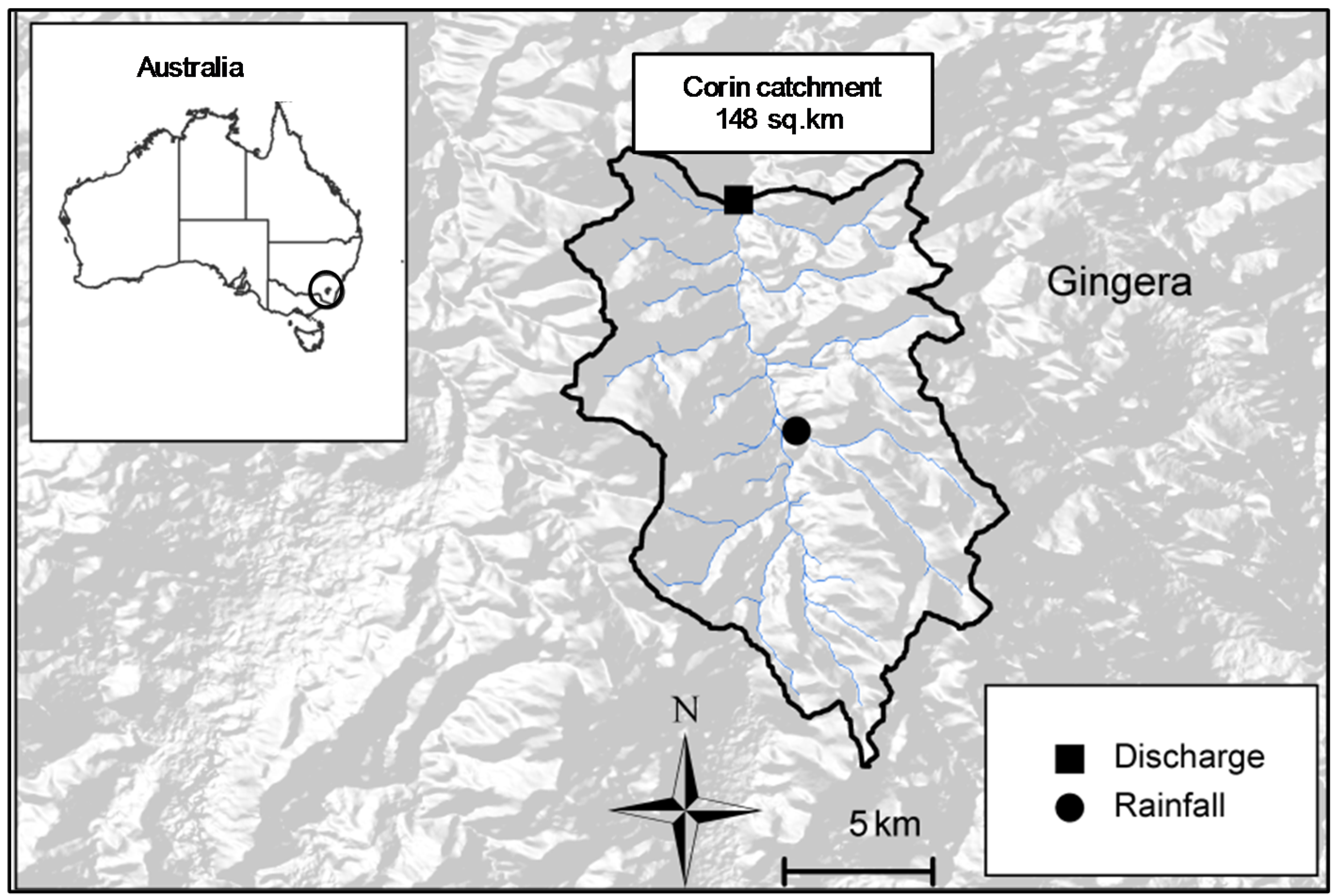
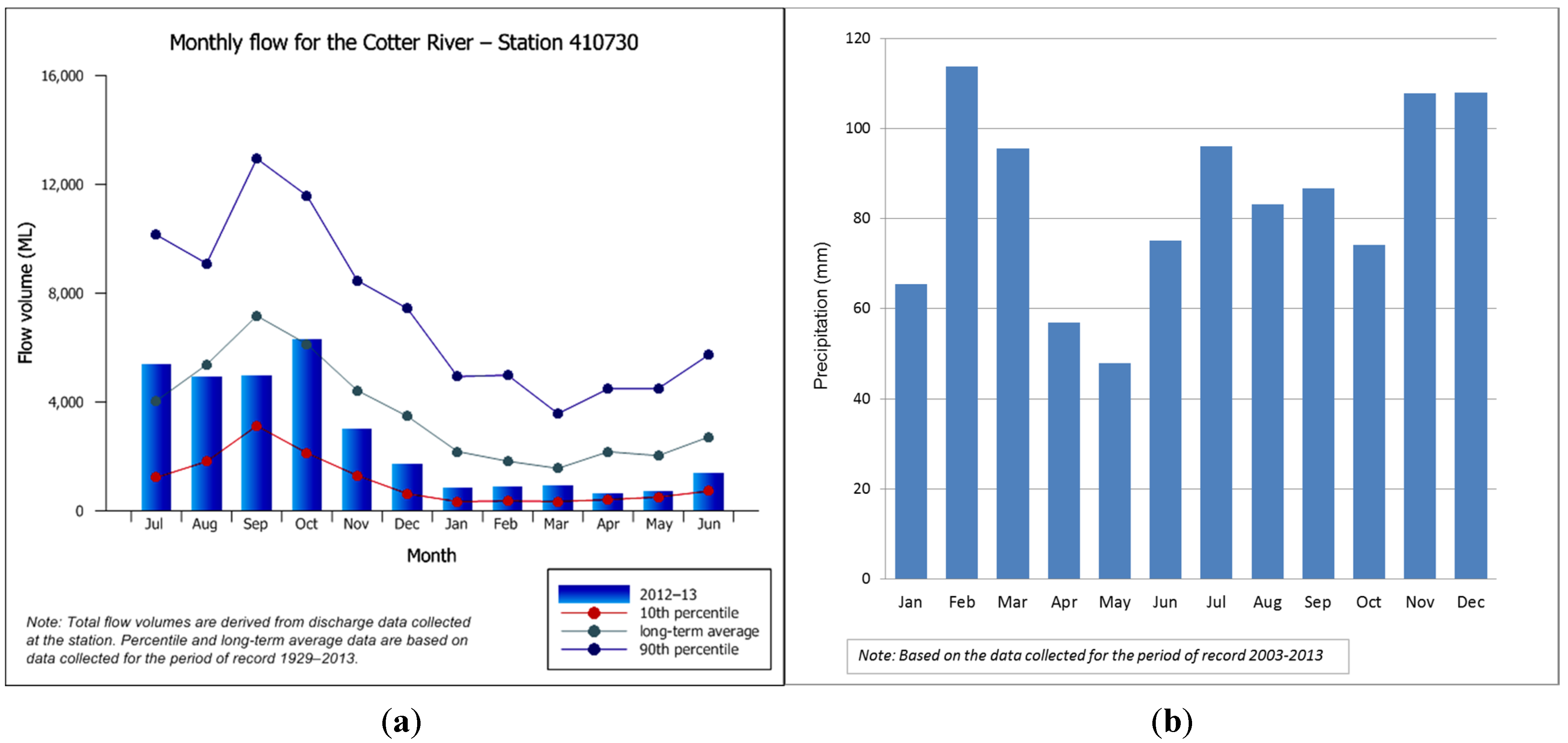
2.1. Case Study and Data Sources


2.2. Standardization and Goodness of Fit Criteria
- Root Mean Square Error (RMSE)
- Volume Error (VE)
- Correlation (Corr)
- Nash-Sutcliffe Efficiency (NSE)
2.3. Data-Driven Methods
- Non-Linear Multivariate Regression (NLMR)
- K-Nearest Neighbor (K-NN)
- (1)
- setting a matrix with m columns (number of predictors) and n + 1 rows (length of time series).
- (2)
- last row of the above-mentioned matrix is assumed as a vector of predictors at current time (xj,t j = 1:m).
- (3)
- remaining rows are assumed as a matrix of predictors at historical time series (xj,t-i j = 1:m i = 1:n).
- (4)
- vector Q is defined with n rows of independent variable values from t − n to t − 1.
- (5)
- using a distance function, distances between xj,t and xj,(t-i) are calculated.where wj are weights of predictor variables at the distance function. We chose the Euclidean function as the distance function with equal weights to predictor variables.
- (6)
- distance vector (Dist) is sorted from minimum to maximum (SDist) and vector Q is assorted based on SDist.
- (7)
- best number of neighbors (k) are specified based on a variety of methods. Here we have used the empirical equation in which n is the length of the time series which is used as historical data for calibration and validation stages [41].
- (8)
- (9)
- forecast value at current time is calculated as:where T is the transpose operation.
- Nonlinear Autoregressive with External Input Based Artificial Neural Networks (NARX-ANN)
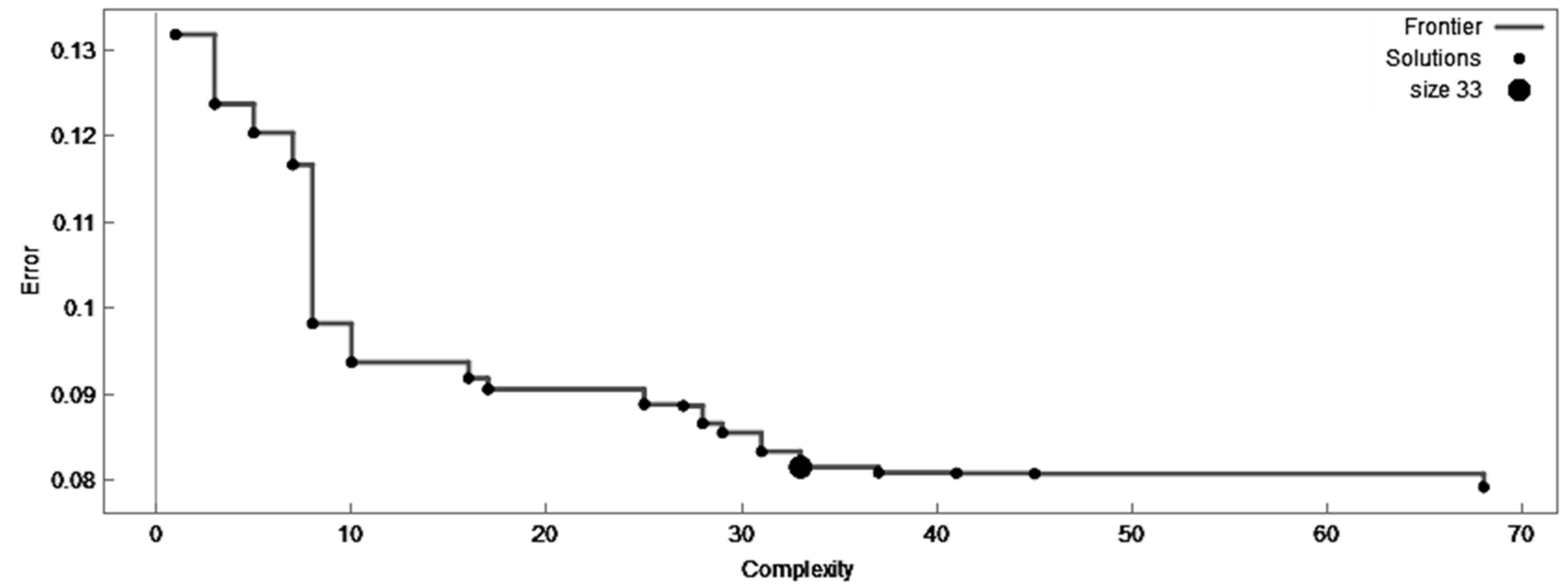
- Symbolic Regression (SR)
3. Results and Discussion


| Variable | Sensitivity | % Positive | Positive Magnitude | % Negative | Negative Magnitude |
|---|---|---|---|---|---|
| NDVIi-1 | 1.31 | 31% | 3.81 | 69% | 0.21 |
| WYi-1 | 0.70 | 55% | 1.16 | 45% | 0.14 |
| Precii-1 | 0.08 | 99% | 0.08 | 0% | 0 |
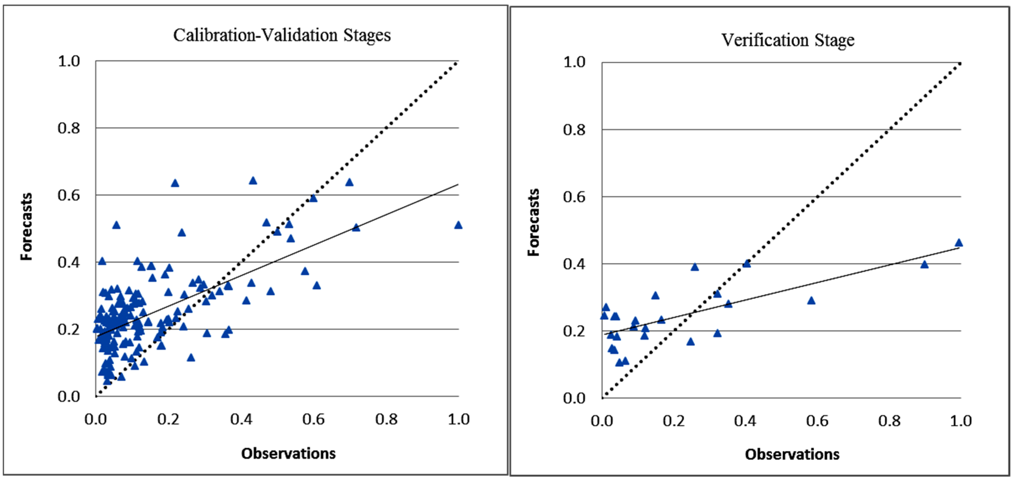
| Methods | Calibration-Validation (85% of Data) | Verification (15% of Data) | Entire Data | |||||||||
|---|---|---|---|---|---|---|---|---|---|---|---|---|
| Corr | RMSE | VE % | NSE | Corr | RMSE | VE % | NSE | Corr | RMSE | VE % | NSE | |
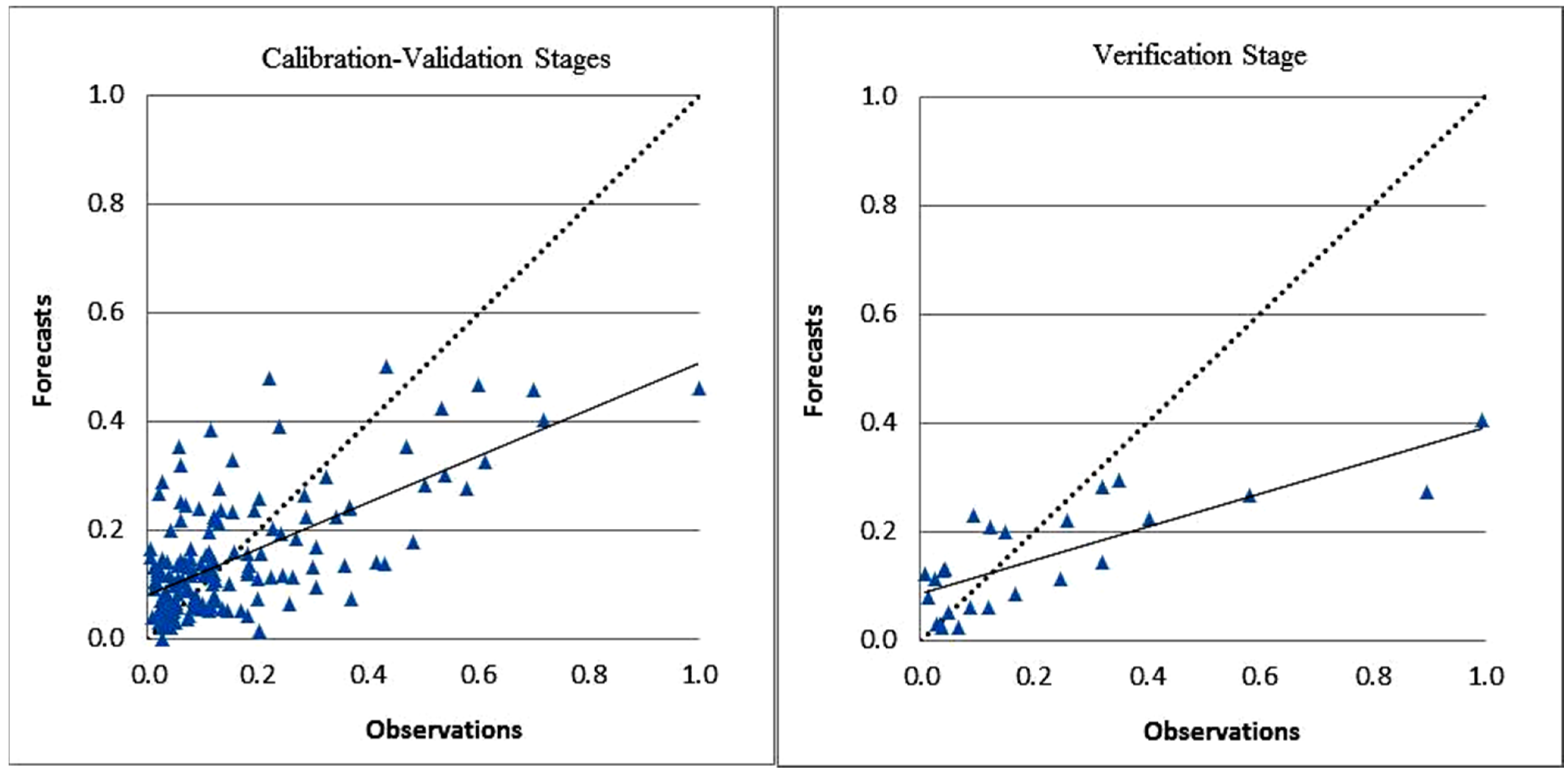
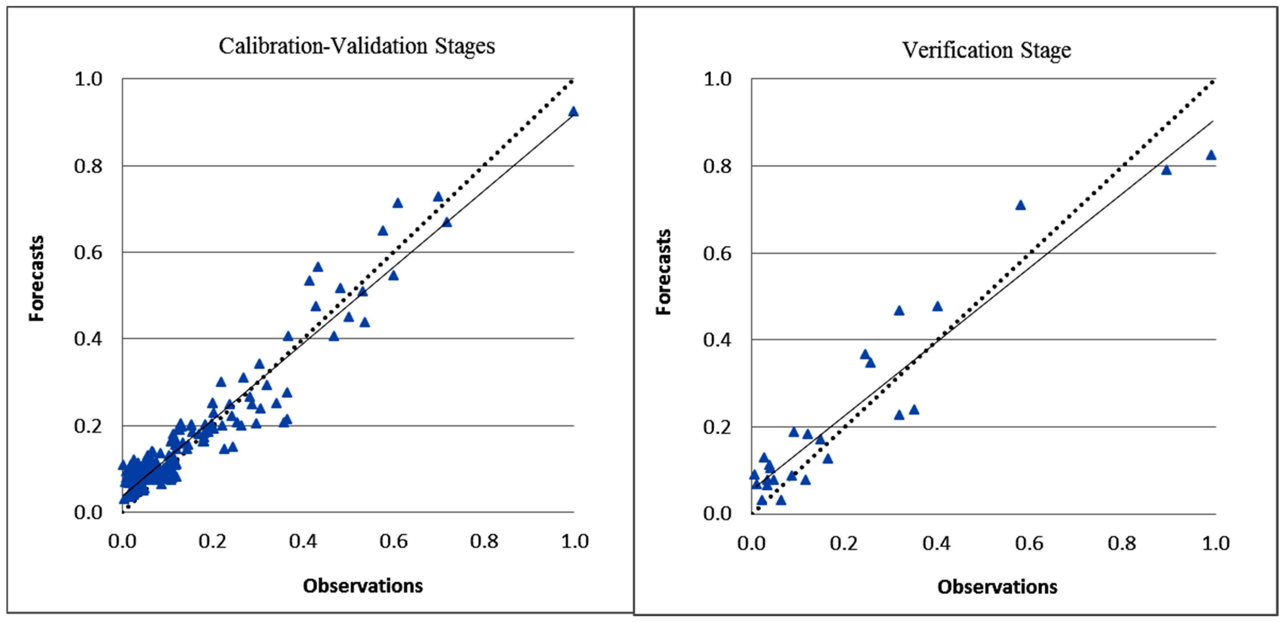
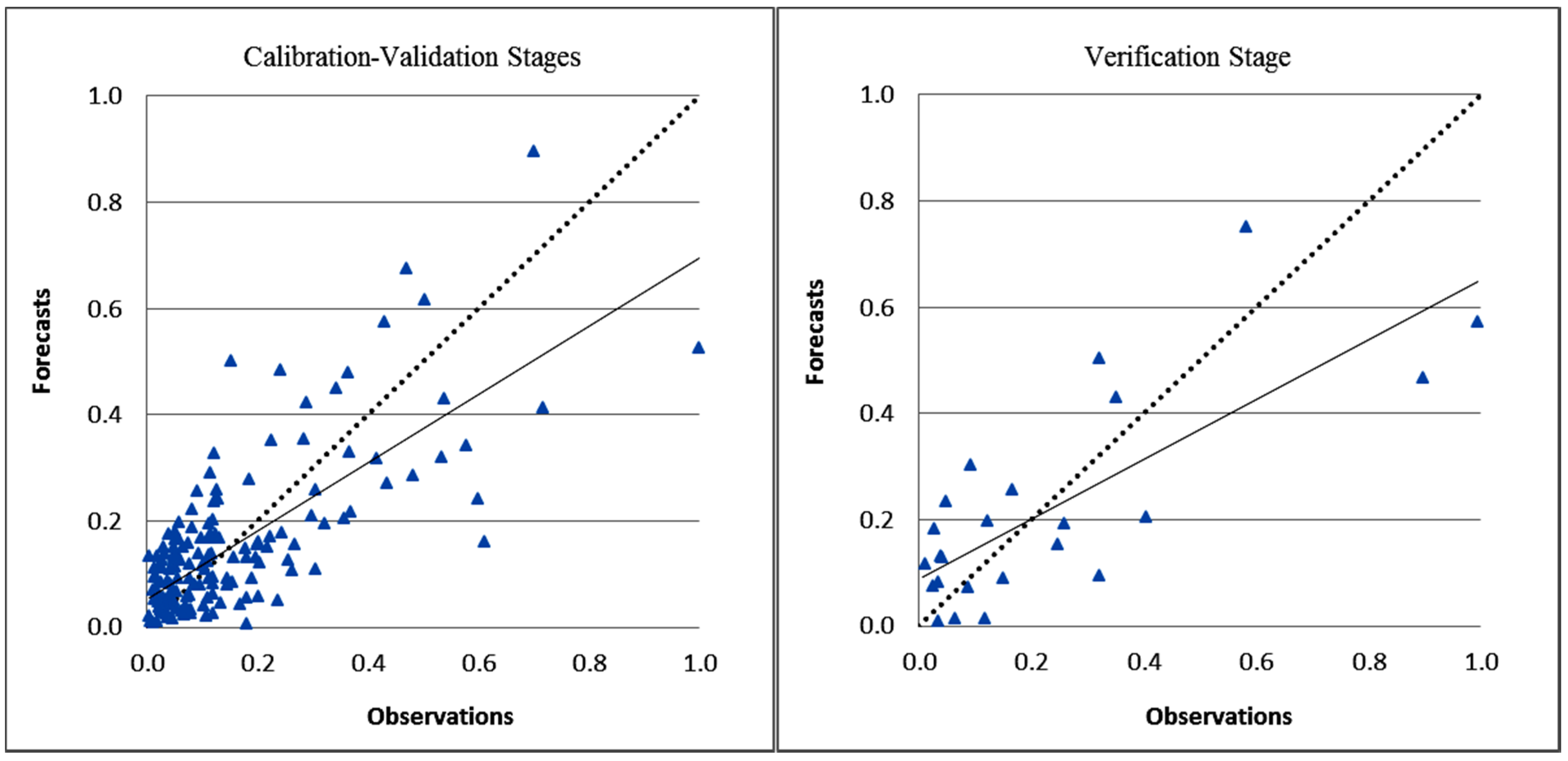
| K-NN | 0.64 | 0.16 | 3.42 | −0.10 | 0.74 | 0.21 | 3.57 | −3.54 | 0.63 | 0.17 | 3.44 | −0.33 |
| NLMR | 0.79 | 0.10 | 1.51 | 0.60 | 0.78 | 0.20 | 1.50 | 0.40 | 0.76 | 0.12 | 1.51 | 0.55 |
| NARX-ANN | 0.91 | 0.07 | 1.20 | 0.80 | 0.90 | 0.11 | 1.50 | 0.80 | 0.90 | 0.08 | 1.24 | 0.80 |
| SR | 0.82 | 0.09 | 1.09 | 0.67 | 0.80 | 0.16 | 1.20 | 0.63 | 0.82 | 0.10 | 1.16 | 0.67 |


4. Conclusions
Acknowledgments
Author Contributions
Conflicts of Interest
References
- Langford, K.J. Changes in yielf of water following a bushfire in a forest of Eucalyptus regnans. J. Hydrol. 1976, 29, 87–114. [Google Scholar] [CrossRef]
- Viggers, J.I.; Weaver, H.J.; Lindenmayer, D.B. Melbourne’s Water Catchments: Perspectives on a World-Class Water Supply; CSIRO Publishing: Collingwood, Australia, 2013. [Google Scholar]
- Kuczera, G. Prediction of water yield reductions following a bushfire in ash-mixed species eucalypt forest. J. Hydrol. 1987, 94, 215–236. [Google Scholar] [CrossRef]
- McMichael, C.E.; Hope, A.S. Predicting streamflow response to fire-induced landcover change: Implications of parameter uncertainty in the MIKE SHE model. J. Environ. Manag. 2007, 84, 245–256. [Google Scholar] [CrossRef]
- Marcar, N.E.; Benyon, R.G.; Polglase, P.J.; Paul, K.I.; Theiveyanathan, S.; Zhang, L. Predicting Hydrological Impacts of Bushfire and Climate Change in Forested Catchments of the River Murray Uplands: A Review; CSIRO, Water for a Healthy Country National Research Flagship: Canberra, Australia, 2006. [Google Scholar]
- Watson, F.G.R.; Vertessy, R.A.; Grayson, R.B. Large-scale modelling of forest hydrological processes and their long-term effect on water yield. Hydrol. Process. 1999, 13, 689–700. [Google Scholar] [CrossRef]
- Green, E.P.; Mumby, P.J.; Edwards, A.J.; Clark, C.D.; Ellis, A.C. Estimating leaf area index of mangroves from satellite data. Aquat. Bot. 1997, 58, 11–19. [Google Scholar] [CrossRef]
- Vertessy, R.A.; Watson, F.G.R.; O’Sullivan, S.K.; Davis, S.; Campbell, R.; Benyon, R.; Haydon, S.R. Predicting Water Yield from Mountain Ash Forest Catchments; Report 98/4; Cooperative Research Centre for Catchment Hydrology: Clayton, Australia, 1998. [Google Scholar]
- Turner, D.P.; Cohen, W.B.; Kennedy, R.E.; Fassnacht, K.S.; Briggs, J.M. Relationships between leaf area index and Landsat TM spectral vegetation indices across three temperate zone sites. Remote Sens. Environ. 1999, 70, 52–68. [Google Scholar] [CrossRef]
- Vertessy, R.A.; Watson, F.G.R.; O’Sullivan, S.K. Factors determining relations between stand age and catchment water balance in mountain ash forests. For. Ecol. Manag. 2001, 143, 13–26. [Google Scholar] [CrossRef]
- Abbott, M.B.; Bathurst, J.C.; Cunge, J.A.; O’Connell, E.; Rasmussen, J. An introduction to the European System: Systeme Hydrologique Europeen (SHE). J. Hydrol. 1986, 87, 61–77. [Google Scholar] [CrossRef]
- Muluye, G.Y.; Coulibaly, P. Seasonal reservoir inflow forecasting with low frequency climatic indices: A comparison of data-driven methods. Hydrol. Sci. J. 2007, 52, 508–522. [Google Scholar] [CrossRef]
- Londhe, S.; Charhate, S. Comparison of data-driven modelling techniques for river flow forecasting. Hydrol. Sci. J. 2010, 55, 1163–1174. [Google Scholar] [CrossRef]
- Noh, S.J.; Tachikawa, Y.; Shiba, M.; Kim, S. Ensemble kalman filtering and particle filtering in a lag-time window for short-term streamflow forecasting with a distributed hydrologic model. J. Hydrol. Eng. 2013, 18, 1684–1696. [Google Scholar] [CrossRef]
- Lee, H.; Mclntyre, N.R.; Wheater, H.S.; Young, A.R. Predicting runoff in ungauged UK catchments. Proc. ICE Water Manag. 2006, 159, 129–138. [Google Scholar] [CrossRef]
- Asquith, W.H.; Herrmann, G.E.; Cleveland, T.G. Generalized additive regression models of discharge and mean velocity associated with direct-runoff conditions in Texas: Utility of the U.S. geological survey discharge measurement database. J. Hydrol. Eng. 2013, 18, 1331–1348. [Google Scholar] [CrossRef]
- Asquith, W.H. Regression models of discharge and mean velocity associated with near-median streamflow conditions in Texas: Utility of the U.S. geological survey discharge measurement database. J. Hydrol. Eng. 2014, 19, 108–122. [Google Scholar] [CrossRef]
- Azmi, M.; Araghinejad, S.; Kholghi, M. Multi model data fusion for hydrological forecasting using K-nearest neighbour method. Iran. J. Sci. Technol. 2010, 34, 81–92. [Google Scholar]
- Akbari, M.; Overloop, P.J.V.; Afshar, A. Clustered K nearest neighbor algorithm for daily inflow forecasting. Water Resour. Manag. 2011, 25, 1341–1357. [Google Scholar] [CrossRef]
- Saghafian, B.; Anvari, S.; Morid, S. Effect of Southern Oscillation Index and spatially distributed climate data on improving the accuracy of Artificial Neural Network, Adaptive Neuro-Fuzzy Inference System and K-Nearest Neighbour streamflow forecasting models. Expert Syst. 2013, 30. [Google Scholar] [CrossRef]
- Nourani, V.; Komasi, M.; Alami, M.T. Hybrid wavelet-genetic programming approach to optimize ANN modeling of rainfall-runoff process. J. Hydrol. Eng. 2012, 17, 724–741. [Google Scholar] [CrossRef]
- Danandeh Mehr, A.; Kahya, E.; Olyaie, E. Streamflow prediction using linear genetic programming in comparison with a neuro-wavelet technique. J. Hydrol. 2013, 505, 240–249. [Google Scholar] [CrossRef]
- Yilmaz, A.G.; Muttil, N. Runoff estimation by machine learning methods and application to the euphrates basin in Turkey. J. Hydrol. Eng. 2014, 19, 1015–1025. [Google Scholar] [CrossRef]
- Araghinejad, S.; Azmi, M.; Kholghi, M. Application of artificial neural network ensembles in probabilistic hydrological forecasting. J. Hydrol. 2011, 407, 94–104. [Google Scholar]
- Singh, A.; Imtiyaz, M.; Issac, R.K.; Denis, D.M. Comparison of artificial neural network models for sediment yield prediction at single gauging station of watershed in eastern India. J. Hydrol. Eng. 2013, 18, 115–120. [Google Scholar] [CrossRef]
- Budu, K. Comparison of wavelet-based ANN and regression models for reservoir inflow forecasting. J. Hydrol. Eng. 2014, 19, 1385–1400. [Google Scholar] [CrossRef]
- Manel, S.; Dias, J.M.; Ormerod, S.J. Comparing discriminant analysis, neural networks and logistic regression for predicting species distributions: A case study with a Himalayan river bird. Ecol. Model. 1999, 120, 337–347. [Google Scholar] [CrossRef]
- Paruelo, J.; Tomasel, F. Prediction of functional characteristics of ecosystems: A copmarison of artificial neural networks and regression models. Ecol. Model. 1997, 98, 173–186. [Google Scholar] [CrossRef]
- Shamshiry, E.; Bin Mokhtar, M.; Abdulai, A. Comparison of Artificial Neural Network (ANN) and Multiple Regression Analysis for Predicting the Amount of Solid Waste Generation in a Tourist and Tropical Area—Langkawi Island; International Biological, Civil and Environmental Engineering: Dubai, United Arab Emirates, 2014. [Google Scholar]
- Talsma, T. Soils of the Cotter catchment area, ACT: Distribution, chemical and physical properties. Aust. J. Soil Res. 1983, 21, 241–255. [Google Scholar] [CrossRef]
- White, I.; Wade, A.; Daniell, T.M.; Mueller, N.; Worthy, M.; Wasson, R. The vulnerability of water supply catchments to bushfires: Impacts of the January 2003 wildfires on the Australian Capital Territory. Aust. J. Water Resour. 2006, 10, 179–194. [Google Scholar]
- Sparks, T.; Muller, N.; O’Shannassy, K.; Taylor, P. Cotter Catchment Landscape Analysis; ACTEW Corporation: Canberra, Australia, 2008. [Google Scholar]
- Xavier, A.C.; Vettorazzi, C.A. Monitoring leaf area index at watershed level through NDVI from Landsat-7/ETM+ data. Sci. Agric. 2004, 61, 243–252. [Google Scholar] [CrossRef]
- Huete, A.; Justice, C.; van Leeuwen, W. MODIS Vegetation Index (MOD 13) Algorithm Theoretical Basis Document ATBD13; The University of Arizona: Tucson, AZ, USA, 1999. [Google Scholar]
- Sever, L.; Leach, J.; Bren, L. Remote sensing of post-fire vegetation recovery; A study using Landsat 5 TM imagery and NDVI in North-East Victoria. J. Spat. Sci. 2012, 57, 175–191. [Google Scholar] [CrossRef]
- Coops, N.; Delahaye, A.; Pook, E. Estimation of eucalypt forest leaf area index on the south coast of New South Wales using Landsat MSS data. Aust. J. Bot. 1997, 45, 757–769. [Google Scholar] [CrossRef]
- Solano, R.; Didan, K.; Jacobson, A.; Huete, A. MODIS Vegetation Index User’s Guide; MOD13 Series; Collection 5; Vegetation Index and Phenology Lab, The University of Arizona: Tucson, AZ, USA, 2010. [Google Scholar]
- Hill, M.J.; Senarath, U.; Lee, A.; Zeppel, M.; Nightingale, J.M.; Williams, R.D.J.; McVicar, T.R. Assessment of the MODIS LAI product for Australian ecosystems. Remote Sens. Environ. 2006, 101, 495–518. [Google Scholar] [CrossRef]
- Nash, J.E.; Sutcliffe, J.V. River flow forecasting through conceptual models part I: A discussion of principles. J. Hydrol. 1970, 10, 282–290. [Google Scholar] [CrossRef]
- Schrage, L. Optimization Modelling with LINGO, 5th ed.; LINDO System Inc.: Chicago, IL, USA, 1999. [Google Scholar]
- Tarboton, D.G.; Sharma, A.; Lall, U. The use of non-parametric probability distribution in streamflow modeling. In Proceedings of the Sixth South African National Hydrological Symposium, University of Natal, Pietermaritzburg, South Africa, 4–6 September 1993; pp. 315–327.
- Yakowitz, S.J. Nonparametric density estimation, prediction, and regression for Markov sequences. J. Am. Stat. Assoc. 1985, 80, 215–221. [Google Scholar] [CrossRef]
- Yan, L.; Elgamal, A.; Cottrell, G.W. Substructure vibration NARX neural network approach for statistical damage inference. J. Eng. Mech. 2013, 139, 737–747. [Google Scholar] [CrossRef]
- AlHamaydeh, M.; Choudhary, I.; Assaleh, K. Virtual testing of buckling-restrained braces via nonlinear autoregressive exogenous neural networks. J. Comput. Civil Eng. 2013, 27, 755–768. [Google Scholar] [CrossRef]
- Ruslan, F.A.; Samad, A.M.; Zain, Z.M.; Adnan, R. Flood prediction using NARX neural network and EKF prediction technique: A comparative study. In Proceedings of the IEEE 3rd International Conference on System Engineering and Technology, Shah Alam, Malaysia, 19–20 August 2013.
- Koza, J.R.; Keane, M.A.; Streeter, M.J. Evolving Inventions; Scientific American: New York, NY, USA, 2003; pp. 40–47. [Google Scholar]
- Schmidt, M.; Lipson, H. Distilling free-form natural laws from experimental data. Science 2009, 324, 81–85. [Google Scholar] [CrossRef] [PubMed]
- Abrahart, R.J.; Beriro, D.J. How much complexity is warranted in a rainfall-runoff model? Findings obtained from symbolic regression, using Eureqa. In Proceedings of EGU General Assembly, Vienna, Austria, 22–27 April 2012.
- Grelle, G.; Bonito, L.; Revellino, P.; Guerriero, L.; Guadagno, F.M. A hybrid model for mapping simplified seismic response via a GIS-metamodel approach. Nat. Hazards Earth Syst. Sci. 2014, 2, 963–997. [Google Scholar] [CrossRef]
- Larsen, P.E.; Cseke, L.J.; Miller, R.M.; Collart, F.R. Modeling forest ecosystem responses to elevated carbon dioxide and ozone using artificial neural networks. J. Theor. Biol. 2014, 359, 61–71. [Google Scholar] [CrossRef] [PubMed]
- Drobot, R.; Dinu, C.; Draghia, A.; Adler, M.J.; Corbus, C.; Matreata, M. Simplified approach for flood estimation and propagation. In Proceedings of the IEEE International Conference on Automation, Quality and Testing, Robotics, Cluj-Napoca, Romania, 22–24 May 2014.
- Hamdan, M.A.; Bardan, A.A.; Abdelhafez, E.A.; Hamdan, A.M. Comparison of neural network models in the estimation of the performance of solar collectors. J. Infrastruct. Syst. 2014. [Google Scholar] [CrossRef]
- Coulibaly, P.; Bobee, B.; Antcil, F. Improving extreme hydrologic eventsforecasting using a new criterion for artificial neural network selection. Hydrol. Process. 2001, 15, 1533–1536. [Google Scholar] [CrossRef]
- Charhate, S.B.; Dandawate, Y.H.; Londhe, S.N. Genetic programming to forecast stream flow. Adv. Water Resour. Hydraul. Eng. 2009, 1–6, 29–34. [Google Scholar]
- McMillan, H.; Krueger, T.; Freer, J. Benchmarking observational uncertainties for hydrology: Rainfall, river discharge and water quality. Hydrol. Process. 2012, 26, 4078–4111. [Google Scholar] [CrossRef]
© 2015 by the authors; licensee MDPI, Basel, Switzerland. This article is an open access article distributed under the terms and conditions of the Creative Commons Attribution license (http://creativecommons.org/licenses/by/4.0/).
Share and Cite
Gharun, M.; Azmi, M.; Adams, M.A. Short-Term Forecasting of Water Yield from Forested Catchments after Bushfire: A Case Study from Southeast Australia. Water 2015, 7, 599-614. https://doi.org/10.3390/w7020599
Gharun M, Azmi M, Adams MA. Short-Term Forecasting of Water Yield from Forested Catchments after Bushfire: A Case Study from Southeast Australia. Water. 2015; 7(2):599-614. https://doi.org/10.3390/w7020599
Chicago/Turabian StyleGharun, Mana, Mohammad Azmi, and Mark A. Adams. 2015. "Short-Term Forecasting of Water Yield from Forested Catchments after Bushfire: A Case Study from Southeast Australia" Water 7, no. 2: 599-614. https://doi.org/10.3390/w7020599