Article

The Stability of Revegetated Ecosystems in Sandy Areas: An Assessment and Prediction Index

1
Shapotou Desert Research and Experimental Station, Cold and Arid Regions Environmental and Engineering Research Institute, Chinese Academy of Sciences, Lanzhou 730000, China
2
Key Laboratory of Stress Physiology and Ecology in Cold and Arid Regions Gansu Province, Lanzhou 730000, China
*
Author to whom correspondence should be addressed.
Water 2015, 7(5), 1969-1990; https://doi.org/10.3390/w7051969
Submission received: 28 December 2014 / Revised: 15 April 2015 / Accepted: 15 April 2015 / Published: 30 April 2015
(This article belongs to the Special Issue Hydro-Ecological Modeling)

Abstract

:
The stability and sustainability of revegetated ecosystems is a central topic in ecological research. In this study, long-term monitoring and focused research on vegetation, soil and soil moisture from 2006 to 2012 were used to develop a model for evaluating indices of ecosystem stability using the analytical hierarchy process method. The results demonstrated that rainfall (R), vegetation coverage (C), and surface soil moisture (S) were the three most influential factors among the 14 indicators considered in a revegetated desert area in the Tengger Desert, China. A stability index (SI) was defined as SI = VAR (R) × VAR (C)/VAR (S), and a comparative study was conducted to examine the stability index of the natural vegetation community. The SI was divided into three regimes: SI < 0.006 was stable, 0.006 ≤ SI < 0.015 was semi-stable, and 0.015 ≤ SI was unstable. The stable, semi-stable and unstable periods of revegetated ecosystems in our simulations were 191, 17 and 11 years, respectively, within the total modeling period of 219 years. These results indicated that the revegetated desert ecosystem would be stable in most years during the vegetation succession, and this study presents new ideas for future artificial vegetation management in arid desert regions.

Graphical Abstract

1. Introduction

Stability has frequently been considered an important characteristic of ecological systems because of its theoretical and practical significance [1,2,3,4]. However, the concept of ecosystem stability is complex and has often been discussed in vague terms because of the complex physical and biological structures or integrated functions [5]. This complexity also occurs in artificial ecosystems [6]. Grimm and Wissel (1997) [7] presented a review and analyzed ecological stability, addressing 163 definitions of 70 different ecological stability concepts. Constancy, resilience, persistence, resistance, elasticity, mathematical stability and other concepts have been discussed in the literature in relation to specific problems in various ecosystems [8,9]. In these studies, debates on complexity-stability and diversity-stability have provided points of contention [1,10]. Early studies suggested that simple ecosystems were less stable than complex ecosystems, but later studies came to the opposite conclusion [11]. Until recently, questions on the relationship between stability and complexity have not been answered [12,13,14]. However, for the diversity-stability debate, evidence from multiple ecosystems at a variety of temporal and spatial scales suggests that biological diversity acts to stabilize ecosystem functioning when presented with environmental fluctuations [1]. Moreover, variation among species in their response to such fluctuations is an essential requirement for ecosystem stability [15,16]. Thus, we can conclude that stability is a multi-dimensional concept that has scale-dependent features. Generally, ecosystem stability refers to the capacity of a natural system to apply self-regulating mechanisms and return to a steady state after an outside disturbance.
Ecologists have developed a variety of approaches to measure ecosystem stability [2,17,18,19]. In most cases, mathematical models or empirical methods are involved, with the former developed and expanded by Robert May in 1973 [20] using linear stability analysis on models constructed from a statistical universe (randomly constructed communities with randomly assigned interaction strengths). However, mathematically derived models are only suitable for characterizing the dynamic behavior of simple dynamic systems, whereas ecological systems are not usually uniform [21]. Most ecosystems operate in a variable environment that includes events at a wide range of frequencies and intensities, and it is often difficult to determine the degree of changes or disturbances. Empirical methods involve the development of a stability index that incorporates the main characteristics of ecosystem structure or environmental factors; the stability of an ecosystem can then be determined from these indicators [22,23]. However, this solution must still manage the problem of parameter selection [24]. For instance, in a forest ecosystem, stability may be described with biomass, diversity, dominant species density, nutrient cycling and soil characteristics, etc. Thus, developing a method that can combine quantitative measurements and qualitative descriptions is particularly pertinent when evaluating analyses of ecosystem stability. The best method for evaluating problems that involve a number of uncertain indices is the analytic hierarchy process (AHP) method [25,26,27]. The AHP is a multiple-criteria decision-making tool that has been widely applied in diverse fields, such as resource allocation, project design, maintenance management and policy evaluation. This method is particularly useful because it enables the decomposition of a given problem into a hierarchy of more easily comprehended sub-problems that can each be analyzed independently. The elements of the hierarchy can be related to any aspect of the qualitative and quantitative problems, including aspects that are tangible or intangible and carefully measured or roughly estimated. Once the hierarchy is built, the AHP systematically evaluates its various elements and derives numerical priorities for each of the decision alternatives [28,29]. Thus, one may easily apply the AHP to select promising technologies, and it provides a simple method for making decisions or performing environmental impact assessments [30,31,32]. However, relatively few studies have assessed the application of AHP to ecosystem stability [27,33,34], especially in revegetated desert areas.
Sand-binding vegetation has been widely used in arid desert regions and is considered one of the most effective methods of mitigating desertification [35]. However, in recent years, climate change and harsh natural environments have produced a series of problems, such as declining vegetation cover, poor plant growth and widespread water stress, which have led us to investigate the stability of artificial vegetation [6]. In this research, we hypothesized that the natural vegetation community is stable because natural vegetation in the study area is the result of long-term (i.e., over thousands of years) evolution [36]. Therefore, this hypothesis is reasonable, and several studies have also illustrated that ecosystems with artificial vegetation would become stable over plant succession, with these stabilizing changes mainly reflected in the increased vegetation cover and soil texture improvements compared with that of the adjacent natural vegetation communities [37,38,39]. However, these improvements are only concomitant with the individual process of vegetation succession, and a comprehensive system for evaluating stability indices, including the integration of vegetation, soil and water factors, is still lacking. Furthermore, previous studies primarily focused on qualitative concept models, and a quantitative model is not available. In the present study, over 50 years of vegetation succession and long-term monitoring data (2006–2012) from the Shapotou Desert Research and Experimental Station on the southeastern edge of the Tengger Desert were used to investigate soil and vegetation characteristics at different stages of plant succession. The key influencing factors of the ecosystem stability were then determined with the AHP method, and a stability index was defined. Finally, the ecosystem’s stability was predicted with a dynamical model of vegetation cover and soil moisture. Our results provide basic suggestions for sustainable ecosystem management and new hypotheses regarding vegetation succession models.

2. Materials and Methods
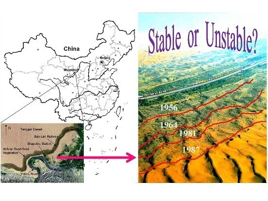
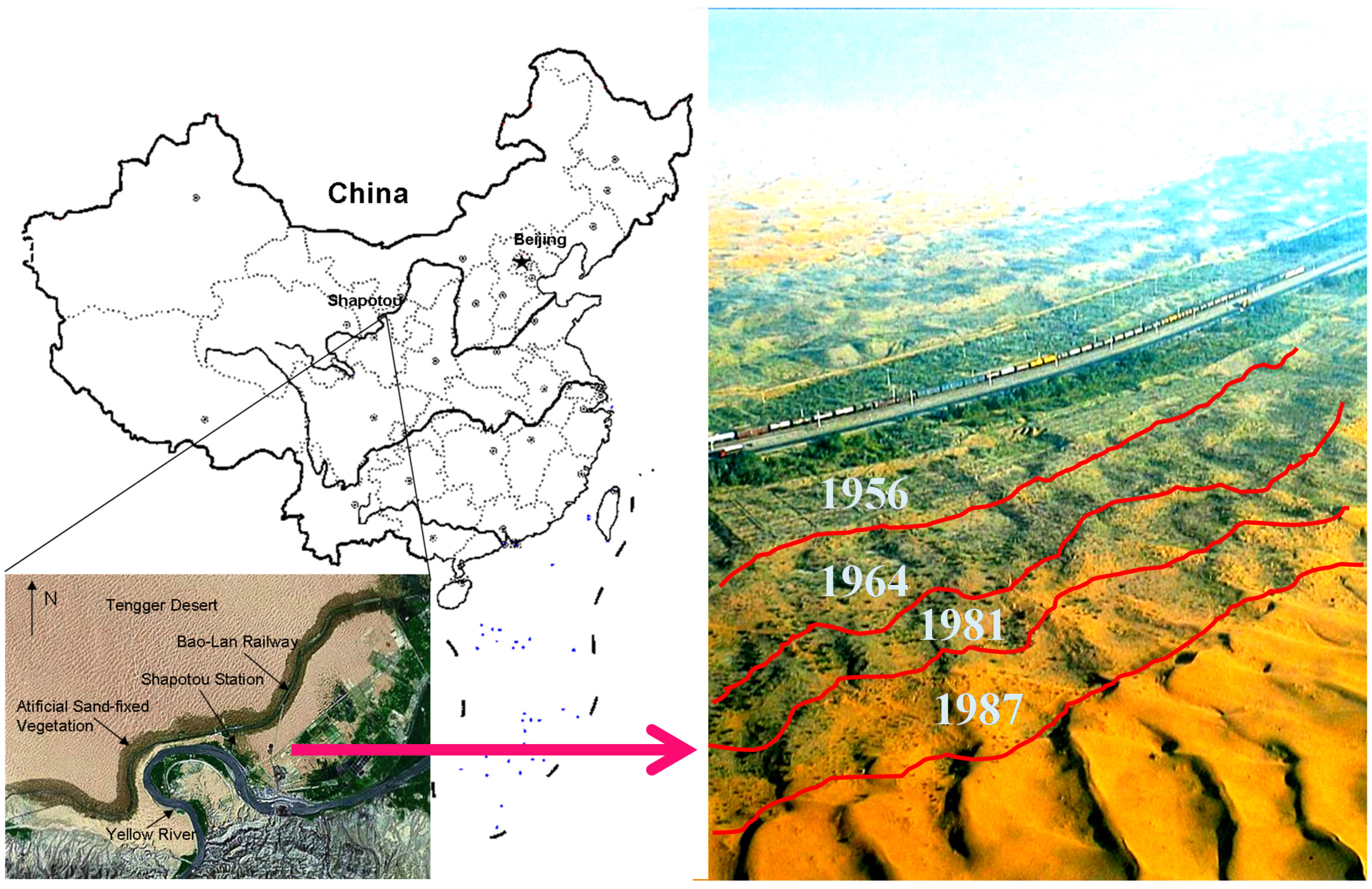
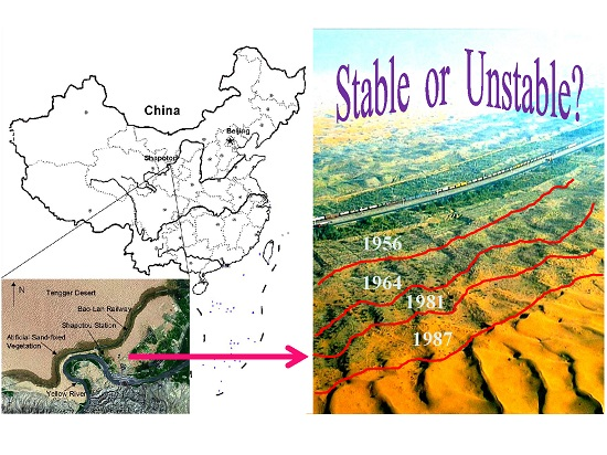
2.1. Study Site

The study was conducted at Shapotou Desert Research and Experimental Station of the Chinese Academy of Sciences, located in the Shapotou region at the southeastern margin of the Tengger Desert (37°32' N, 105°02' E). The climate at the site is characterized by abundant sunshine and low relative humidity. The average minimum monthly relative humidity is 33% in April, and the average maximum monthly relative humidity is 54.9% in August. The elevation of the area is 1330 m, and the mean annual precipitation is 188.2 mm according to meteorological records from 1956 to 2009, with rainfall occurring primarily between June and September [37]. The mean annual temperature is 9.6 °C, and the mean monthly temperatures are −6.9 °C in January and 24.3 °C in July. The evapotranspiration potential during the growing season (May to September) is 2300 to 2500 mm.
To ensure the smooth operation of the desert section of the Baotou-Lanzhou railway, a system involving sand-binding vegetation was established by the Chinese Academy of Sciences and other related departments in 1956. First, mechanical sand fences were installed at right angles to the prevailing winds, and then 1 m × 1 m straw sand barriers were erected in a checkerboard pattern behind the mechanical sand fences. Under non-irrigated conditions, xerophytic shrubs dominated by Caragana korshinskii, Artemisia ordosica, Hedysarum scoparium, Caragana intermedia, Calligonum arborescens and Atraphaxis bracteata were planted at a spacing of 1 m × 2 m or 2 m × 3 m using the checkerboard of straw barriers as a protective screen. This ecological shelter was extended in 1964, 1981 and 1987. As shown in Figure 1, a 16 km long protective system of vegetation was eventually established, and our research site was part of this protective system, which was 500 m wide on the north side and 200 m wide on the south side of the railway. Over the 50 years since the establishment of the vegetation, the environment in the area has improved, and the stabilized sand surface has created conditions that support the colonization of a number of species. The mass propagation of psammophytes has transformed the original moving sand into a complex man-made and natural desert vegetation landscape [37]. This ecological engineering project was viewed as a successful model for desertification control and ecological restoration along the transport line in the arid desert region of China. Because sites with different ages were stabilized using similar approaches, including the planting of shrub seedlings of the same species with the same density in similar straw checkerboards (see Table 1), they can represent the different successional stages of sand-binding vegetation.
Figure 1. Schematic description of the study site (revegetated in 1956a, 1964a, 1981a and 1987a) in the Shapotou region of the Tengger Desert, northwestern China.
Water 07 01969 g001
Table 1. Description of four revegetation sites with different ages and a natural community located in the southeastern fringe of the Tengger Desert, Northern China.
Year of RevegetationApproaches to Sand Stabilization and RevegetationRemaining Shrub Species of RevegetationNative/Invasion Dominant Plant Species
1956Straw-checkerboard of 1 m2 planted with 10 xerophytic shrubs at a density of 16 individuals per 100 m2Artemisia ordosica,
Caragana korshinskii,
Hedysarum scoparium
Artemisia ordosica,
Scorzonera mongolica,
Sonchus arvensis,
Chloris virgata,
Aristida adscensionis,
Setaria viridis,
Bassia dasyphylla,
Chenopodium aristatum
1964Straw-checkerboard of 1 m2 planted with 10 xerophytic shrubs at a density of 16 individuals per 100 m2Artemisia ordosica,
Caragana korshinskii,
Hedysarum scoparium
Artemisia ordosica,
Bassia dasyphylla,
Eragrostis poaeoides,
Sonchus arvensis,
Scorzonera mongolica,
Euphorbia humifusa
1981Straw-checkerboard of 1 m2 planted with 10 xerophytic shrubs at a density of 16 individuals per 100 m2Artemisia ordosica,
Caragana korshinskii,
C. microphylla,
Hedysarum scoparium
Artemisia ordosica,
Hedysarum scoparium,
Bassia dasyphylla,
Eragrostis poaeoides,
Corispermum patelliforme
1987Straw-checkerboard of 1 m2 planted with 10 xerophytic shrubs at a density of 16 individuals per 100 m2Amorpha fruticosa,
Artemisia ordosica,
A. sphaerocephala,
Caragana korshinskii,
C. microphylla,
Calligonum arborescens,
Hedysarum scoparium
Hedysarum scoparium,
Agriophyllum squarrosum,
Bassia dasyphylla,
Echinos gmelinii,
Eragrostis poaeoides
NaturalNoNoArtemisia ordosica,
Caragana korshinskii,
Lespedeza davurica,
Ceratoides latens,
Oxytropis aciphylla,
Stipa breviflora,
Carex stenophylloides,
Cleistogenes sogorica,
Allium mongolicum,
Oxytropis myriophylla,
Enneapogon brachystachyus,
Asparagus gobicus

2.2. Methods

2.2.1. Sampling Method and Data Collection

Three 10 m × 10 m quadrats were established in each of the fixed observation plots in the sand-binding vegetation districts established in previous years (1956, 1964, 1981 and 1987) as well as in the adjacent natural vegetation zones for a total of 15 quadrats. The plant species number, height, and coverage for each species in the sand stabilization areas of different years were recorded or measured monthly from 2006 to 2012. Plant diversity (H′) was estimated with the Shannon–Wiener index for each region and month according to the formula: H′ =∑pilnpi, where p is the proportion of each species i. Precipitation was recorded every 30 min using tipping bucket-type rain gauges (Casella) and Campbell CR30X data-loggers (Campbell Scientific, Logan, UT, USA). Samples were collected monthly with a soil auger, and the soil moisture of the samples was determined using the oven-drying method (0–40 cm) and neutron moisture probe method (40–300 cm). To avoid confusion between the surface and deep soil moisture, the gravimetric moisture content of the surface soil layer and bulk density measurements were used to calculate the volumetric moisture content.
Soil parameters were measured at depths of 0–20 cm at each site during the growing season in 2006 and 2010. In each plot, 100 soil sampling points were mechanically arranged in 10 m × 10 m vegetation plots of different ages. The transverse and longitudinal spacing were both 1 m. The surface of the sampling plots was flat, and composite samples were sieved through a 2 mm mesh screen and used for further analysis. Particle size was analyzed using the pipette method [40], and soil bulk density was measured using the ring-cutting method [41]. Soil organic carbon (SOC) was determined according to the dichromate oxidation method of Walkley–Black [42]. Total nitrogen was measured with a Kjeltec System 1026 Distilling Unit (Tecator AB, Hoganas, Sweden), and electrical conductivity (EC) was determined by preparing a suspension that consisted of a soil–water mixture in a ratio of 1:5 and was measured using a portable conductivity meter (Cole-Parmer Instrument Company, Vernon Hills, IL, USA). Topographic parameters (elevation, slope angle and aspect) were determined with a Real-Time Kinematic (RTK) global positioning system (GPS) (S86T, Southern Technology, Guangzhou, China) in 2006.
In this study, we chose the commonly applied method of space-for-time substitution, which assumes that simultaneous sampling of different sites of different ages is equivalent to resampling the same site through time [36]. The clay percentage was selected to represent the soil texture, and soil organic matter and total N content were used to reflect the soil nutrient regime. According to the depth distribution of the mass root systems of herbaceous plants and shrubs, the soil moisture content at 0–40 cm and 40–300 cm, respectively, were determined. The clay percentage was measured because soil texture is considered an important factor that determines the vegetation structure and composition under uniform climatic conditions, whereas soil moisture was measured because it is considered a driving force for ecological processes in arid zones. Thus, these indices can reflect the overall stability of the ecosystem [38].

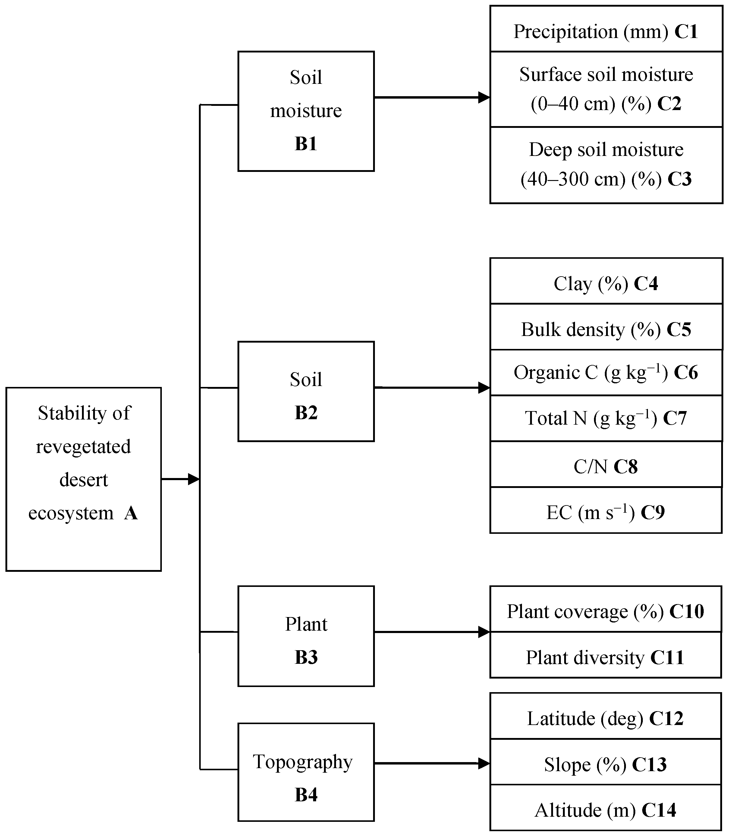
2.2.2. Analytic Hierarchy Process Methodology

The AHP method was applied to select the major influencing factors from the above datasets. The AHP procedure involves three basic steps: (i) Design of the decision hierarchy; (ii) Pair-wise comparison of elements of the hierarchical structure; and (iii) Construction of an overall priority rating. For more details, refer to Appendix A.1. In this study, fourteen important criteria were selected to evaluate the stability of the revegetated desert ecosystem (Figure 2). The top level of the diagram shows the overall goal of the hierarchy, “stability of revegetated desert ecosystems”; the second level lists the most influential factors obtained from other literature [36,37], such as soil moisture, soil characteristics, plant cover and topography; and the third level describes the attributes of each factor. After defining the criteria for selecting the evaluating index, five comparison matrices were developed: A–B, B1–C, B2–C, B3–C and B4–C. At each level, the criteria were compared pairwise according to their levels of influence and according to the specified criteria at the higher level. In AHP, multiple pairwise comparisons are based on a standardized comparison scale of nine levels, and ten experts were asked to perform pair-wise comparisons using a 1–9 preference scale that indicates the importance or dominance of one element over another. On this preference scale, 1 indicates equal preference and 9 indicates absolute preference. Intermediate values are used to express increasing preference/performance for one weight/alternative [43]. For example, if the criteria for soil moisture (B1) were judged as essential or of moderate importance, then the soil criteria (B2) with respect to the preservation of revegetated desert ecosystem stability would be given a score of 3. In addition, for other pairwise comparisons matrices, such as B2–C, the degree of importance was determined by the number of years of recovery required to reach the level of native ecosystem, such as desert steppe [36]. All of the important factors were then assigned appropriate weights, and a standardization index was calculated with the Z-score method. Finally, the integrated index was calculated, and the most influential factors in the revegetated ecosystem were determined.
Figure 2. A hierarchy for the stability evaluation of revegetated desert ecosystems.
Water 07 01969 g002

2.2.3. Coupled Dynamics of Soil Moisture and Vegetation

Soil water is the major driving force shaping vegetation patterns and processes in desert areas; however, plant growth, vegetation succession or landscape variability may also generate temporal and spatial heterogeneity of soil moisture [6]. Thus, to predict dynamic changes in soil water and vegetation succession in arid desert regions, a simplified ecohydrological box model that contains the coupled dynamics of vegetation and soil moisture was selected [44]. The model is as follows:
d s d t = I ( s , t ) [ b x b ( s ) + ( 1 b ) x 0 ( s ) ]
d b d t = g ( s ) b ( 1 b ) u ( s )
In Equation (1), s is the relative soil moisture averaged over the root zone (0 ≤ s ≤ 1) and b is the fraction of vegetated sites, where 0 < b < 1. Variations in site occupancy depend on the rate at which empty sites are colonized and the rate at which vegetated sites become vacant as a result of mortality. I(s, t) is the infiltration rate (mm day−1); Xb and X0 denote evapotranspiration (mm day−1), which is distinct between vegetated and bare sites; g(s) denotes the colonization rate; and u(s) denotes the local extinction rate (year1). All of the aforementioned rates were dependent on soil moisture. Each item in Equation (1) and the above parameter values are detailed in Appendix A.2. Matlab 7.0 (The MathWorks, Natick, MA, USA) and Origin 7.0 (OriginLab, Northampton, MA, USA) software were used for data simulation and analysis.

3. Results

3.1. Results of the Analytic Hierarchy Process (AHP) Application

Following the input of each factor and its importance into the expert choice and quantitative approach functions, the comparison results and weights of the four main criteria were calculated, and they are shown in Table 2. The results (principal vectors) show that the attributes have the following approximate priority weights: Soil moisture (0.91), soil (0.22), plant cover (0.23), and topography (0.28). The consistency ratio (CR) for this comparison was 0.086 < 0.10, which indicated that the weighted results were valid and consistent. In contrast, if the CR value were larger than the acceptable value of 0.10, the matrix results would be inconsistent and exempt from further analysis. Similarly, pair-wise comparisons of the sub-criteria indices with respect to the four criteria in the middle level were conducted. The comparison and weight results for this level are shown in Table 3, Table 4, Table 5 and Table 6. The final stage of the AHP was to compute the contribution of each index to the overall goal, and the global weights were calculated by multiplying the local weights with criteria and sub-criteria. The final weights and ranking of the indices were then obtained as shown in Table 7. The ranking of critical ecosystem stability factors showed that soil moisture and plant factors are the most influential. The highest-ranked factor was precipitation (0.86), followed by plant coverage (0.25) and surface soil moisture (0.23). The CR values of all matrices were less than 0.10 and were therefore accepted. The largest value in the priority weight was the most important criterion, which means that precipitation, surface soil moisture and plant coverage were the three most influential factors determining the stability of the revegetated desert ecosystem.
Table 2. Judgment matrix of the objective hierarchy and the criterion hierarchy.
AB1B2B3B4PrioritiesAHP Criteria
B11.003.005.004.000.91 λ m a x = 4.23;
CI = 0.078;
RI = 0.900;
CR = 0.086
B20.331.000.501.000.22
B30.202.001.000.500.23
B40.251.002.001.000.28
Notes: The weight of four evaluation criteria: Stability of revegetated desert ecosystem (A); Soil moisture (B1); Soil (B2); Plant (B3); Topography (B4).
Table 3. Judgment matrix of the criterion B1 and its related factors.
B1C1C2C3PrioritiesAHP Criteria
C11.005.004.000.95 λ m a x = 3.09; CI = 0.047;
RI = 0.58; CR = 0.081.
C20.201.002.000.26
C30.250.501.000.18
Notes: The weight of three evaluation criteria: Soil moisture (B1); Precipitation (C1); Surface soil moisture (0–40cm) (C2); Deep soil moisture (40-300cm) (C3).
Table 4. Judgment matrix of the criterion B2 and its related factors.
B2C4C5C6C7C8C9PrioritiesAHP Criteria
C41.000.332.001.005.000.500.27 λ m a x = 6.04;
CI = 0.008;
RI = 1.24;
CR = 0.006.
C53.001.005.003.009.002.000.78
C60.500.201.000.503.000.330.15
C71.000.332.001.005.000.500.27
C80.200.110.330.201.000.140.06
C92.000.503.002.007.001.000.47
Notes: The weight of nine evaluation criteria: Soil (B2); Clay (C4); Bulk density (C5); Organic C (C6); Total N (C7); C/N (C8); EC (C9).
Table 5. Judgment matrix of the criterion B3 and its related factors.
B3C10C11PrioritiesAHP Criteria
C101.005.000.98 λ m a x = 2; CI = 0;
RI = 0.00; CR = 0.
C110.201.000.20
Notes: The weight of two evaluation criteria: Plant (B3); Plant coverage (C10); Plant diversity (C11).
Table 6. Judgment matrix of the criterion B4 and its related factors.
B4C12C13C14PrioritiesAHP Criteria
C121.001.0020.63254 λ m a x = 3.02; CI = 0.008;
RI = 0.58; CR = 0.013.
C131.001.0030.72389
C140.50.3310.27546
Notes: The weight of three evaluation criteria: Topography (B4); Latitude (C12); Slope (C13); Altitude (C14).
Table 7. Overall weight of the ecosystem stability evaluation index.
IndicesB1B2B3B4Overall Priorities
0.910.220.230.28
C10.950.86
C20.260.23
C30.180.16
C40.270.06
C50.780.18
C60.150.03
C70.270.06
C80.060.01
C90.470.11
C100.980.25
C110.200.05
C120.630.18
C130.720.20
C140.280.08
CI = 0.052; RI = 0.955; CR = 0.055<0.1

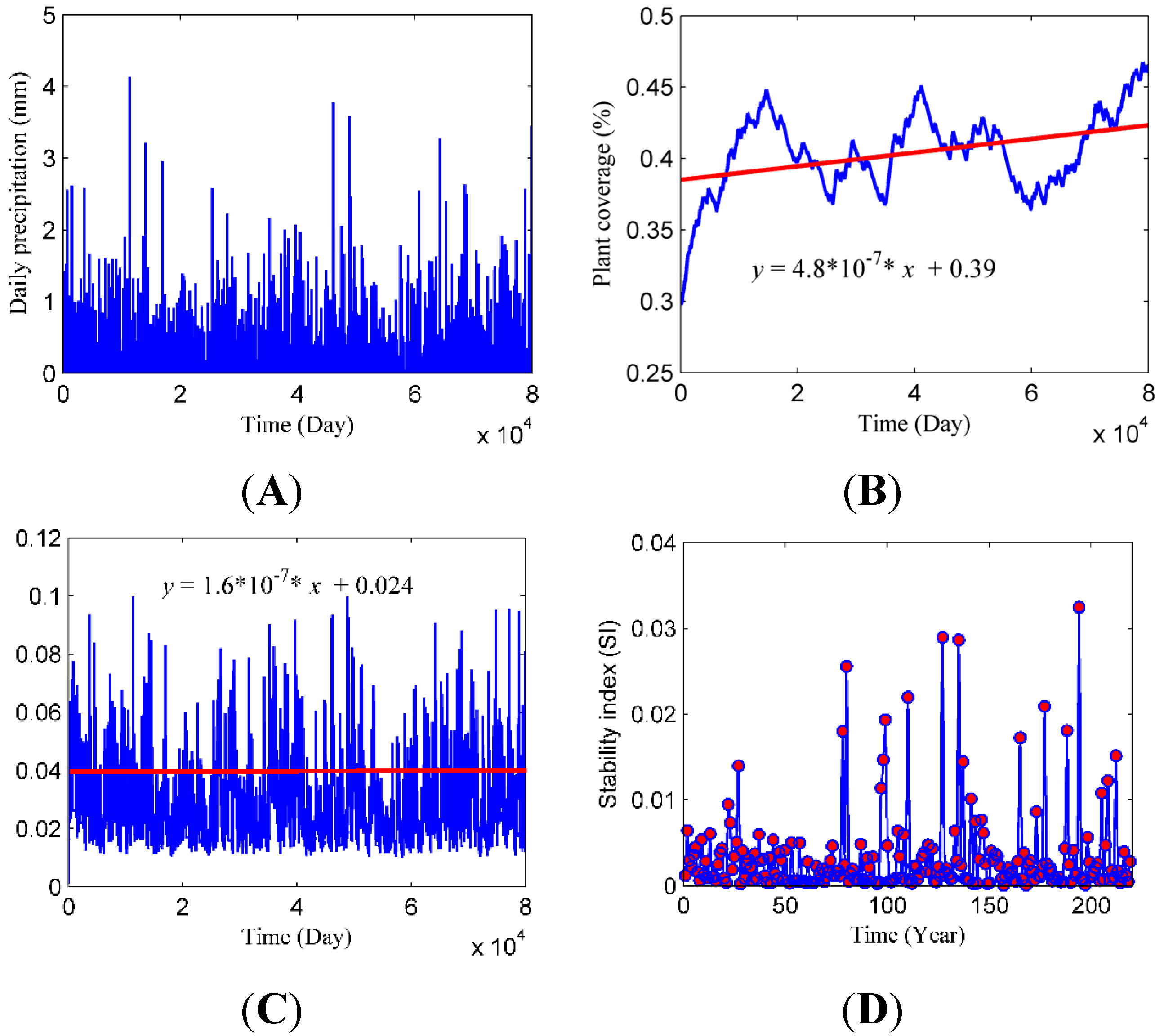
3.2. Stability Index Definition, Measurement and Prediction

The above AHP analysis verified that precipitation (C1), surface soil moisture (C2) and plant coverage (C10) were the three main limiting factors that affected the stability of the ecosystem; the stability index (SI) was therefore defined as SI = VAR (C1) × VAR (C10) / VAR (C2). VAR denotes the variance of a random variable. Generally, we assumed that the natural vegetation has higher stability; thus, the greater the similarity of different successional stages of sand-binding vegetation, the higher its stability. As shown in Figure 3A–D, plant coverage and surface soil moisture depended on annual precipitation. In particular, the maximum annual rainfall in 2007 was 271.2 mm, which induced extensive plant growth; in contrast, in 2006, 2009 and 2010, the annual rainfall was only approximately 100 mm, and plant coverage and surface soil moisture were maintained at a relatively low level. However, the amplitude of plant coverage was less than that of surface soil moisture in different vegetative sites. The SI in the natural vegetation site was 0.005, and it was 0.011, 0.012, 0.013, 0.017 in the 1956a, 1964a, 1981a and 1987a vegetation sites, respectively. The above results suggest that with increasing years of sand-binding vegetation, the revegetated desert ecosystem would become more stable. However, when compared with the natural vegetation, ecological restoration in arid desert regions still occurred over a very long time scale.
At long time scales, we have simulated 219 years of rainfall, vegetation coverage and soil moisture changes from Equation (1), as shown in Figure 4A–C. Numerical results have shown that soil moisture and vegetation cover would increase in the future and that the soil moisture would be maintained at 2.5%, but the rate of increase was not very high. The vegetation coverage remained at 40%, with fluctuations, but it was still increasing, and the rate of increase of vegetation coverage was larger than that of soil moisture. The SI also fluctuated with ecosystem succession, most of which was closer to the natural vegetation, as shown in Figure 3D. Based on the above-measured data and its distribution patterns, the SI can be divided into several regimes, which we defined as follows: SI < 0.006 was stable, 0.006 ≤ SI < 0.015 was semi-stable and 0.015 ≤ SI was unstable. Thus, the stable, semi-stable and unstable periods in our simulations were 191, 17 and 11 years within the total 219 years, respectively, which indicated that the revegetated desert ecosystem would be stable the majority of the time.
Figure 3. (A) Annual precipitation; (B) plant coverage; (C) soil moisture and (D) stability index of different vegetative sites and the control; The horizontal dashed lines represents the threshold of ecosystem stability, SIs = 0.004, SIus = 0.015.
Water 07 01969 g003
Figure 4. (A) Simulated results of daily precipitation; (B) plant coverage; (C) soil moisture and (D) stability index using Equation (1) over 219 years.
Water 07 01969 g004

4. Discussion

Stability is an important indicator of ecosystem health and a necessary condition for ecosystem sustainability [4]. The assessment of ecosystem stability is helpful in revealing community dynamics and vegetation succession [2]. Debate is ongoing regarding the definition of stability [1], and each researcher has individual evaluation methods, which is because of regional differences or specific research objectives [14]. Therefore, in the present study, ecosystem stability was measured with the comparative method, and natural vegetation ecosystems were considered stable. In these ecosystems, natural vegetation indicators, such as plant coverage or soil moisture, were assumed to represent the standard, and ecosystems that are closer to this standard are more stable. This approach avoids theoretical controversy and provides a simple method for practical applications. In revegetated desert ecosystems, soil moisture, soil characteristics, plant cover and topography were selected as the integral influential factors for ecosystem stability. For the selection of useful variables, the AHP method was used because it effectively incorporates interdependent criteria and local problems involving both quantitative and qualitative issues. A key drawback in using the AHP method is the requirement of pair-wise comparison that must be completed by experts because such expert judgments may be affected by factors, such as fatigue and impatience during this process, especially when a large number of criteria or alternatives are involved [45]. To avoid this drawback, a reasonable and manageable number of criteria were contained in the model. Another alternative is the Bayesian inference [46], which works very well if opinions among the experts are strongly divergent, and different prior parameters can be used to test for robustness [47,48]. In this study, based on results from the literature and information gleaned from discussions with ten experts, who are authorities on eco-hydrology in arid desert areas and were unified in their feedback, the AHP method was chosen in this study, and a total of fourteen criteria were determined. Using the AHP method, we verified that precipitation, surface soil moisture and plant coverage were the key limiting factors for artificial vegetation stability in arid desert regions. Precipitation was considered the sole source of water replenishment in this area, and soil water was the main driving force of the ecosystem’s patterns and processes. Additionally, the changes in the vegetation patterns also affected the redistribution of precipitation and infiltration depth in different soil layers. Therefore, these ecohydrological processes and their feedback mechanisms were identified as the main problems affecting the restoration and reconstruction of certain ecological engineering projects in arid regions [6]. However, for other ecosystems (such as agro-ecosystems, grasslands or forests), ecosystem structure and function are more complicated than in revegetated desert ecosystems [36,37,38]; therefore, evaluating ecosystem stability is more difficult [3,4,6]. Thus, a Bayesian methodology that provides for semiautomatic searches of consensus building should be considered instead of AHP.
To quantify the stability indicators, we defined the SI as the integration of variance of three variables. Because precipitation and surface soil moisture were inextricably linked, they always varied at the same time. Therefore, we defined the ratio of the two as a coefficient, and then multiplied it by the variance of vegetation cover, which directly represents the ecosystem restoration or degradation within a certain period. Thus, the stability of the ecosystem is specific, quantitative and verifiable. Simulated results from Equation (1) have shown that the ecosystem may become unstable in years with high precipitation because years with high annual precipitation are often followed by several years of continuous drought [49,50], which dramatically changes soil moisture and vegetation cover. This greater fluctuation leads to instability of the revegetated ecosystem. Compared with other empirical stability indices, such as community numbers, biomass or plant diversity [51], our stability index is simple and practical. Furthermore, it reflects the intrinsic characteristics of ecosystem stability, such as stochastic dynamics and temporal dependence, and accurately reflects the entire ecosystem with real environmental fluctuations. The SI values of different vegetation sites were then compared with the natural vegetation community, and stable or unstable regimes were determined. Based on field observations, the results showed that revegetated ecosystems increase in stability over time after the establishment of sand-binding vegetation. This conclusion is also supported by other studies in which the establishment of planted sand-binding vegetation in the Shapotou region is suggested to promote the improvement and restoration of regional habitats and provide suitable conditions for an increase in biodiversity in the desert ecosystem [37].
In terms of the mechanism by which sand-fixing vegetation promotes stability in the Tengger Desert, studies present inconsistent results on the formation mechanisms of stable plant communities. Shen (1986) [52] considered that A. ordosica may form a relatively stable climax community or plagioclimax, with the originally planted shrubs, such as C. korshinskii, H. scoparium and A. ordosica, degrading nearly 20 years later and withdrawing from the community. Zhao et al. (1988) [53] predicted that the next stage of vegetation succession would be herb-dominated plant communities. Li (2005) [38] advanced a conceptual model and stated that the revegetated plants would lead toward herb-dominated vegetation, which is similar to the primary vegetation types of the adjacent steppified desert and desert steppe. These results suggest that vegetation adapts to the habitat and revegetated ecosystems form a new equilibrium with vegetation succession. However, these previous studies were conceptual models, and vegetation succession assessments cannot be quantified. In the present study, a simplified dynamical model originally developed by Baudena et al. (2007) [44] that has been widely used in vegetation pattern analyses in arid and semi-arid areas [54,55] was applied, and it was capable of inferring the vegetation pattern features and useful information on underlying processes, including the susceptibility of the system to abrupt shifts to a desert state (i.e., unvegetated) as a result of climate change or anthropogenic disturbances [56]. Through our model simulations and the division of stability intervals, we predict that sand-fixing vegetation ecosystems will remain stable for a long period of time, although this stability will be interspersed with a number of semi-stable and unstable years. For certain theories or proposed mechanisms for the maintenance of ecosystem stability, such as the diversity theory or redundancy theory [57], self-organization of plant behaviors during a particular period of time is an essential component of vegetation succession over long time scales. Similar to banded or spot vegetation in North America, Africa and Australia [58,59,60], we could hypothesize that such self-organization reflects the normal vegetation successional pattern at different stages and suggest that vegetation may follow a “banded-spot-banded-spot (…)” pattern. Therefore, variations in vegetation composition, structure and responses to hydrological processes in the sand-binding areas are necessary stages of natural succession [61]. Thus, in artificial vegetation ecosystem management, the human should not be overly interfered with.

5. Conclusions

In this study, long-term monitoring and focused research was used to develop, measure and evaluate an index of ecosystem stability. Using the AHP method, we verified that rainfall (R), vegetation coverage (C) and surface soil moisture (S) are the three most influential factors in a revegetated desert area in the Tengger Desert, China. Over short time scales, the stability of the revegetated sandy ecosystem increased with years of succession. However, the stability of the artificial vegetation ecosystem may fluctuate with vegetation succession on a timescale of hundreds of years. The revegetated desert ecosystem was mostly stable based on our established theoretical system of ecosystem assessment and prediction, thus verifying the success of this method for desertification control and ecological restoration along a transport line in arid desert regions. Furthermore, our results provide new ideas for future artificial vegetation management and sustainable development in arid revegetated desert areas.

Acknowledgments

This work was supported by the National Key Basic Research program (2013CB429905) and Chinese National Natural Scientific Foundation (41201084; 41201086; 31170385).

Author Contributions

Conceived and designed the experiments: Lei Huang; Performed the experiments: Zhishan Zhang; Analyzed the data: Lei Huang; Contributed reagents/materials/analysis tools: Zhishan Zhang; Wrote the paper: Lei Huang. All authors read and approved the final manuscript.

Appendix

A.1. Analytic process hierarchy (AHP) methodology

AHP is a multi-criteria analysis method that is based on pair-wise comparisons of the components of a particular problem. This method enables a complex problem to be broken into a goal, criteria, solutions and other levels to provide a simple method for decision-making. Applying the AHP procedure involves three basic steps [62]: (1) Decomposition, or the hierarchy construction; (2) Comparative judgments, or defining and executing data collection to obtain pair-wise comparison data on elements of the hierarchical structure and (3) Synthesis of priorities, or constructing an overall priority rating.
In the first stage, a complex decision problem is structured as a hierarchy. This structure comprises a goal or focus at the topmost level, multiple criteria that define alternatives in the middle, and decision alternatives at the bottom. The second step is the comparison of the alternatives and the criteria. Once the problem has been decomposed and the hierarchy is constructed, prioritization procedure starts in order to determine the relative importance of the criteria within each level. The pairwise judgment starts from the second level and finishes in the lowest level. In each level, a nominal scale is used for the evaluation. The scale used in AHP for preparing the pairwise comparison matrix is a discrete scale from 1 (the two choice options are equally preferred) to 9 (one choice option is extremely preferred over the other), as presented in Table A1.
Table A1. Evaluation Scale in AHP.
Intensity of ImportanceDefinitionExplanation
1Equal ImportanceTwo elements have equal importance regarding the element in higher level
3Moderate ImportanceExperience or judgement slightly favours one element
5Strong ImportanceExperience or judgement strongly favours one element
7Very Strong ImportanceDominance of one element proved in practise
9Extreme ImportanceThe highest order dominance of one element over another
2,4,6,8Compromises between the AboveWhen compromise is needed
AdverseAdverse ComparisionsThe adverse evaluation of the same criteria, adverse of the same point under multiplication
Elements in each level are compared in pairs with respect to their importance to an element in the next higher level. Starting at the top of the hierarchy and working down, the pair wise comparisons at a given level can be reduced to a number of square matrices A = ( a i i ) n × n as in the following:
A = [ a 11 a 12 ... a 1 n a 21 a 22 ... a 2 n ... ... ... ... a n 1 a n 2 ... a n n ]   a i i = 1 ,   a j i = 1 / a i j ,   a i j 0
After all pair wise comparison matrices are formed, the vector of weights, w = ( w 1 , w 2 , ... , w n ) is computed on the basis of Sattys eigenvector procedure. The computation of the weights involves two steps. First, the pair wise comparison matrix A = ( a i i ) n × n is normalized by Equation (A1) and then the weights are computed by Equation (A2).
a i i * = a i j i = 1 n a i j ,  for all  j   = 1,2,..., n
w i = j = 1 n a i j * n ,  for all  j   = 1,2,..., n
Satty (1980) showed that there is a relationship between the vector weights, w and the pair wise comparison matrix, A, as shown in Equation (A3).
A w = λ max w
The λ max value is an important validating parameter in AHP and is used as a reference index to screen information by calculating the Consistency Ratio (CR) of the estimated vector. To calculate the CR, the Consistency Index (CI) for each matrix of order n can be obtained from Equation (A4).
C I = λ max n n 1
Then, CR can be calculated using Equation (A5):
C R = C I R I
Where RI is the random consistency index obtained from a randomly generated pair wise comparison matrix. Table A2 shows the value of the RI from matrices of order 1 to 10 as suggested by Satty [28]. If CR < 0.1, then the comparisons are acceptable. If, however, CR ≥ 0.1, then the values of the ratio are indicative of inconsistent judgments. In such cases, one should reconsider and revise the original values in the pair wise comparison matrix A.
Table A2. Random Indicators.
n12345678910
RI000.580.901.121.241.321.411.451.49

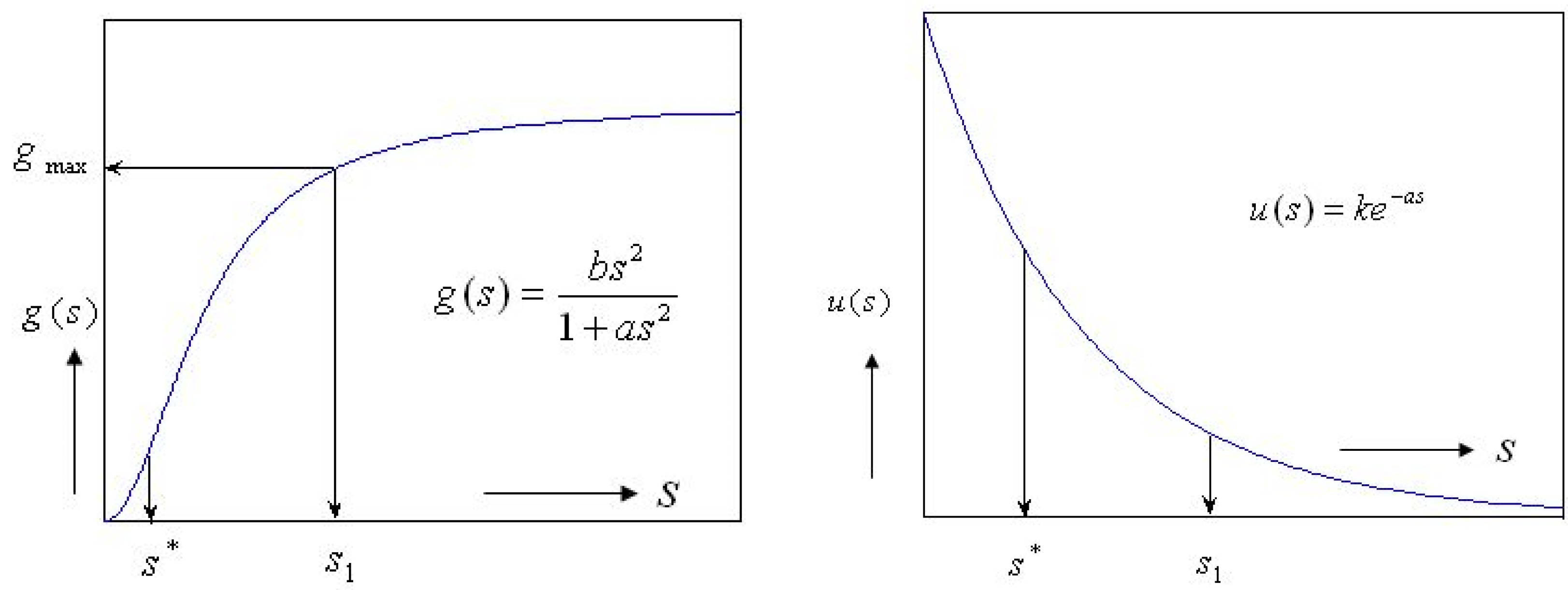
A.2. The Coupled Soil-Vegetation Model

The coupled soil-vegetation system (B1) was original presented in Baudena et al. (2007) [44], and we have improved some items in the equation as following, which would give a better description in our research area.
d s d t = I ( s , t ) [ b x b ( s ) + ( 1 b ) x 0 ( s ) ] d b d t = g ( s ) b ( 1 b ) u ( s ) b
where s is relative soil moisture averaged over the root zone ( 0 s 1 ), The fraction of vegetated sites is denoted by b ( 0 b 1 ). The infiltration rate I ( s , t ) is assumed to be equal to the rainfall rate, as long as the soil layer is not saturated; when rainfall exceeds the available water storage in the soil, the excess is converted into surface runoff. Thus,
I = { r n Z r r Δ t n Z r < 1 s 1 s Δ t r Δ t n Z r 1 s
where Δ t = 1 day. n is soil porosity and Z r is the active soil depth in millimeters. r is daily rainfall, which is modeled as instantaneous events occurring according to a marked Poisson process of rate (mean frequency of rainfall events) λ, and with exponentially distributed depths with mean h. x b ( s ) was the water losses from vegetated soil, which include direct soil evaporation and plant transpiration, s * is the critical soil moisture value below which plants start reducing transpiration by closing their stomata, and s 1 is the soil field capacity above which leakage occurs. The losses from evapotranspiration are assumed to increase linearly as a function of s until the moisture reaches a threshold s * , above which the evapotranspiration takes place at a maximum value E max , when the soil moisture exceeds the soil field capacity s 1 , the leakage losses was start by an exponential growth and reaching the saturated hydraulic conductivity k s at s =1.
x b ( s ) = { E max s * s E max E max + k s e β ( s s 1 ) 1 e β ( 1 s 1 ) 1   0 s < s * s * s < s 1 s 1 s < 1
x 0 ( s ) was the water losses in bare soil; E s o i l is pure soil evaporation before the leakage occurs. It increases linearly up to field capacity s 1 , above which the leakage losses was start with the same expression as for the vegetated soil.
x b ( s ) = { E s o i l s 1 s E s o i l + k s e β ( s s 1 ) 1 e β ( 1 s 1 ) 1   0 s < s 1 s 1 s < 1
the colonization and extinction rates g ( s ) and u ( s ) depend on s, as seen in the Figure A1, it can be modeled as:
g ( s ) = 0.05 s 2 1 + 12.36 s 2 ,   u ( s ) = 0.0006 e 4.69 s
Figure A1. Sketch for vegetation colonization rate and extinction rate.
Water 07 01969 g005
When the soil moisture was below the field capacity s 1 , plant growth was slowly at first and then reached to its maximum g max sharply with increased soil moisture, which have showed a typical “S” curve. The extinction rate is assumed to exponential decreased with soil moisture. The parameters for Matlab simulation were shown in Table A3.
Table A3. Parameters of the simplified ecohydrological box model.
ParametersSymbol (Unit)Value
Soil porosityn0.43
Active soil depthZr (cm)40
Critical soil moisture below which plant undergoes water stresss*0.11
Field capacitys10.56
Pore size distribution parameterβ12.7
Saturated hydraulic conductivityKs (cm/d)800
Pure soil evaporation E s o i l (mm/d) 0.1
Maximum evapotranspiration rate E max (mm/d)3.67
Average rainfall frequencyλ (/d)0.15
Average precipitation depthh (mm/d)0.61
The parameters in the model were obtained from the directly measured data. The cutting ring method was used to determine soil porosity n and field capacity s1 of root zone (3 repeats at the 0, 20 and 40 cm soil depths, respectively, and take the average). The saturated soil hydraulic conductivity Ks was measure by using of the tension infiltrometer model SW 080B (SDEC, Paris, France) in undisturbed field conditions; s* and another soil parameters β were determined according to related reference [63]. the historical precipitation information such as average rainfall frequency and depth were extracted from the receive data at a near weather station, and minor calibration was done by referring to the experiential relationship between precipitation and elevation. The depth of active soil or root zone depth, defined as the soil depth range in which 95% below-ground biomass were distributed, was determined by filed investigation. Pure soil evaporation Esoil were measured with micro-lysimeters, which were made using PVC pipes that were 30 cm high and 10 cm in internal diameter [64]. And maximum evapotranspiration rate Emax were determined with the combination of the stem heat balance technique (Dynamax Inc., Houston, TX, USA), the observations was measured continuous during the 2008-2012 growing season [65].

Conflicts of Interest

The authors declare no conflicts of interest.

References

  1. McCann, K.S. The diversity-stability debate. Nature 2000, 405, 228–233. [Google Scholar] [CrossRef] [PubMed]
  2. Tilman, D.; Reich, P.B.; Knops, J.M.H. Biodiversity and ecosystem stability in a decade long grassland experiment. Nature 2006, 441, 629–632. [Google Scholar] [CrossRef] [PubMed]
  3. Allesina, S.; Tang, S. Stability criteria for complex ecosystems. Nature 2012, 483, 205–208. [Google Scholar] [CrossRef] [PubMed]
  4. Donohue, I.; Petchey, O.L.; Montoya, J.M.; Jackson, A.L.; McNally, L.; Viana, M.; Healy, K.; Lurgi, M.; O’Connor, N.E.; Emmerson, M.C. On the dimensionality of ecological stability. Ecol. Lett. 2013, 16, 421–429. [Google Scholar] [CrossRef] [PubMed]
  5. Hill, A.R. Ecosystem stability, some recent perspectives. Prog. Phys. Geogr. 1987, 11, 315–333. [Google Scholar] [CrossRef]
  6. Li, X.R.; Zhang, Z.S.; Huang, L.; Wang, X.P. Review of the ecohydrological processes and feedback mechanisms controlling sand-binding vegetation systems in sandy desert regions of China. Chin. Sci. Bull. 2013, 58, 1483–1496. [Google Scholar] [CrossRef]
  7. Grimm, V.; Wissel, C. Babel, or the ecological stability discussions, an inventory and analysis of terminology and guide for avoiding confusion. Oecologia 1997, 109, 323–334. [Google Scholar] [CrossRef]
  8. Cottingham, K.L.; Brown, B.L.; Lennon, J.T. Biodiversity may regulate the temporal variability of ecological systems. Ecol. Lett. 2001, 4, 72–85. [Google Scholar] [CrossRef]
  9. Deimeke, E.; Cohena, M.J.; Reissb, K.C. Temporal stability of vegetation indicators of wetland condition. Ecol. Indic. 2013, 34, 69–75. [Google Scholar] [CrossRef]
  10. Ives, A.R.; Carpenter, S.R. Stability and diversity of ecosystems. Science 2007, 317, 58–62. [Google Scholar] [CrossRef] [PubMed]
  11. Pimm, S.L. The complexity and stability of ecosystems. Nature 1984, 307, 321–326. [Google Scholar] [CrossRef]
  12. Haydon, D.T. Pivotal assumptions determining the relationship between stability and complexity: An analytical synthesis of the stability complexity debate. Am. Nat. 1994, 144, 14–29. [Google Scholar] [CrossRef]
  13. Townsend, S.E.; Haydon, D.T.; Matthews, L. On the generality of stability complexity relationships in Lotka-Volterra ecosystems. J. Theor. Biol. 2010, 267, 243–251. [Google Scholar] [CrossRef] [PubMed]
  14. Mougi, A.; Kondoh, M. Diversity of interaction types and ecological community stability. Science 2012, 337, 349–351. [Google Scholar] [CrossRef] [PubMed]
  15. Cleland, E.E. Biodiversity and ecosystem stability. Nat. Education Knowl. 2012, 3, 14. [Google Scholar]
  16. Sterk, M.; Gort, G.; Klimkowska, A.; van Ruijven, J.; van Teeffelen, A.J.A.; Wamelink, G.W.W. Assess ecosystem resilience: Linking response and effect traits to environmental variability. Ecol. Indic. 2013, 30, 21–27. [Google Scholar] [CrossRef]
  17. Mitchell, R.J.; Auld, M.H.D.; Le Duc, M.G.; Marrs, R.H. Ecosystem stability and resilience, a review of their relevance for the conservation management of lowland heaths. Perspect. Plant Ecol. 2000, 3, 142–160. [Google Scholar] [CrossRef]
  18. Ives, A.R.; Dennis, B.; Cottingham, K.L.; Carpenter, S.R. Estimating community stability and ecological interactions from time series data. Ecol. Monogr. 2003, 73, 301–330. [Google Scholar] [CrossRef]
  19. Loreau, M.; de Mazancourt, C. Biodiversity and ecosystem stability, a synthesis of underlying mechanisms. Ecol. Lett. 2013, 16, 106–115. [Google Scholar] [CrossRef] [PubMed]
  20. May, R.M. Qualitative stability in model ecosystems. Ecology 1973, 54, 638–641. [Google Scholar] [CrossRef]
  21. Grimm, V.; Schmidt, E.; Wissel, C. On the application of stability concepts in ecology. Ecol. Model. 1992, 63, 143–161. [Google Scholar] [CrossRef]
  22. Wardle, D.A.; Bonner, K.I.; Barker, G.M. Stability of ecosystem properties in response to above-ground functional group richness and composition. Oikos 2000, 89, 11–23. [Google Scholar] [CrossRef]
  23. Hooper, D.U.; Chapin, F.S.I.; Ewel, J.J.; Hector, A.; Inchausti, P.; Lavorel, S.; Lawton, J.H.; Lodge, D.M.; Loreau, M.; Naeem, S.; et al. Effects of biodiversity on ecosystem functioning, a consensus of current knowledge. Ecol. Monogr. 2005, 75, 3–35. [Google Scholar] [CrossRef] [Green Version]
  24. Dale, V.H.; Beyeler, S.C. Challenges in the development and use of ecological indicators. Ecol. Indic. 2001, 1, 3–10. [Google Scholar] [CrossRef]
  25. Saaty, T.L. A scaling method for priorities in hierarchical structures. J. Math. Psychol. 1977, 15, 234–281. [Google Scholar] [CrossRef]
  26. Locantore, N.W.; Tran, L.T.; O’Neill, R.V.; McKinnis, P.W.; Smith, E.R.; O’Connell, M. An overview of data integration methods for regional assessment. Environ. Monit. Assess. 2004, 94, 249–261. [Google Scholar] [CrossRef] [PubMed]
  27. Zhang, R.Q.; Zhang, X.D.; Yang, J.Y.; Yuan, H. Wetland ecosystem stability evaluation by using analytical hierarchy process AHP, approach in Yinchuan Plain: China. Math. Comput. Model. 2013, 57, 366–374. [Google Scholar] [CrossRef]
  28. Saaty, T.L. The Analytical Hierarchy Process: Planning, Priority Setting, Resource Allocation; McGraw-Hill: New York, NY, USA, 1980. [Google Scholar]
  29. Vaidya, O.S.; Kumar, S. Analytic hierarchy process, An overview of applications. Eur. J. Oper. Res. 2006, 169, 1–29. [Google Scholar] [CrossRef]
  30. Banai, R. Anthropocentric problem solving in planning and design, with analytic hierarchy process. J. Archit. Plann. Res. 2005, 22, 107–120. [Google Scholar]
  31. Cheng, E.W.L.; Li, H.; Yu, L. The analytic network process (ANP), approach to location selection: A shopping mall illustration. Onstr. Innov. 2005, 5, 83–97. [Google Scholar] [CrossRef]
  32. Ho, W. Integrated analytic hierarchy process and its applications—A literature review. Eur. J. Oper. Res. 2008, 186, 211–228. [Google Scholar] [CrossRef]
  33. Barzekar, G.; Aziz, A.; Mariapan, M.; Ismail, M.H.; Hosseni, S.M. Using analytical hierarchy Pprocess (AHP), for prioritizing and ranking of ecological indicators for monitoring sustainability of ecotourism in northern forest: Iran. Ecologia Balkanica 2011, 3, 59–67. [Google Scholar]
  34. Convertino, M.; Baker, K.M.; Vogel, J.T.; Lu, C.; Suedel, B.; Linkov, I. Multi-criteria decision analysis to select metrics for design and monitoring of sustainable ecosystem restorations. Ecol. Indic. 2013, 26, 76–86. [Google Scholar] [CrossRef]
  35. Le Houerou, H.N. Restoration and rehabilitation of arid and semiarid Mediterranean ecosystems in North Africa and West Asia, a review. Arid Soil Res. Rehabil. 2000, 14, 3–14. [Google Scholar] [CrossRef]
  36. Li, X.R.; He, M.Z.; Duan, Z.H.; Xiao, H.L.; Jia, X.H. Recovery of topsoil physiochemical properties in revegetated sites in the sand-burial ecosystems of the Tengger Desert: Northern China. Geomorph 2007, 88, 254–265. [Google Scholar] [CrossRef]
  37. Li, X.R.; Xiao, H.L.; Zhang, J.G.; Wang, X.P. Long-term ecosystem effects of sand-binding vegetation in the Tengger Desert: Northern China. Restor. Ecol. 2004, 12, 376–390. [Google Scholar] [CrossRef]
  38. Li, X.R. Influence of variation of soil spatial heterogeneity on vegetation restoration. Sci. China Ser. D 2005, 35, 361–370. [Google Scholar] [CrossRef]
  39. Eldridge, D.J.; Koen, T.B.; Harrison, L. Plant composition of three woodland communities of variable condition in the western Riverina, New South Wales, Australia. Cunninghamia 2007, 10, 189–198. [Google Scholar]
  40. Loveland, P.J.; Walley, W.R. Particle size analysis. In Soil and Environmental Analysis, Physical Methods, 2nd ed.; Simth, K.A., Mullins, C.E., Eds.; Marcel Dekker: New York, NY, USA, 2001. [Google Scholar]
  41. Nanjing Institute of Soil Research. Analysis of Soil Physic-Chemical Features; Shanghai Science and Technology Press: Shanghai, China, 1980. [Google Scholar]
  42. Nelson, D.W.; Sommers, L.E. Total Carbon, Organic Carbon and Organic Matter. In Methods of Soil Analysis Part 2: Chemical and Microbiological Properties, 2nd ed.; Page, A.L., Miller, R.H., Keeney, D.R., Eds.; American Society of Agronomy, Soil Science Society of America: Madison, WI, USA, 1982; pp. 539–577. [Google Scholar]
  43. Cinelli, M.; Coles, S.R.; Kirwan, K. Analysis of the potentials of multi criteria decision analysis methods to conduct sustainability assessment. Ecol. Indic. 2014, 46, 138–148. [Google Scholar] [CrossRef]
  44. Baudena, M.; Boni, G.; Ferraris, L.; von Hardenberg, J.; Provenzale, A. Vegetation response to rainfall intermittency in drylands, results from a simple ecohydrological box model. Adv. Water Res. 2007, 30, 1320–1328. [Google Scholar] [CrossRef]
  45. Lee, J.K.L.; Chan, E.H.W. The analytic hierarchy process AHP, approach for assessment of Urban renewal proposals. Soc. Indicat. Res. 2008, 89, 155–168. [Google Scholar] [CrossRef]
  46. Altuzarra, A.; Moreno-Jiménez, J.M.; Salvador, M. Consensus building in AHP-group decision making: A Bayesian approach. Oper. Res. 2010, 58, 1755–1773. [Google Scholar] [CrossRef]
  47. Cagno, E.; Caron, F.; Mancini, M.; Ruggeri, F. Using AHP in determining the prior distributions on gas pipeline failures in a robust Bayesian approach. Reliab. Eng. Syst. Safe. 2000, 67, 275–284. [Google Scholar] [CrossRef]
  48. Hahn, E.D. Decision making with uncertain judgments: A stochastic formulation of the analytic hierarchy process. Decis. Sci. 2003, 34, 443–466. [Google Scholar] [CrossRef]
  49. Mirza, M.Q.; Warrick, R.A.; Ericksen, N.J.; Kenny, G.J. Trends and persistence in precipitation in Ganges, Brahmaputra and Meghna river basins. Hydrol. Sci. J. 1998, 43, 845–858. [Google Scholar] [CrossRef]
  50. Wang, X.P.; Zhang, J.G.; Li, X.R.; Li, J.G. Distribution, trends and variability of precipitation in Shapotou region. J. Desert Res. 2001, 4, 260–264. [Google Scholar]
  51. Lehman, C.L.; Tilman, D. Biodiversity, stability and productivity in competitive communities. Am. Nat. 2000, 156, 534–552. [Google Scholar] [CrossRef]
  52. Shen, W.S. The status of Artemisia ordosica in vegetation succession at Shapotou area. J. Desert Res. 1986, 6, 13–22. [Google Scholar]
  53. Zhao, X.L. Research on Problem of Controlling Sand of Vegetable; Ningxia People’s Publishing House: Yinchuan, China, 1988. [Google Scholar]
  54. Baudena, M.; Provenzale, A. Rainfall intermittency and vegetation feedbacks in drylands. Hydrol. Earth Syst. Sci. 2008, 12, 679–689. [Google Scholar] [CrossRef]
  55. Baudena, M.; D’Andrea, F.; Provenzale, A. An idealized model for tree-grass coexistence in savannas. J. Ecol. 2010, 98, 74–80. [Google Scholar] [CrossRef]
  56. Borgogno, F.; D’Odorico, P.; Laio, F.; Ridolfi, L. Mathematical models of vegetation pattern formation in ecohydrology. Rev. Geophys. 2009, 47, RG1005. [Google Scholar] [CrossRef]
  57. Walker, B.H. Biodiversity and ecological redundancy. Conserv. Biol. 1992, 6, 18–23. [Google Scholar] [CrossRef]
  58. Klausmeier, C.A. Regular and irregular patterns in semiarid vegetation. Science 1999, 284, 1826–1828. [Google Scholar] [CrossRef] [PubMed]
  59. Rietkerk, M.; Dekker, S.C.; de Ruiter, P.C.; van de Koppel, J. Self-organized patchiness and catastrophic shifts in ecosystems. Science 2004, 305, 1926–1929. [Google Scholar] [CrossRef] [PubMed]
  60. Kefi, S.; RieterkI, M.; Alados, C.L.; Pueyo, Y.; Papanastasis, V.P.; ElAich, A.; de Ruiter, C. Spatial vegetation patterns and imminent desertification in Mediterranean arid ecosystems. Nature 2007, 449, 213–218. [Google Scholar] [CrossRef] [PubMed]
  61. Li, X.R. Eco-hydrology of biological soil crusts in desert regions of China; Higher Education Press: Beijing, China, 2012. [Google Scholar]
  62. Lotfi, S.; Habibi, K.; Koohsari, M.J. An analysis of urban land development using multi-criteria decision model and geographical information system (A case study of Babolsar city). Am. J. Environ. Sci. 2009, 5, 87–93. [Google Scholar] [CrossRef]
  63. Laio, F.; Porporato, A.; Ridolfi, L.; Rodriguez-Iturbe, I. Plants in water-controlled ecosystems: active role in hydrologic processes and response to water stress—II Probabilistic soil moisture dynamics. Adv. Water Resour. 2001, 24, 707–723. [Google Scholar] [CrossRef]
  64. Zhang, Z.S.; Liu, L.C.; Li, X.R.; Zheng, J.G.; He, M.Z.; Tan, H.J. Evaporation properties of a revegetated area of the Tengger Desert North China. J. Arid Environ. 2008, 72, 964–973. [Google Scholar]
  65. Huang, L.; Zhang, Z.S.; Li, X.R. The extrapolation of the leaf area-based transpiration of two xerophytic shrubs in a revegetated desert area in the Tengger Desert, China. Hydrol. Res. 2014. [Google Scholar] [CrossRef]

