Model Calibration Criteria for Estimating Ecological Flow Characteristics

Abstract

Quantification of streamflow characteristics in ungauged catchments remains a challenge. Hydrological modeling is often used to derive flow time series and to calculate streamflow characteristics for subsequent applications that may differ from those envisioned by the modelers. While the estimation of model parameters for ungauged catchments is a challenging research task in itself, it is important to evaluate whether simulated time series preserve critical aspects of the streamflow hydrograph. To address this question, seven calibration objective functions were evaluated for their ability to preserve ecologically relevant streamflow characteristics of the average annual hydrograph using a runoff model, HBV-light, at 27 catchments in the southeastern United States. Calibration trials were repeated 100 times to reduce parameter uncertainty effects on the results, and 12 ecological flow characteristics were computed for comparison. Our results showed that the most suitable calibration strategy varied according to streamflow characteristic. Combined objective functions generally gave the best results, though a clear underprediction bias was observed. The occurrence of low prediction errors for certain combinations of objective function and flow characteristic suggests that (1) incorporating multiple ecological flow characteristics into a single objective function would increase model accuracy, potentially benefitting decision-making processes; and (2) there may be a need to have different objective functions available to address specific applications of the predicted time series.

1. Introduction

The interactions between streamflow and aquatic ecosystems have occupied researchers across a range of disciplines for more than 50 years. Beginning with studies as early as Rantz [1] and continuing through Tennant [2] to the present day, numerous individual streamflow characteristics have been associated with various ecological responses [3]. More recently, studies have emphasized the importance of multiple streamflow characteristics operating simultaneously or interacting to influence ecological outcomes [4]. These streamflow characteristics are used to quantify relations between flow and ecological responses. At sites where streamflow records are available, the ecologically relevant streamflow characteristics (SFCs) can be derived directly from streamflow observations. However, many, probably most, sites of biological interest have few if any observed streamflow records.

Where streamflow records are unavailable, hydrological modeling is commonly used to derive flow time series, and these simulated time series are then used to derive streamflow characteristics. The basic assumption is that if a model is capable of reproducing observed streamflow with some accuracy, the simulated time series are also suitable to derive ecologically relevant flow characteristics. However, one has to note that flow simulations are never perfect and that they generally depend on the model and its parameterization. Therefore, the suitability of simulated flow series as a basis for the estimation of streamflow characteristics might vary considerably. Key issues that must be addressed include which aspects of the stream hydrograph (SFCs) should be estimated and which modeling approaches are best suited for estimating them.

At least two broad approaches to hydrologic modeling have been applied to ecological flow problems. Regional statistics have been used to predict ecologically relevant streamflow characteristics at ungauged sites to support the development of ecological response functions, with streamflow as the controlling variable [5,6,7]. Such statistical models depend on prior definition of the streamflow characteristics of interest and thus are of limited flexibility should other flow characteristics later emerge as important [8]. An alternative approach is the use of runoff models, which simulate an entire hydrograph for some period of interest from which any number of streamflow characteristics can subsequently be calculated [8]. Runoff models have been recommended by some authors as the tool of choice for ecological flow studies [4], while others have expressed reservations about their suitability for such applications [8,9].

There are two main criticisms related to using runoff models for application to ecological-flow studies. The first is the difficulty in transferring the calibrated model parameters from a gauged basin, where the model can be calibrated and verified, to an ungauged basin where model performance cannot be evaluated directly. This issue of predictions in ungauged catchments is an area of active research and can be addressed by different regionalization approaches [10]. However, even with perfectly estimated parameter values (i.e., the estimated parameters for an ungauged catchment correspond to what had been achieved with local model calibration) a second issue remains. This is that the models are generally calibrated on some measure of overall model performance such as the model efficiency [8,9], while biological responses to streamflow are commonly associated with specific aspects of the hydrograph, such as the long-term mean or, often more important, high- or low-flow extremes [6,11,12,13,14]. This observation raises the question: Can alternative approaches to the design and calibration of runoff models improve their ability to estimate ecologically relevant flow characteristics with a level of accuracy and precision needed to provide useful insights to the interaction between streamflow and ecosystems?

In this study, we used the HBV-light model [15,16,17,18,19] for runoff simulations. This model is an example of a multi-tank catchment model, with 10–15 parameters which are typically estimated by calibration. Several objective functions, each focusing on a different aspect of the hydrograph, were used to calibrate HBV-light. The aim of this study was to evaluate different objective functions for their ability to produce simulated time series that adequately preserve ecologically important flow characteristics.

2. Materials and Methods

2.1. Study Catchments

The 27 catchments used in this analysis represent parts of four Level 3 Ecoregions [20], listed east to west: Blue Ridge, Ridge and Valley, Central Appalachians, and Appalachian (Cumberland) Plateau (Figure 1). The catchments have average basin area of 829 square kilometers (km²) (range 104–4799 km²) and average elevation of 491 m above the North American Vertical Datum of 1988 (NAVD 88) (range 174–937 m) (Table 1). Hardwood forest and pasture are the dominant land cover in the study area. Soils are deep in the Blue Ridge ecoregion which leads to increased baseflow in comparison to the relatively thinner soils of the Appalachian Plateau and Ridge and Valley ecoregions [20] Generally, topographic slope and regolith thickness decreases from east to west, while karst development is most prominent in the Ridge and Valley [21]. Combined, these catchment characteristics produce noticeable and documented regional variations in hydrologic response and streamflow regimes [21,22,23,24].

Figure 1. Catchment outlet locations for 27 basins modelled using 7 calibration schemes for HBV-light.

Figure 1. Catchment outlet locations for 27 basins modelled using 7 calibration schemes for HBV-light.

Table 1. U.S. Geological Survey (USGS) stream gaging sites used for model calibration and error evaluation. Latitude and longitude represent the basin outlet; ecoregion defined as the Level 3 ecoregion with the majority of the basin area; km², square kilometers; horizontal reference is North American Datum 1983; vertical reference is North American Vertical Datum 1988.

Map Number (Figure 1)	USGS Station Number	Latitude	Longitude	Average Elevation (m)	Primary Ecoregion (Omernik, 1987)	Basin Area (km2)
1	03441000	35.2731	−82.7058	645	Blue Ridge	104
2	03443000	35.2992	−82.6239	628	Blue Ridge	766
3	03446000	35.3981	−82.5950	637	Blue Ridge	173
4	03455000	35.9816	−83.1611	308	Blue Ridge	4799
5	03459500	35.6350	−82.9900	712	Blue Ridge	906
6	03460000	35.6675	−83.0736	749	Blue Ridge	127
7	03463300	35.8314	−82.1842	810	Blue Ridge	112
8	03465500	36.1765	−82.4574	463	Blue Ridge	2082
9	03471500	36.7604	−81.6312	642	Blue Ridge	198
10	03473000	36.6518	−81.8440	546	Blue Ridge	785
11	03475000	36.7132	−81.8187	555	Ridge and Valley	534
12	03479000	36.2392	−81.8222	795	Blue Ridge	236
13	03488000	36.8968	−81.7462	519	Ridge and Valley	578
14	03497300	35.6645	−83.7113	337	Blue Ridge	271
15	03498500	35.7856	−83.8846	259	Blue Ridge	697
16	03500000	35.1500	−83.3797	612	Blue Ridge	361
17	03500240	35.1589	−83.3942	615	Blue Ridge	146
18	03503000	35.3364	−83.5269	537	Blue Ridge	1130
19	03504000	35.1275	−83.6186	937	Blue Ridge	135
20	03512000	35.4614	−83.3536	562	Blue Ridge	476
21	03524000	36.9448	−82.1549	457	Ridge and Valley	1382
22	03528000	36.4251	−83.3982	323	Ridge and Valley	3816
23	03531500	36.6620	−83.0949	384	Central Appalachians	828
24	03540500	35.9831	−84.5580	232	Cumberland Plateau	1815
25	03550000	35.1389	−83.9806	474	Blue Ridge	268
26	03568933	34.8975	−85.4631	202	Ridge and Valley	379
27	03574500	34.6243	−86.3064	174	Cumberland Plateau	814

Table 1. U.S. Geological Survey (USGS) stream gaging sites used for model calibration and error evaluation. Latitude and longitude represent the basin outlet; ecoregion defined as the Level 3 ecoregion with the majority of the basin area; km², square kilometers; horizontal reference is North American Datum 1983; vertical reference is North American Vertical Datum 1988.

Map Number (Figure 1)	USGS Station Number	Latitude	Longitude	Average Elevation (m)	Primary Ecoregion (Omernik, 1987)	Basin Area (km2)
1	03441000	35.2731	−82.7058	645	Blue Ridge	104
2	03443000	35.2992	−82.6239	628	Blue Ridge	766
3	03446000	35.3981	−82.5950	637	Blue Ridge	173
4	03455000	35.9816	−83.1611	308	Blue Ridge	4799
5	03459500	35.6350	−82.9900	712	Blue Ridge	906
6	03460000	35.6675	−83.0736	749	Blue Ridge	127
7	03463300	35.8314	−82.1842	810	Blue Ridge	112
8	03465500	36.1765	−82.4574	463	Blue Ridge	2082
9	03471500	36.7604	−81.6312	642	Blue Ridge	198
10	03473000	36.6518	−81.8440	546	Blue Ridge	785
11	03475000	36.7132	−81.8187	555	Ridge and Valley	534
12	03479000	36.2392	−81.8222	795	Blue Ridge	236
13	03488000	36.8968	−81.7462	519	Ridge and Valley	578
14	03497300	35.6645	−83.7113	337	Blue Ridge	271
15	03498500	35.7856	−83.8846	259	Blue Ridge	697
16	03500000	35.1500	−83.3797	612	Blue Ridge	361
17	03500240	35.1589	−83.3942	615	Blue Ridge	146
18	03503000	35.3364	−83.5269	537	Blue Ridge	1130
19	03504000	35.1275	−83.6186	937	Blue Ridge	135
20	03512000	35.4614	−83.3536	562	Blue Ridge	476
21	03524000	36.9448	−82.1549	457	Ridge and Valley	1382
22	03528000	36.4251	−83.3982	323	Ridge and Valley	3816
23	03531500	36.6620	−83.0949	384	Central Appalachians	828
24	03540500	35.9831	−84.5580	232	Cumberland Plateau	1815
25	03550000	35.1389	−83.9806	474	Blue Ridge	268
26	03568933	34.8975	−85.4631	202	Ridge and Valley	379
27	03574500	34.6243	−86.3064	174	Cumberland Plateau	814

Temperature and precipitation in the study area vary with longitude and elevation. Average annual temperature in the area is 13.9 degrees Celsius (°C). The warmest months of the year are July and August, and the coldest are typically January and February [25]. The Blue Ridge averages about 1350 millimeters per year (mm/y) of precipitation annually, compared to 1450 mm/y in the Cumberland Plateau and Ridge and Valley [26]. Locally, precipitation in the Blue Ridge can exceed 2000 mm/y at the highest elevations. Less than 2 percent of the precipitation comes as snow (based on 1:10 ratio of rain to snow). The streamflow regime in the study area is characterized by peak runoff typically between December and April as the result of frozen or saturated soils and low evapotranspiration rates. Summer months typically have lower streamflows because of increased temperatures and evapotranspiration rates, though occasional convective or tropical storm systems may produce locally severe flooding. Lowest flows occur in the late-summer through the fall coinciding with continuing high temperatures and evapotranspiration rates combined with decreased precipitation (October is the driest month generally). Annual runoff for the study area varies from approximately 450 to more than 760 mm [27].

The Tennessee and Cumberland River basins (considered as one aquatic ecoregion by Abell et al. [28]) have the highest level of freshwater diversity in North America and possibly the most diversity for any temperate freshwater ecoregion in the world [29,30]. Included in this measure are 231 fish species (with 67 (29 percent) being endemic) along with a globally outstanding unionid mussel and crayfish fauna. Many of these species are restricted to the Tennessee and Cumberland River basins [28] (pp. 212–213). A wide range of human activities threaten these populations, including urbanization, mining, logging, agriculture, and other forms of land disturbance that alter hydrologic response [28]. In addition, the entire main channels of the Tennessee and Cumberland Rivers, together with many of their tributaries, have been impounded. Flow alteration as a result of these activities has degraded or destroyed stream habitat according to Abell et al. [28], with more than 57 fish species and 47 mussel species at risk in the Tennessee–Cumberland aquatic ecoregion [31] (cited in Abell et al. [28], p. 213).

2.2. HBV Model

The HBV model [15,16] is a simple multi-tank-type model for simulating runoff. Rainfall and air temperature data [32] as well as estimated potential evaporation data based on the American Society of Civil Engineers Penman–Monteith method [33,34,35,36] are inputs to the model, which consists of four commonly used routines: (1) snow; (2) soil moisture; (3) response; and (4) routing. These routines, or slight modifications, are commonly used in other similar models (for example PRMS; Leavesley, Lichty, Troutman, and Saindon, 1983). In the snow routine, snow accumulation and snow melt are calculated by a degree-day method [37]. The soil moisture routine represents soil–water storage, which is used in conjunction with temperature and precipitation to drive evaporation and groundwater recharge. Evaporation from the soil tank equals the potential evaporation if the relative soil moisture storage is above a certain fraction, while below that fraction a linear reduction is applied. The response routine consists of connected shallow and deep groundwater storage terms and simulates runoff by summing up three linear outflow equations representing peak, intermediate and base flow. The routing routine delivers simulated runoff to the catchment outlet based on a triangular weighting function in the routing routine.

Catchments can be separated into different elevation and vegetation zones as well as into subbasins in HBV. In this study, however, catchments were disaggregated using only different elevation zones to reduce problems of over-parameterization. Calculations were performed separately for each elevation zone according to catchment for the snow and soil-moisture routines. Groundwater storage was treated as a lumped representation for each catchment. The version of HBV used in this study, HBV-light [18], corresponds to a slightly modified version of HBV-6. HBV-light uses a warming-up period of normally one year to set state variable values according to the preceding meteorological conditions and parameter sets. A more detailed description of HBV-light can be found in [18].

2.3. Calibration

The HBV-light model was applied to the 27 catchments using a daily time step. Each catchment was separated into elevation zones of 200 m, which cover at least 5 percent of the area of their respective catchment. Elevation zones covering less than 5 percent of the catchment area were merged with neighboring elevation zones. Rainfall and temperature data were compiled for the different elevation zones with a lapse rate of 10 percent/100 m and 0.6 °C/100 m, respectively. The long-term monthly potential evaporation data were linearly interpolated to daily values and corrected by using the deviations of the temperature to its long-term mean.

For all catchments, the first three years of input data measurements were used for the “warming-up” of the model to estimate the initial state variables. The rest of the data were divided into two equal time periods (14 years) covering the hydrological years (1 October through 30 September) from 1983 to 1996 and from 1996 to 2009. Each time period served both as calibration and validation period; when using the first time period for calibration the second time period was used for validation, and vice versa. This approach to calibration, validation, and parameterization allows us to consider distributions of parameter values derived from multiple independent realizations of the model, providing a generally robust evaluation. To address parameter uncertainty and equifinality [38], each calibration was repeated 100 times (here called calibration trials), which because of the random elements of the Genetic Algorithm and Powell optimization (GAP, [39]) used for calibration, resulted in 100 different parameterizations. The feasible parameter value ranges were defined based on previous studies (Table 2) [40].

Table 2. Parameter ranges used during the Genetic Algorithm and Powell optimization (GAP) calibrations within HBV-light. (°C, degrees Celsius; mm, millimeter; D, day).

Parameter	Explanation	Minimum	Maximum	Unit
Snow Routine
TT	Threshold temperature	−2	2.5	°C
CFMAX	Degree-day factor	0.5	10	mm·°C−1·D−1
SFCF	Snowfall correction factor	0.5	1.2	-
CFR	Refreezing coefficient	0	0.1	-
CWH	Water holding capacity	0	0.2	-
Soil Routine
FC	Maximum storage in soil box	100	550	mm
LP	Threshold for reduction of evaporation (relative storage in the soil box)	0.3	1	-
BETA	Shape coefficient	1	5	-
Response Routine
PERC	Maximal flow from upper to lower box	0	4	mm·D−1
UZL	Maximal storage in the soil upper zone	0	70	mm
K0	Recession coefficient (upper box, upper outflow)	0.1	0.5	D−1
K1	Recession coefficient (upper box, lower outflow)	0.01	0.2	D−1
K2	Recession coefficient (lower box)	0.00005	0.1	D−1
Routing Routine
MAXBAS	Routing, length of weighting function	1	5	D

Table 2. Parameter ranges used during the Genetic Algorithm and Powell optimization (GAP) calibrations within HBV-light. (°C, degrees Celsius; mm, millimeter; D, day).

Parameter	Explanation	Minimum	Maximum	Unit
Snow Routine
TT	Threshold temperature	−2	2.5	°C
CFMAX	Degree-day factor	0.5	10	mm·°C−1·D−1
SFCF	Snowfall correction factor	0.5	1.2	-
CFR	Refreezing coefficient	0	0.1	-
CWH	Water holding capacity	0	0.2	-
Soil Routine
FC	Maximum storage in soil box	100	550	mm
LP	Threshold for reduction of evaporation (relative storage in the soil box)	0.3	1	-
BETA	Shape coefficient	1	5	-
Response Routine
PERC	Maximal flow from upper to lower box	0	4	mm·D−1
UZL	Maximal storage in the soil upper zone	0	70	mm
K0	Recession coefficient (upper box, upper outflow)	0.1	0.5	D−1
K1	Recession coefficient (upper box, lower outflow)	0.01	0.2	D−1
K2	Recession coefficient (lower box)	0.00005	0.1	D−1
Routing Routine
MAXBAS	Routing, length of weighting function	1	5	D

We considered seven different objective functions for calibration, which consisted of either single or combined statistical criteria evaluating the fit between observed and simulated values (Table 3 and Table 4) to assess the influence of an objective function on the value of the simulated ecological indicators. The objective functions were chosen to represent different statistical aspects of streamflow. The combinations of criteria were defined to evaluate different aspects simultaneously; for example, combination 2 (C2) included Reff, MARE, Spearman, and Volume Error (see Table 3 for a description of the criteria). Reff and MARE are sensitive to peaks and low flows, respectively, and therefore help evaluate performance with respect to extreme discharge values. Volume Error expresses how well the model predicts overall runoff volume for the simulation period, whereas the Spearman rank coefficient reflects the model’s success in replicating the overall timing and magnitude of discharge. Each objective function was used to calibrate the model for each time period, resulting in 14 simulated time series (seven objective functions for two different calibration periods) of streamflow for each catchment modeled.

Table 3. Definitions criteria used in objective functions for the automatic calibration trials using the Genetic Algorithm and Powell optimization (GAP) algorithm.

Criterion	Description	Definition
Reff	Model efficiency	$1-\frac{{\displaystyle \sum }{(Q_{\text{obs}}-Q_{\text{sim}})}^2}{{\displaystyle \sum }{(Q_{\text{obs}}-\overline{Q_{\text{obs}}})}^2}$
LogReff	Efficiency for log(Q)	$1-\frac{{\displaystyle \sum }{(\ln Q_{\text{obs}}-\ln Q_{\text{sim}})}^2}{{\displaystyle \sum }{(\ln Q_{\text{obs}}-\ln \overline{Q_{\text{obs}}})}^2}$
Lindström	Lindström measure	$Reff-0.1\frac{\left|{\displaystyle \sum }(Q_{\text{obs}}-Q_{\text{sim}})\right|}{{\displaystyle \sum }(Q_{\text{obs}})}$
MARE	Measure based on the Mean Absolute Relative Error (1)	$1-\frac{1}{n}{\displaystyle \sum }\frac{\left|Q_{\text{obs}}-Q_{\text{sim}}\right|}{Q_{\text{obs}}}$
Spearman	Spearman rank correlation (2)	$\frac{{\displaystyle \sum }\left(R_{\text{obs}}-\overline{R_{\text{obs}}}\right)(S_{\text{sim}}-\overline{S_{\text{sim}}})}{\sqrt{{\displaystyle \sum }{(R_{\text{obs}}-\overline{R_{\text{obs}}})}^2}\sqrt{{\displaystyle \sum }{(S_{\text{sim}}-\overline{S_{\text{sim}}})}^2}}$
VolumeError	Volume error	$1-\frac{\left|{\displaystyle \sum }(Q_{\text{obs}}-Q_{\text{sim}})\right|}{{\displaystyle \sum }(Q_{\text{obs}})}$

⁽¹⁾ Where n is the number of days; ⁽²⁾ Where R_obs and S_sim are the ranks of Q_obs and Q_sim, respectively.

Table 3. Definitions criteria used in objective functions for the automatic calibration trials using the Genetic Algorithm and Powell optimization (GAP) algorithm.

Criterion	Description	Definition
Reff	Model efficiency	$1-\frac{{\displaystyle \sum }{(Q_{\text{obs}}-Q_{\text{sim}})}^2}{{\displaystyle \sum }{(Q_{\text{obs}}-\overline{Q_{\text{obs}}})}^2}$
LogReff	Efficiency for log(Q)	$1-\frac{{\displaystyle \sum }{(\ln Q_{\text{obs}}-\ln Q_{\text{sim}})}^2}{{\displaystyle \sum }{(\ln Q_{\text{obs}}-\ln \overline{Q_{\text{obs}}})}^2}$
Lindström	Lindström measure	$Reff-0.1\frac{\left|{\displaystyle \sum }(Q_{\text{obs}}-Q_{\text{sim}})\right|}{{\displaystyle \sum }(Q_{\text{obs}})}$
MARE	Measure based on the Mean Absolute Relative Error (1)	$1-\frac{1}{n}{\displaystyle \sum }\frac{\left|Q_{\text{obs}}-Q_{\text{sim}}\right|}{Q_{\text{obs}}}$
Spearman	Spearman rank correlation (2)	$\frac{{\displaystyle \sum }\left(R_{\text{obs}}-\overline{R_{\text{obs}}}\right)(S_{\text{sim}}-\overline{S_{\text{sim}}})}{\sqrt{{\displaystyle \sum }{(R_{\text{obs}}-\overline{R_{\text{obs}}})}^2}\sqrt{{\displaystyle \sum }{(S_{\text{sim}}-\overline{S_{\text{sim}}})}^2}}$
VolumeError	Volume error	$1-\frac{\left|{\displaystyle \sum }(Q_{\text{obs}}-Q_{\text{sim}})\right|}{{\displaystyle \sum }(Q_{\text{obs}})}$

⁽¹⁾ Where n is the number of days; ⁽²⁾ Where R_obs and S_sim are the ranks of Q_obs and Q_sim, respectively.

Table 4. The three combination objective functions used during the Genetic Algorithm and Powell optimization (GAP) calibrations within HBV-light. The criteria were weighted equally in each case. See Table 3 for a more detailed specification of each of the criteria.

Combined Objective Function	Criteria
C1	Reff, LogReff, VolumeError
C2	Reff, MARE, Spearman, VolumeError
C3	Spearman, VolumeError

Table 4. The three combination objective functions used during the Genetic Algorithm and Powell optimization (GAP) calibrations within HBV-light. The criteria were weighted equally in each case. See Table 3 for a more detailed specification of each of the criteria.

Combined Objective Function	Criteria
C1	Reff, LogReff, VolumeError
C2	Reff, MARE, Spearman, VolumeError
C3	Spearman, VolumeError

2.4. Evaluation

The choice of the SFCs is based on studies of Knight et al. [6], which identified 12 specific streamflow characteristics, from a larger suite identified in Knight et al. [41], as most appropriate indicators for fish species richness in the study area (Table 5). All SFCs were computed using the simulated runoff of each catchment that was calibrated with one of the seven objective functions and for the two different calibration and validation time periods. The value of each streamflow characteristic was determined for both time periods based on the measurement data. All indices were computed using the free EflowStats R-Package [42].

Table 5. Definition of streamflow characteristics used in this study (adapted and modified from Knight et al., 2014 and Thomson and Archfield, 2014) (mm/day, millimeters per day; -, no units; %, percent).

Streamflow Characteristic	Abbreviation	Description	Units
Magnitude
Mean annual runoff	MA41	Annual mean daily streamflow	mm/day
Maximum October runoff	MH10	Mean maximum October streamflow across the period of record	mm/day
Lowest 15% of daily runoff	Flowperc	85% exceedance of daily mean streamflow for the period of record	mm/day
Rate of streamflow recession	RA7	Median change in log of streamflow for days in which the change is negative across the period of record	mm/day
Ratio
Average 30-day maximum runoff	DH13	Mean annual maximum of a 30-day moving average streamflow divided by the median for the entire record	–
Stability of runoff	TA1	Measure of the constancy of a flow regime by dividing daily flows into predetermined flow classes	–
Frequency
Frequency of moderate floods	FH6	Average number of high-flow events per year that are equal to or greater than three times the median annual flow for the period of record	number/year
Frequency of moderate floods	FH7	Average number of high-flow events per year that are equal to or greater than three times the median annual flow for the period of record	number/year
Variability
Variability of March runoff	MA26	Standard deviation for March streamflow divided by the mean streamflow for March	–
Variability in high-flow pulse duration	DH16	100 times the standard deviation for the yearly average high-flow pulse durations (daily flow greater than the 75th percentile) divided by the mean of the yearly average high pulse durations	%
Variability of low-flow pulse count	FL2	100 times the standard deviation for the average number of yearly low-flow pulses (daily flow less than the 25th percentile) divided by the mean low-flow pulse counts	%
Date
Timing of annual minimum runoff	TL1	Julian date of annual minimum flow occurrence	Julian day

Table 5. Definition of streamflow characteristics used in this study (adapted and modified from Knight et al., 2014 and Thomson and Archfield, 2014) (mm/day, millimeters per day; -, no units; %, percent).

Streamflow Characteristic	Abbreviation	Description	Units
Magnitude
Mean annual runoff	MA41	Annual mean daily streamflow	mm/day
Maximum October runoff	MH10	Mean maximum October streamflow across the period of record	mm/day
Lowest 15% of daily runoff	Flowperc	85% exceedance of daily mean streamflow for the period of record	mm/day
Rate of streamflow recession	RA7	Median change in log of streamflow for days in which the change is negative across the period of record	mm/day
Ratio
Average 30-day maximum runoff	DH13	Mean annual maximum of a 30-day moving average streamflow divided by the median for the entire record	–
Stability of runoff	TA1	Measure of the constancy of a flow regime by dividing daily flows into predetermined flow classes	–
Frequency
Frequency of moderate floods	FH6	Average number of high-flow events per year that are equal to or greater than three times the median annual flow for the period of record	number/year
Frequency of moderate floods	FH7	Average number of high-flow events per year that are equal to or greater than three times the median annual flow for the period of record	number/year
Variability
Variability of March runoff	MA26	Standard deviation for March streamflow divided by the mean streamflow for March	–
Variability in high-flow pulse duration	DH16	100 times the standard deviation for the yearly average high-flow pulse durations (daily flow greater than the 75th percentile) divided by the mean of the yearly average high pulse durations	%
Variability of low-flow pulse count	FL2	100 times the standard deviation for the average number of yearly low-flow pulses (daily flow less than the 25th percentile) divided by the mean low-flow pulse counts	%
Date
Timing of annual minimum runoff	TL1	Julian date of annual minimum flow occurrence	Julian day

For each objective function, 100 calibration trials were accomplished per catchment for both periods (1983–1996 and 1996–2009), producing 100 independently optimized parameter sets per catchment per simulation period. For each objective function and streamflow characteristic, the sources of uncertainty in the results were analyzed. The spread reflects both differences in behavior among the 27 catchments and uncertainty among the parameter sets, but the relative importance of these two sources of variability is not uniform. The variability because of differences between catchments was analyzed by computing the medians of the streamflow characteristics over the 100 runs per catchment. To be able to compare the median values, normalization was carried out by dividing the median values by the corresponding observed flow characteristic value. For analyzing the spread resulting from parameter uncertainty, the ranges over 100 runs per catchment were divided by the range over the median values of the different catchments. The spread because of parameter uncertainty was compared to the variation between the different catchments.

To quantify the performance of objective functions in representing the different flow characteristics, Spearman rank correlation coefficients and Nash-Sutcliffe efficiencies (NSEs) were computed between the (median) simulated and observed flow characteristic values of the 27 different catchments. Where NSE of 1.0 corresponds to identical flow characteristic values between simulated and observed runoff time series for each catchment, a Spearman rank correlation coefficient of 1.0 only requires the order of observed and simulated flow characteristic values to be the same.

3. Results

The model efficiencies that could be achieved for the different catchments varied from 0.64 to 0.91 (calibration) and 0.61 to 0.90 (validation), indicating reasonably good runoff simulation with the calibrated HBV-light model. As an example of the performance of the simulations with regard to the streamflow characteristics, the results for two indices (DH16 (variability in high-flow pulse duration) and MA41 (mean annual runoff)) for one catchment (03455000) are shown in Figure 2. Each plot contains 28 boxplots (one for each combination of an objective function, time period and calibration or validation). Each of the boxplots is based on 100 streamflow characteristic values obtained by using the 100 different parameter sets per catchment for the simulations. In both cases, there were clear deviations of the flow characteristics computed from the simulated time series compared to the observed runoff series as indicated by the red lines (red line represents observed SFC value). The streamflow characteristic DH16 was largely underestimated, especially for period 1 (1983–1996) (Figure 2a). The spread among the 100 different simulations was considerably larger for period 2 (1996–2009) than for period 1. For SFCs such as MA41 (Figure 2b), the performance differences in predicting the streamflow characteristic were prominent between the four combinations of calibration and validation periods.

Figure 2. Boxplots for catchment 4 (03455000) and (a) streamflow characteristic DH16 (Variability in high-flow pulse duration); (b) streamflow characteristic MA41 (Mean annual runoff). Cal1 and Cal2 are calibration of period 1, respectively period 2, whereas Val1 and Val2 are validation of period 1, respectively period 2.

Figure 2. Boxplots for catchment 4 (03455000) and (a) streamflow characteristic DH16 (Variability in high-flow pulse duration); (b) streamflow characteristic MA41 (Mean annual runoff). Cal1 and Cal2 are calibration of period 1, respectively period 2, whereas Val1 and Val2 are validation of period 1, respectively period 2.

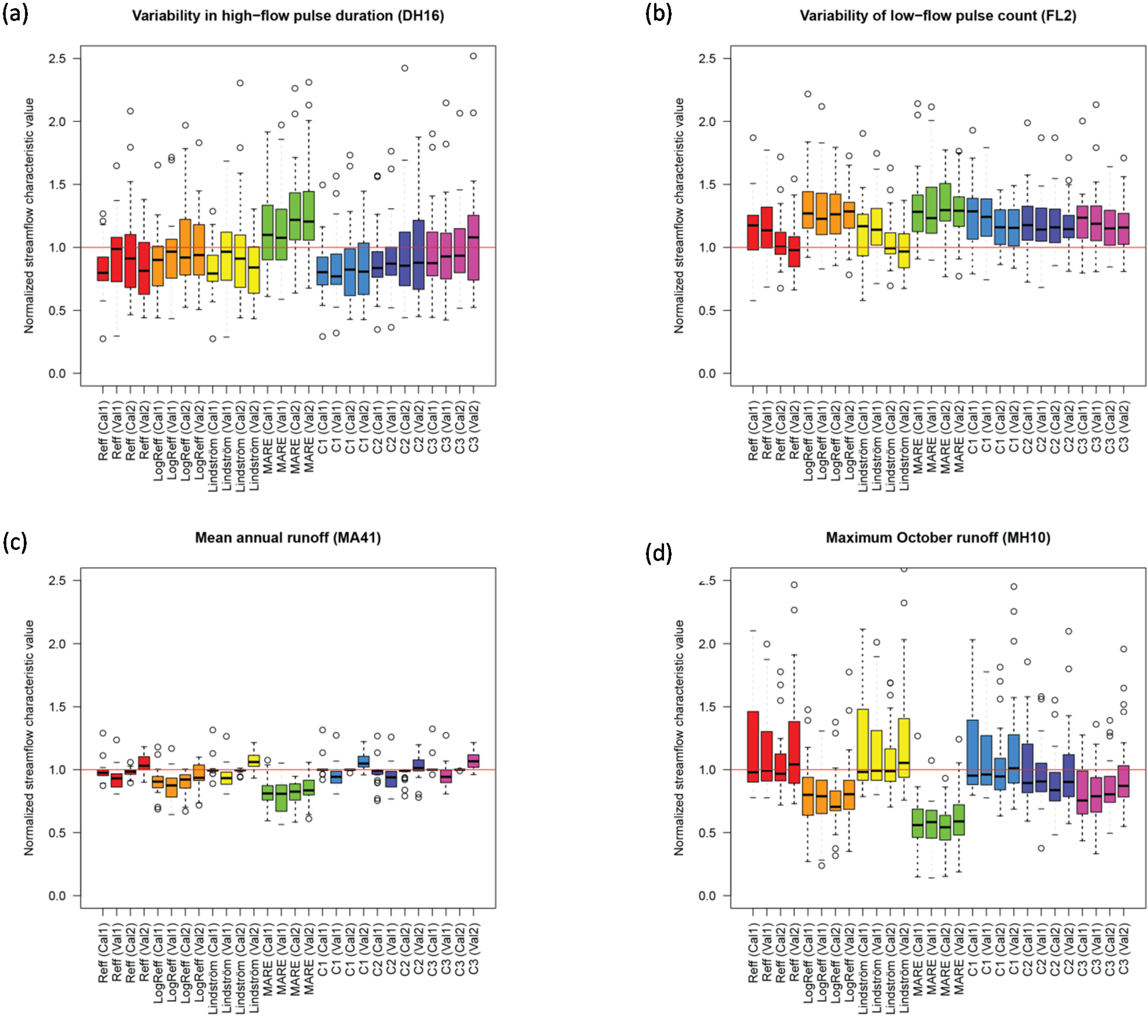
The agreement between observed and simulated flow characteristics varied considerably among the different catchments (Figure 3). Each plot contains 28 boxplots (one for each combination of an objective function, time period and calibration or validation). Each boxplot is based on 27 values (one value per catchment), which were normalized by dividing the median streamflow characteristic value based on simulated runoff by the corresponding streamflow characteristic value computed based on the observed runoff time series. The spread between the different catchments is much smaller for the streamflow characteristic MA41 (mean annual runoff) than for the other flow characteristics. Except for the criteria LogReff and MARE, MA41 was reproduced well for both calibration periods, whereas values were slightly underestimated when being validated on period 1 and slightly overestimated when validated on period 2. Both MA41 (mean annual runoff) and MH10 (maximum October runoff) were reproduced less well for parameter sets derived by calibration based on the criteria LogReff and MARE, both of which are more sensitive to low flow conditions than the other criteria.

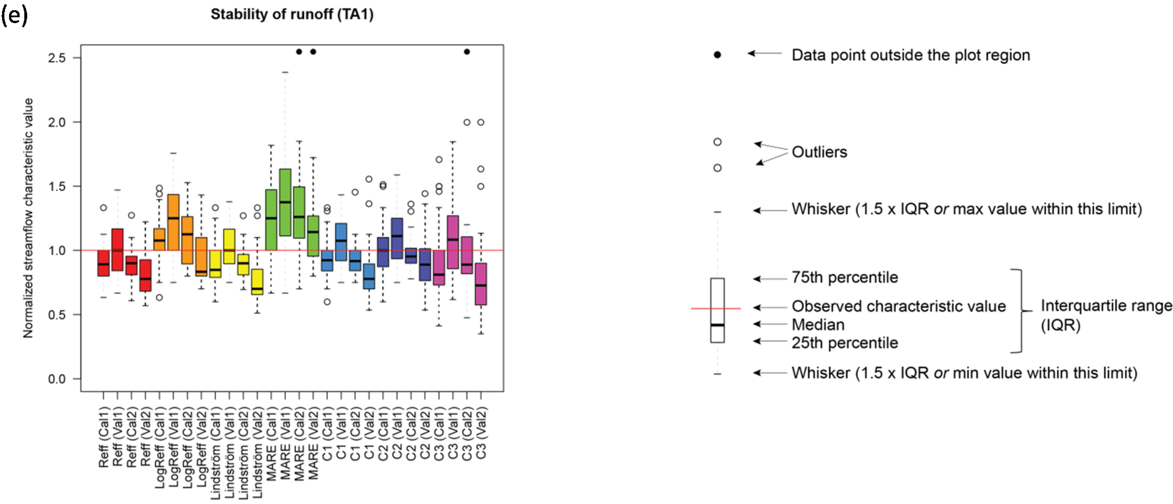
Figure 3. Normalized median flow characteristic values for five different flow characteristics: (a) DH16 (Variability in high-flow pulse duration); (b) FL2 (Variability of low-flow pulse count); (c) MA41 (Mean annual runoff); (d) MH10 (Maximum October runoff) and (e) TA1 (Stability of runoff). Each color corresponds to an objective function. Per objective function, the four boxplots represent (from left to right) calibration period 1 (Cal1), validation period 1 (Val1), calibration period 2 (Cal2) and validation period 2 (Val2). Each boxplot is based on 27 normalized median flow characteristic values, one value for each of the 27 catchments. Medians were computed over 100 runs per catchment. Normalization was carried out by dividing the median values by the corresponding observed flow characteristic value.

Figure 3. Normalized median flow characteristic values for five different flow characteristics: (a) DH16 (Variability in high-flow pulse duration); (b) FL2 (Variability of low-flow pulse count); (c) MA41 (Mean annual runoff); (d) MH10 (Maximum October runoff) and (e) TA1 (Stability of runoff). Each color corresponds to an objective function. Per objective function, the four boxplots represent (from left to right) calibration period 1 (Cal1), validation period 1 (Val1), calibration period 2 (Cal2) and validation period 2 (Val2). Each boxplot is based on 27 normalized median flow characteristic values, one value for each of the 27 catchments. Medians were computed over 100 runs per catchment. Normalization was carried out by dividing the median values by the corresponding observed flow characteristic value.

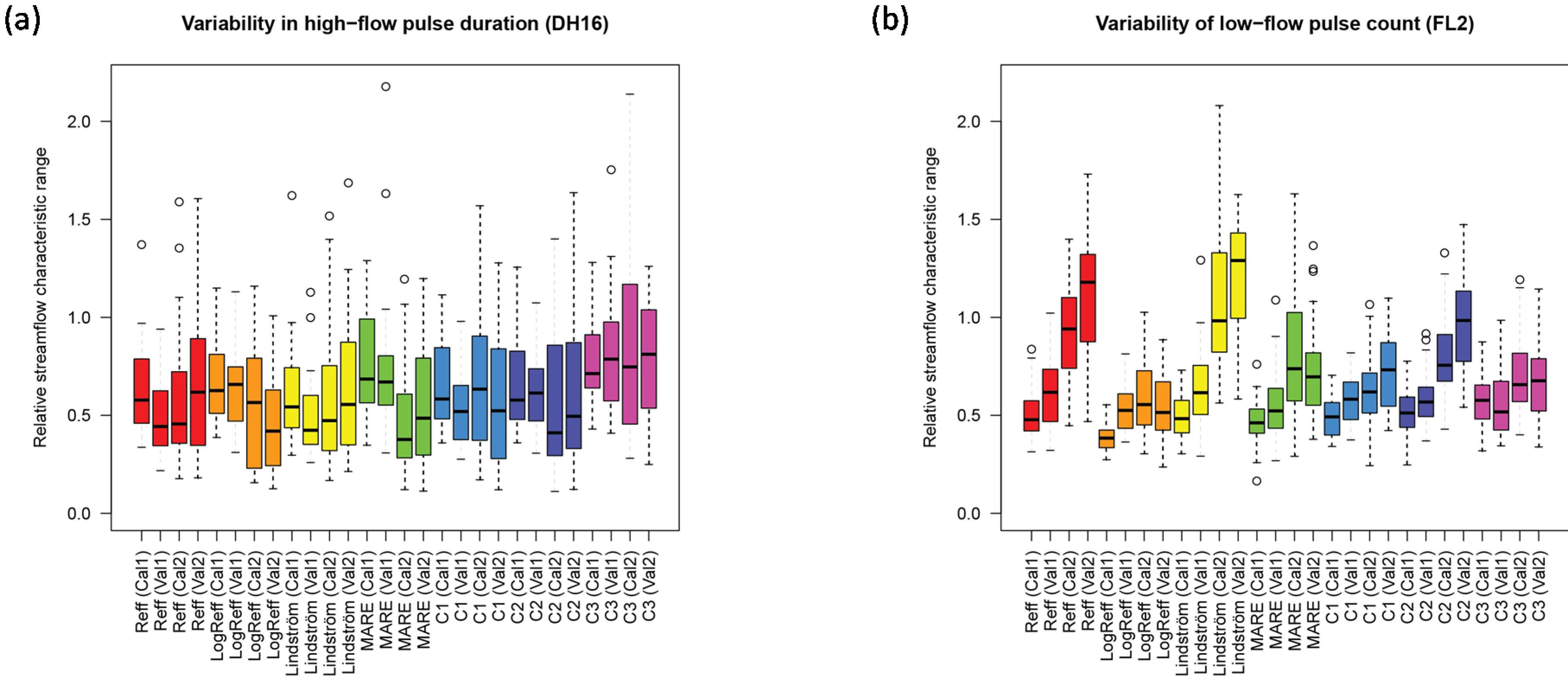
The distribution of the 27 relative ranges (per catchment—Dividing the range over the 100 runs per catchment by the range over the 27 median catchment values) is a measure for the consistency over the different catchments (Figure 4). While for some cases there was a low variation (indicated by narrow distributions of relative range), for many cases a considerable variation was observed. For calibrations based on the Nash-Sutcliffe efficiency, for instance, the median relative range varied from around 0.1 for MA41 (mean annual runoff) to above 1 for FL2 (variability of low-flow pulse count).

Figure 4. Relative ranges as a measure for parameter uncertainty for streamflow characteristics (a) DH16 (Variability in high-flow pulse duration); (b) FL2 (Variability of low-flow pulse count); (c) MA41 (Mean annual runoff); (d) MH10 (Maximum October runoff) and (e) TA1 (Stability of runoff). Each color corresponds to an objective function. Per objective function, the four boxplots represent (from left to right) calibration period 1 (Cal1), validation period 1 (Val1), calibration period 2 (Cal2) and validation period 2 (Val2). Each boxplot is based on 27 values, one value for each of the 27 catchments. Relative ranges were computed by dividing the range over the 100 runs per catchment by the range over the 27 median catchment values. Note that the Mean annual runoff (MA41) has been plotted on a different scale.

Figure 4. Relative ranges as a measure for parameter uncertainty for streamflow characteristics (a) DH16 (Variability in high-flow pulse duration); (b) FL2 (Variability of low-flow pulse count); (c) MA41 (Mean annual runoff); (d) MH10 (Maximum October runoff) and (e) TA1 (Stability of runoff). Each color corresponds to an objective function. Per objective function, the four boxplots represent (from left to right) calibration period 1 (Cal1), validation period 1 (Val1), calibration period 2 (Cal2) and validation period 2 (Val2). Each boxplot is based on 27 values, one value for each of the 27 catchments. Relative ranges were computed by dividing the range over the 100 runs per catchment by the range over the 27 median catchment values. Note that the Mean annual runoff (MA41) has been plotted on a different scale.

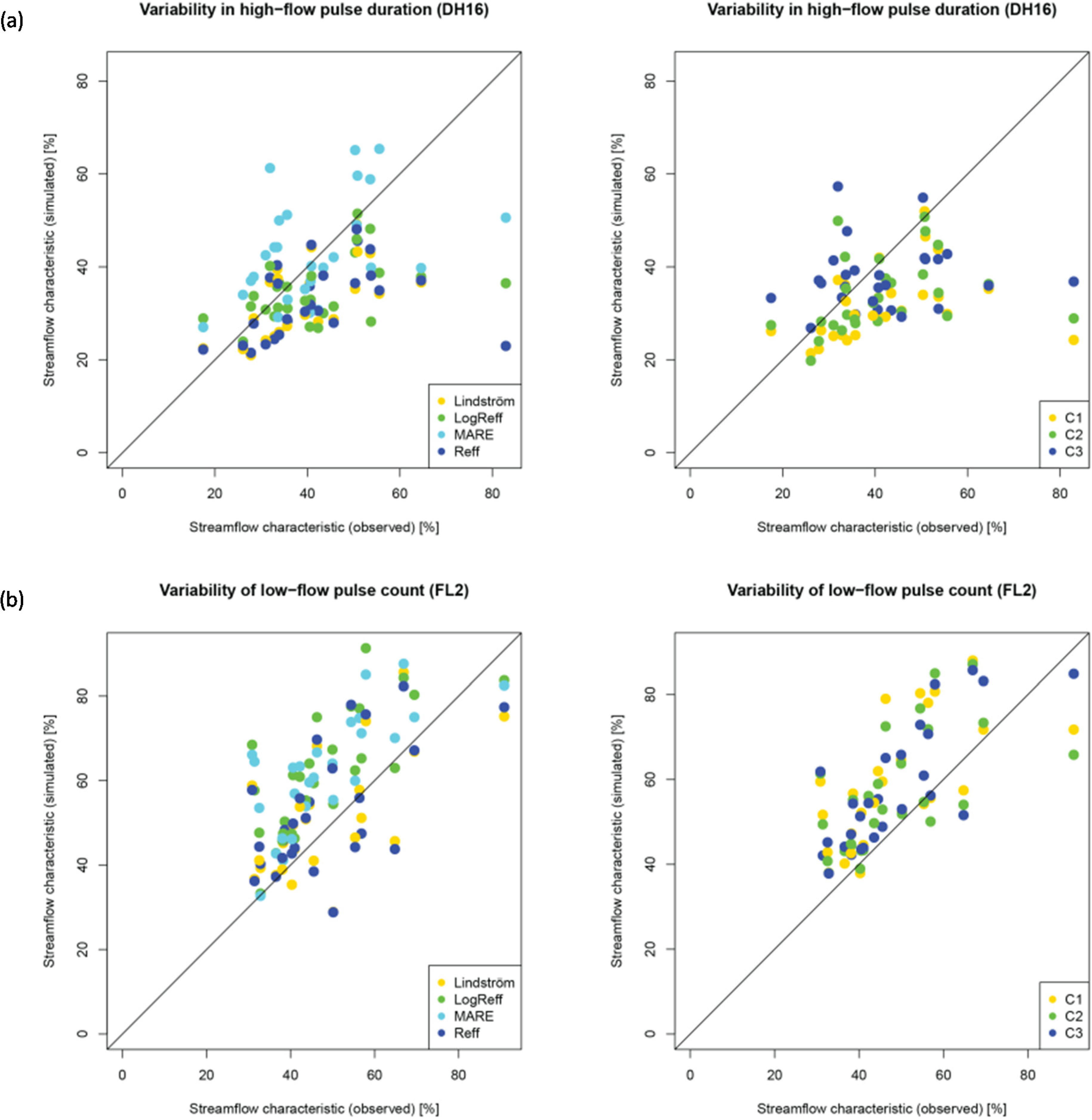
Agreement among the different streamflow characteristics and the different objective functions varied considerably (Figure 5). Comparison of streamflow characteristics based on observed runoff series against the medians of those obtained from simulated time series allows evaluating the agreement in relation to the variation between catchments. These scatter plots show that the agreement varied considerably among both the different streamflow characteristics and the different objective functions. While only plots with flow characteristics calculated for the first calibration period are shown, results were similar for the other calibration and validation periods. The performance for all streamflow characteristics and all combinations of calibration/validation periods were evaluated using the Spearman rank correlation coefficients (Table 6), which evaluates how well the relative ranking of the indices between the catchments is captured, and the model efficiencies (Table 7), which evaluate how well the exact values were predicted. Typically, the values were similar for periods 1 and 2, when the parameterizations obtained by calibration for the respective period were used, resulting in a median difference of 0.015 for the Spearman Rank correlation and 0.0855 for NSE. In general, results are expected to be poorer for the validation period in comparison to the calibration period; however, for the respective validation periods the values were only slightly lower (median difference of −0.0215 (Spearman) and −0.029 (NSE)). This indicates that results were similar for the two periods and were similar when looking at the validation periods. The average median percent error for estimated streamflow characteristics was almost always less than zero, indicating that the objective functions used for model calibration typically underestimated each of the 12 streamflow characteristics being evaluated (Table 8).

Figure 5. Scatterplots for the streamflow characteristics (a) DH16 (Variability in high-flow pulse duration); (b) FL2 (Variability of low-flow pulse count); (c) MA41 (Mean annual runoff); (d) MH10 (Maximum October runoff) and (e) TA1 (Stability of runoff) for calibration period 1. The points represent the median value of all 100 calibration trials in each catchment based on single criteria objective functions (left column) and multi-criteria objective functions (right column).

Figure 5. Scatterplots for the streamflow characteristics (a) DH16 (Variability in high-flow pulse duration); (b) FL2 (Variability of low-flow pulse count); (c) MA41 (Mean annual runoff); (d) MH10 (Maximum October runoff) and (e) TA1 (Stability of runoff) for calibration period 1. The points represent the median value of all 100 calibration trials in each catchment based on single criteria objective functions (left column) and multi-criteria objective functions (right column).

Table 6. Spearman rank correlation coefficients between objective functions (horizontal) and streamflow characteristics (vertical) based on observed respective simulated streamflow (for each group of four values: upper − left = calibration period 1 (Cal1), upper − right = validation period 2 (Val2), lower − left = validation period 1 (Val1), lower − right = calibration period 2 (Cal2)). Colors are ranging from white (for a Spearman rank correlation of 0) to dark green (for a Spearman rank correlation of 1).

	Reff		LogReff		Lindström		MARE		C1		C2		C3
MA41	0.973	0.978	0.930	0.927	0.980	0.983	0.919	0.918	0.980	0.981	0.947	0.928	0.981	0.986
	0.957	0.991	0.929	0.947	0.961	0.998	0.926	0.950	0.961	1.000	0.952	0.979	0.962	1.000
MH10	0.930	0.831	0.874	0.853	0.916	0.837	0.834	0.829	0.941	0.837	0.958	0.874	0.918	0.898
	0.960	0.940	0.862	0.868	0.958	0.934	0.822	0.829	0.957	0.918	0.942	0.903	0.885	0.933
Flowperc	0.796	0.978	0.810	0.986	0.790	0.961	0.814	0.979	0.808	0.980	0.810	0.983	0.685	0.867
	0.778	0.985	0.808	0.996	0.781	0.980	0.804	0.996	0.803	0.995	0.806	0.996	0.683	0.897
RA7	0.736	0.724	0.877	0.885	0.726	0.735	0.888	0.896	0.870	0.873	0.851	0.892	0.696	0.797
	0.756	0.836	0.930	0.930	0.719	0.775	0.848	0.902	0.878	0.919	0.880	0.917	0.744	0.789
DH13	0.977	0.938	0.974	0.948	0.971	0.908	0.960	0.960	0.981	0.945	0.976	0.945	0.926	0.691
	0.955	0.866	0.976	0.937	0.955	0.877	0.964	0.957	0.971	0.910	0.978	0.885	0.871	0.573
TA1	0.972	0.929	0.968	0.943	0.977	0.906	0.947	0.974	0.968	0.884	0.960	0.899	0.875	0.766
	0.936	0.956	0.933	0.966	0.952	0.942	0.884	0.936	0.958	0.948	0.942	0.964	0.904	0.924
FH6	0.943	0.851	0.916	0.906	0.935	0.875	0.728	0.863	0.953	0.916	0.900	0.921	0.569	0.663
	0.926	0.888	0.853	0.931	0.931	0.898	0.634	0.855	0.942	0.930	0.901	0.919	0.498	0.613
FH7	0.948	0.933	0.881	0.889	0.949	0.935	0.810	0.887	0.967	0.945	0.965	0.952	0.688	0.563
	0.927	0.951	0.842	0.889	0.941	0.960	0.763	0.805	0.945	0.967	0.944	0.967	0.480	0.520
MA26	0.849	0.917	0.789	0.906	0.855	0.920	0.704	0.858	0.894	0.923	0.903	0.915	0.631	0.856
	0.752	0.932	0.699	0.894	0.782	0.935	0.672	0.829	0.821	0.933	0.831	0.928	0.381	0.769
DH16	0.534	0.645	0.443	0.662	0.503	0.673	0.402	0.471	0.510	0.745	0.525	0.683	0.145	0.482
	0.429	0.549	0.421	0.654	0.410	0.514	0.346	0.645	0.526	0.659	0.511	0.650	0.094	0.518
FL2	0.521	0.443	0.740	0.628	0.609	0.449	0.734	0.703	0.709	0.602	0.684	0.668	0.755	0.594
	0.548	0.617	0.659	0.604	0.579	0.659	0.641	0.626	0.672	0.711	0.620	0.695	0.616	0.628
TL1	0.477	0.394	0.643	0.520	0.471	0.347	0.612	0.753	0.603	0.330	0.531	0.428	0.574	0.418
	0.407	0.112	0.646	0.546	0.418	0.065	0.623	0.777	0.497	0.362	0.531	0.201	0.600	0.280

Table 6. Spearman rank correlation coefficients between objective functions (horizontal) and streamflow characteristics (vertical) based on observed respective simulated streamflow (for each group of four values: upper − left = calibration period 1 (Cal1), upper − right = validation period 2 (Val2), lower − left = validation period 1 (Val1), lower − right = calibration period 2 (Cal2)). Colors are ranging from white (for a Spearman rank correlation of 0) to dark green (for a Spearman rank correlation of 1).

	Reff		LogReff		Lindström		MARE		C1		C2		C3
MA41	0.973	0.978	0.930	0.927	0.980	0.983	0.919	0.918	0.980	0.981	0.947	0.928	0.981	0.986
	0.957	0.991	0.929	0.947	0.961	0.998	0.926	0.950	0.961	1.000	0.952	0.979	0.962	1.000
MH10	0.930	0.831	0.874	0.853	0.916	0.837	0.834	0.829	0.941	0.837	0.958	0.874	0.918	0.898
	0.960	0.940	0.862	0.868	0.958	0.934	0.822	0.829	0.957	0.918	0.942	0.903	0.885	0.933
Flowperc	0.796	0.978	0.810	0.986	0.790	0.961	0.814	0.979	0.808	0.980	0.810	0.983	0.685	0.867
	0.778	0.985	0.808	0.996	0.781	0.980	0.804	0.996	0.803	0.995	0.806	0.996	0.683	0.897
RA7	0.736	0.724	0.877	0.885	0.726	0.735	0.888	0.896	0.870	0.873	0.851	0.892	0.696	0.797
	0.756	0.836	0.930	0.930	0.719	0.775	0.848	0.902	0.878	0.919	0.880	0.917	0.744	0.789
DH13	0.977	0.938	0.974	0.948	0.971	0.908	0.960	0.960	0.981	0.945	0.976	0.945	0.926	0.691
	0.955	0.866	0.976	0.937	0.955	0.877	0.964	0.957	0.971	0.910	0.978	0.885	0.871	0.573
TA1	0.972	0.929	0.968	0.943	0.977	0.906	0.947	0.974	0.968	0.884	0.960	0.899	0.875	0.766
	0.936	0.956	0.933	0.966	0.952	0.942	0.884	0.936	0.958	0.948	0.942	0.964	0.904	0.924
FH6	0.943	0.851	0.916	0.906	0.935	0.875	0.728	0.863	0.953	0.916	0.900	0.921	0.569	0.663
	0.926	0.888	0.853	0.931	0.931	0.898	0.634	0.855	0.942	0.930	0.901	0.919	0.498	0.613
FH7	0.948	0.933	0.881	0.889	0.949	0.935	0.810	0.887	0.967	0.945	0.965	0.952	0.688	0.563
	0.927	0.951	0.842	0.889	0.941	0.960	0.763	0.805	0.945	0.967	0.944	0.967	0.480	0.520
MA26	0.849	0.917	0.789	0.906	0.855	0.920	0.704	0.858	0.894	0.923	0.903	0.915	0.631	0.856
	0.752	0.932	0.699	0.894	0.782	0.935	0.672	0.829	0.821	0.933	0.831	0.928	0.381	0.769
DH16	0.534	0.645	0.443	0.662	0.503	0.673	0.402	0.471	0.510	0.745	0.525	0.683	0.145	0.482
	0.429	0.549	0.421	0.654	0.410	0.514	0.346	0.645	0.526	0.659	0.511	0.650	0.094	0.518
FL2	0.521	0.443	0.740	0.628	0.609	0.449	0.734	0.703	0.709	0.602	0.684	0.668	0.755	0.594
	0.548	0.617	0.659	0.604	0.579	0.659	0.641	0.626	0.672	0.711	0.620	0.695	0.616	0.628
TL1	0.477	0.394	0.643	0.520	0.471	0.347	0.612	0.753	0.603	0.330	0.531	0.428	0.574	0.418
	0.407	0.112	0.646	0.546	0.418	0.065	0.623	0.777	0.497	0.362	0.531	0.201	0.600	0.280

Table 7. Nash-Sutcliffe efficiencies between objective functions (horizontal) and streamflow characteristics (vertical) based on observed respective simulated streamflow (for each group of four values: upper − left = calibration period 1 (Cal1), upper − right = validation period 2 (Val2), lower − left = validation period 1 (Val1), lower − right = calibration period 2 (Cal2)). Colors are ranging from white (for Nash-Sutcliffe efficiencies of 0 or lower) to dark green (for a Nash-Sutcliffe efficiency of 1).

	Reff		LogReff		Lindström		MARE		C1		C2		C3
MA41	0.917	0.936	0.840	0.881	0.936	0.933	0.584	0.626	0.946	0.939	0.922	0.927	0.949	0.930
	0.858	0.967	0.746	0.835	0.900	0.993	0.490	0.554	0.914	0.999	0.875	0.965	0.916	1.000
MH10	0.848	0.820	−0.627	0.570	0.841	0.796	−3.942	−1.220	0.820	0.871	0.796	0.879	−1.630	0.663
	0.859	0.934	−0.931	0.332	0.874	0.926	−5.692	−2.258	0.848	0.926	0.756	0.850	−1.367	0.667
Flowperc	0.416	0.749	0.611	0.837	0.356	0.660	0.647	0.960	0.463	0.680	0.614	0.804	0.170	0.477
	0.484	0.868	0.569	0.967	0.491	0.820	0.465	0.966	0.538	0.848	0.591	0.939	0.373	0.669
RA7	0.209	0.281	0.071	0.193	0.279	0.370	−0.420	−0.284	−0.043	−0.063	−0.229	−0.197	−9.226	−7.224
	−0.628	−0.230	0.369	0.385	−0.608	−0.277	0.156	0.186	0.276	0.252	0.190	0.231	−5.173	−4.088
DH13	0.372	−0.164	0.884	0.472	−0.601	−1.895	0.910	0.858	0.797	0.522	0.770	0.874	−7.603	−20.044
	0.638	0.427	0.919	0.748	0.437	−0.030	0.814	0.914	0.902	0.813	0.672	0.817	−4.235	−14.891
TA1	0.898	0.432	0.856	0.882	0.829	0.108	0.672	0.803	0.918	0.477	0.886	0.749	0.502	-1.020
	0.863	0.912	0.718	0.845	0.892	0.926	0.548	0.685	0.881	0.974	0.839	0.953	0.806	0.705
FH6	0.709	0.628	−1.354	−0.967	0.660	0.559	−7.331	−4.461	0.513	0.502	0.210	0.282	−3.781	−5.629
	0.714	0.622	−0.788	−0.465	0.717	0.612	−4.768	−3.426	0.736	0.680	0.533	0.522	−2.536	−4.020
FH7	0.746	0.756	−0.440	−1.246	0.585	0.600	−0.752	−1.837	0.769	0.725	0.842	0.820	−13.413	−22.837
	0.813	0.826	0.290	−0.242	0.801	0.820	−0.260	−0.612	0.912	0.930	0.932	0.954	−9.425	−11.728
MA26	0.618	0.849	0.080	0.033	0.582	0.832	−0.418	−1.114	0.789	0.882	0.848	0.872	−4.116	−4.256
	0.331	0.862	0.184	0.320	0.324	0.886	0.178	−0.513	0.500	0.894	0.564	0.878	−1.898	−2.343
DH16	−3.044	−0.329	−3.375	0.050	−3.323	−0.307	−0.463	−0.371	−3.727	−0.006	−2.768	0.192	−3.474	−0.562
	−0.937	−0.182	−2.056	0.186	−1.012	−0.234	−1.025	0.006	−1.535	−0.092	−1.562	0.119	−2.785	−0.309
FL2	0.118	−1.176	−0.469	−1.557	0.201	−0.931	−0.556	−1.448	−0.266	−0.827	−0.167	−1.773	0.139	−0.948
	−0.040	−1.198	−0.530	−1.841	0.056	−1.123	−0.759	−1.703	−0.203	−0.409	−0.132	−1.246	-0.104	−1.018
TL1	−0.376	−4.676	−0.211	−3.016	−0.310	−5.502	−0.361	−2.672	−0.017	−4.483	−0.196	−4.053	−0.023	−2.708
	−0.505	−4.322	−0.250	−3.892	−0.518	−4.338	−0.557	−2.218	−0.400	−4.503	−0.489	−5.932	0.021	−3.529

Table 7. Nash-Sutcliffe efficiencies between objective functions (horizontal) and streamflow characteristics (vertical) based on observed respective simulated streamflow (for each group of four values: upper − left = calibration period 1 (Cal1), upper − right = validation period 2 (Val2), lower − left = validation period 1 (Val1), lower − right = calibration period 2 (Cal2)). Colors are ranging from white (for Nash-Sutcliffe efficiencies of 0 or lower) to dark green (for a Nash-Sutcliffe efficiency of 1).

	Reff		LogReff		Lindström		MARE		C1		C2		C3
MA41	0.917	0.936	0.840	0.881	0.936	0.933	0.584	0.626	0.946	0.939	0.922	0.927	0.949	0.930
	0.858	0.967	0.746	0.835	0.900	0.993	0.490	0.554	0.914	0.999	0.875	0.965	0.916	1.000
MH10	0.848	0.820	−0.627	0.570	0.841	0.796	−3.942	−1.220	0.820	0.871	0.796	0.879	−1.630	0.663
	0.859	0.934	−0.931	0.332	0.874	0.926	−5.692	−2.258	0.848	0.926	0.756	0.850	−1.367	0.667
Flowperc	0.416	0.749	0.611	0.837	0.356	0.660	0.647	0.960	0.463	0.680	0.614	0.804	0.170	0.477
	0.484	0.868	0.569	0.967	0.491	0.820	0.465	0.966	0.538	0.848	0.591	0.939	0.373	0.669
RA7	0.209	0.281	0.071	0.193	0.279	0.370	−0.420	−0.284	−0.043	−0.063	−0.229	−0.197	−9.226	−7.224
	−0.628	−0.230	0.369	0.385	−0.608	−0.277	0.156	0.186	0.276	0.252	0.190	0.231	−5.173	−4.088
DH13	0.372	−0.164	0.884	0.472	−0.601	−1.895	0.910	0.858	0.797	0.522	0.770	0.874	−7.603	−20.044
	0.638	0.427	0.919	0.748	0.437	−0.030	0.814	0.914	0.902	0.813	0.672	0.817	−4.235	−14.891
TA1	0.898	0.432	0.856	0.882	0.829	0.108	0.672	0.803	0.918	0.477	0.886	0.749	0.502	-1.020
	0.863	0.912	0.718	0.845	0.892	0.926	0.548	0.685	0.881	0.974	0.839	0.953	0.806	0.705
FH6	0.709	0.628	−1.354	−0.967	0.660	0.559	−7.331	−4.461	0.513	0.502	0.210	0.282	−3.781	−5.629
	0.714	0.622	−0.788	−0.465	0.717	0.612	−4.768	−3.426	0.736	0.680	0.533	0.522	−2.536	−4.020
FH7	0.746	0.756	−0.440	−1.246	0.585	0.600	−0.752	−1.837	0.769	0.725	0.842	0.820	−13.413	−22.837
	0.813	0.826	0.290	−0.242	0.801	0.820	−0.260	−0.612	0.912	0.930	0.932	0.954	−9.425	−11.728
MA26	0.618	0.849	0.080	0.033	0.582	0.832	−0.418	−1.114	0.789	0.882	0.848	0.872	−4.116	−4.256
	0.331	0.862	0.184	0.320	0.324	0.886	0.178	−0.513	0.500	0.894	0.564	0.878	−1.898	−2.343
DH16	−3.044	−0.329	−3.375	0.050	−3.323	−0.307	−0.463	−0.371	−3.727	−0.006	−2.768	0.192	−3.474	−0.562
	−0.937	−0.182	−2.056	0.186	−1.012	−0.234	−1.025	0.006	−1.535	−0.092	−1.562	0.119	−2.785	−0.309
FL2	0.118	−1.176	−0.469	−1.557	0.201	−0.931	−0.556	−1.448	−0.266	−0.827	−0.167	−1.773	0.139	−0.948
	−0.040	−1.198	−0.530	−1.841	0.056	−1.123	−0.759	−1.703	−0.203	−0.409	−0.132	−1.246	-0.104	−1.018
TL1	−0.376	−4.676	−0.211	−3.016	−0.310	−5.502	−0.361	−2.672	−0.017	−4.483	−0.196	−4.053	−0.023	−2.708
	−0.505	−4.322	−0.250	−3.892	−0.518	−4.338	−0.557	−2.218	−0.400	−4.503	−0.489	−5.932	0.021	−3.529

Table 8. Median percent error for streamflow characteristics by model objective function for calibration period 1 (Cal1).

Objective Function	MA41	MH10	RA7	TA1	DH13	FH7	FH6	FL2	MA26	DH16	TL1	E85	Average Median Error (Percent)
Lindström	−0.6	−1.8	−25.0	−15.2	−18.1	−23.0	−12.0	16.8	9.1	−20.8	3.7	19.1	−5.6
LogReff	−9.5	−20.0	−50.0	7.7	−9.5	−37.5	−27.0	26.9	−7.3	−10.0	4.8	15.2	−9.7
MARE	−18.9	−44.0	−57.1	25.0	−7.4	−44.4	−41.4	28.2	−19.6	9.9	5.5	−7.3	−14.3
Reff	−2.5	−2.1	−18.2	−10.8	−14.7	−20.0	−12.0	17.5	9.8	−20.2	4.2	9.8	−4.9
C1	0.0	−4.8	−50.0	−7.7	−13.1	−19.0	−14.1	28.6	4.9	−19.7	3.4	29.9	−5.1
C2	−0.8	−10.6	−42.9	0.0	−7.5	−14.0	−18.2	17.7	2.2	−16.4	4.0	13.2	−6.1
C3	0.0	−24.5	−44.4	−18.9	−18.9	−69.3	−37.6	23.6	−28.1	−12.5	3.4	24.1	−16.9
Average Median Percent Error	−4.6	−15.4	−41.1	−2.8	−12.7	−32.5	−23.2	22.8	−4.2	−12.8	4.1	14.9	–

Table 8. Median percent error for streamflow characteristics by model objective function for calibration period 1 (Cal1).

Objective Function	MA41	MH10	RA7	TA1	DH13	FH7	FH6	FL2	MA26	DH16	TL1	E85	Average Median Error (Percent)
Lindström	−0.6	−1.8	−25.0	−15.2	−18.1	−23.0	−12.0	16.8	9.1	−20.8	3.7	19.1	−5.6
LogReff	−9.5	−20.0	−50.0	7.7	−9.5	−37.5	−27.0	26.9	−7.3	−10.0	4.8	15.2	−9.7
MARE	−18.9	−44.0	−57.1	25.0	−7.4	−44.4	−41.4	28.2	−19.6	9.9	5.5	−7.3	−14.3
Reff	−2.5	−2.1	−18.2	−10.8	−14.7	−20.0	−12.0	17.5	9.8	−20.2	4.2	9.8	−4.9
C1	0.0	−4.8	−50.0	−7.7	−13.1	−19.0	−14.1	28.6	4.9	−19.7	3.4	29.9	−5.1
C2	−0.8	−10.6	−42.9	0.0	−7.5	−14.0	−18.2	17.7	2.2	−16.4	4.0	13.2	−6.1
C3	0.0	−24.5	−44.4	−18.9	−18.9	−69.3	−37.6	23.6	−28.1	−12.5	3.4	24.1	−16.9
Average Median Percent Error	−4.6	−15.4	−41.1	−2.8	−12.7	−32.5	−23.2	22.8	−4.2	−12.8	4.1	14.9	–

4. Discussion

In the absence of observed data, environmental flow studies necessarily rely on some form of streamflow estimation to model the response of aquatic ecology to alteration of the streamflow regime. Knight et al. [23] and Murphy et al. [8] raised the question of validity and began evaluation of model accuracies for predicting known ecologically-relevant streamflow characteristics. Murphy et al. [8] and Shrestha et al. [9] highlight that typical calibration approaches, often focused on daily, monthly, or annual mean values, are inadequate when predicting more subtle aspects of the flow regime. An increasing body of work is making use of statistical modeling approaches to address hydrologic and hydro-ecological questions [5,7,43,44,45]. However, as already stated by Murphy et al. [8] and Shrestha et al. [9], runoff models have advantages as well as limitations, particularly in regard to developing streamflow time series reflecting land cover, human population, or climatic projections. As such, runoff models should be closely evaluated to better understand if the calibration approaches and predictive accuracies yield results amenable to their end use.

While the HBV-light model was used in this study, there is little reason to assume that results would be discernibly different if another calibrated runoff model were used. Partly this reflects the fact that most mechanistic runoff models are fundamentally similar in concept and application, using more or less the same or similar routines. Fundamentally, if calibration is used, the simulated series are fitted to the observed series according to some objective function, and regardless of the specific model being used, this fit does not ensure agreement in all possible aspects of the hydrograph shape.

The accuracy of prediction and appropriateness of calibration is important in the context of environmental flow application as error of predicting flow-regime components will be translated and probably amplified as error in estimating ecological response. A given approach to model calibration will lead to accurate prediction of the runoff with regard to the used objective function measure, however accurate prediction of other aspects may be lacking. For example, Knight et al. [41] (Figure 2) published linear functions representing the 80th quantile upper-bound relationship of specialized insectivore scores to three streamflow characteristics (TA1, FH6, and RA7; see Table 5 for definitions). Following Murphy et al. [8], we use these relations to evaluate the accuracy of streamflow characteristic predictions as well as predicted ecological response based on the seven calibration approaches discussed herein for a single model (catchment 03488000). Using the equations from Knight et al. 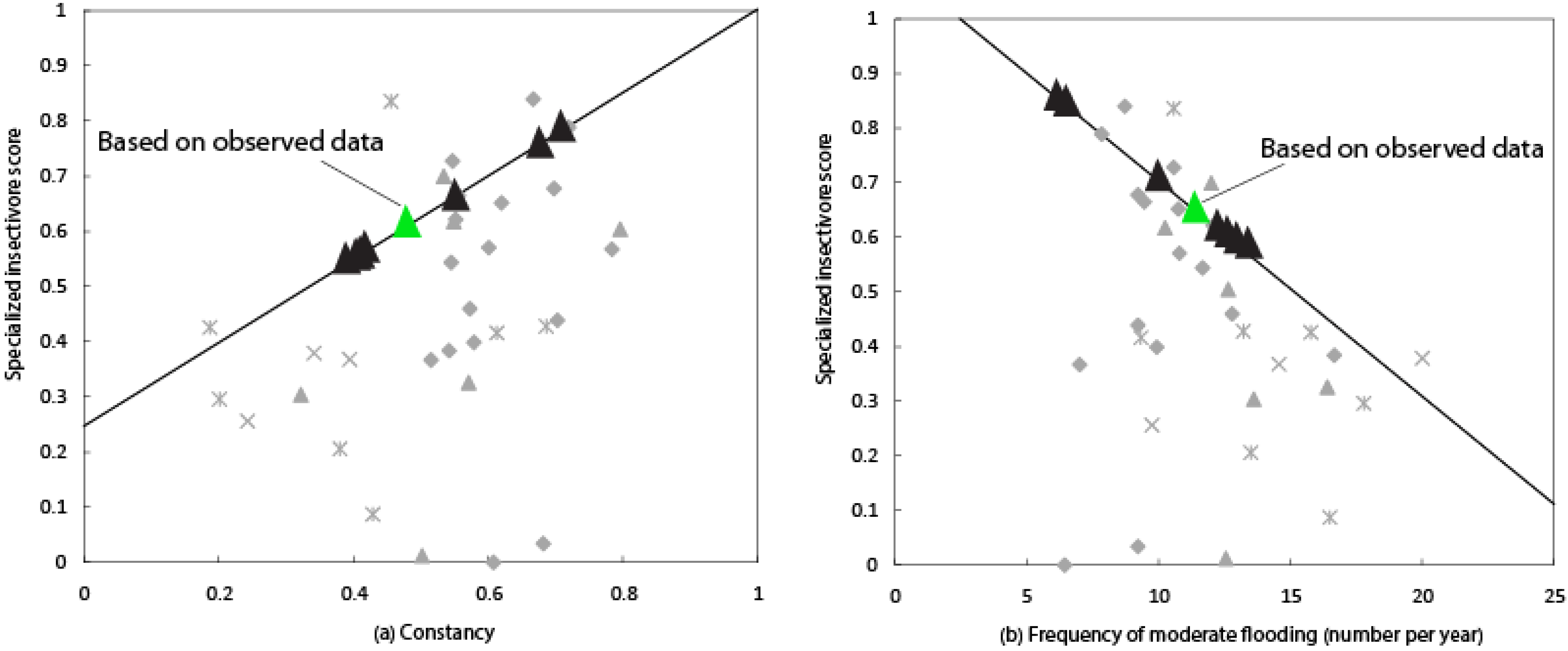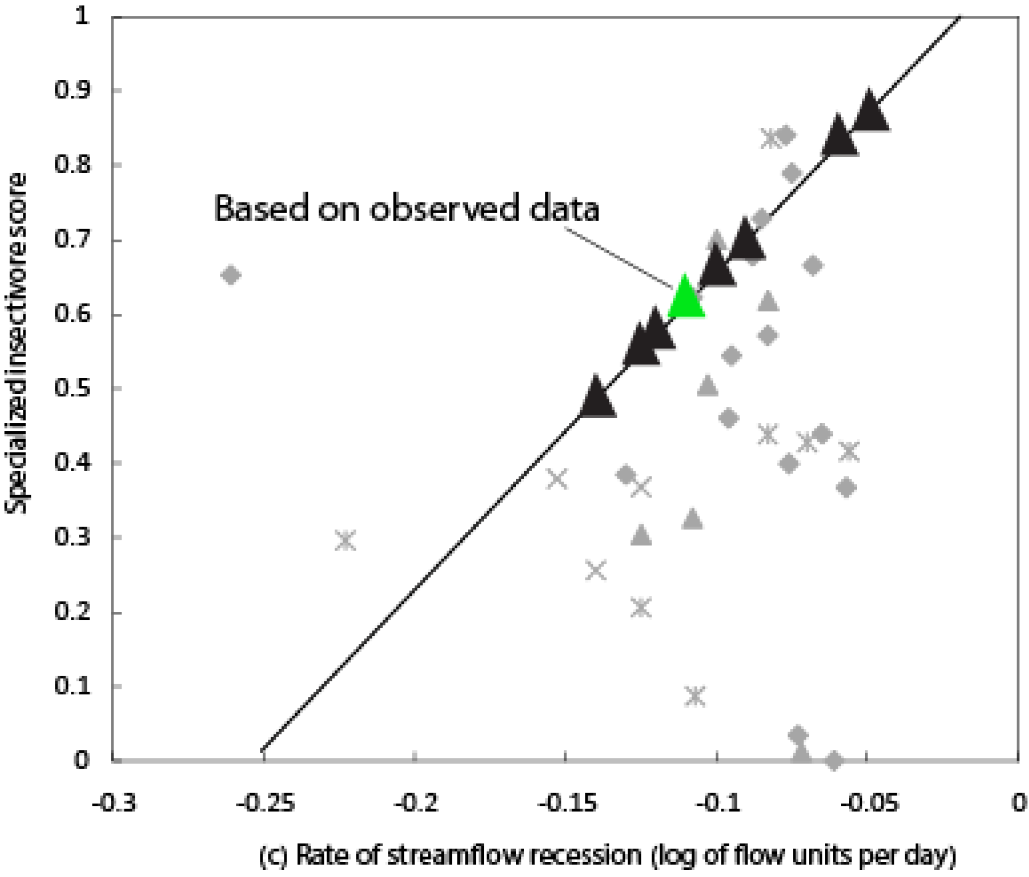[41] and simulated streamflow presented in this paper, values of insectivore scores varied from 0.49 to 0.87 for RA7, 0.53 to 0.8 for TA1, and 0.58 to 0.84 for FH6 (Table 9; Figure 6). While median percent difference error for estimated specialized insectivore score for RA7 was a modest 8.2 percent under the estimate using observed data, individual departures from the observed values ranged from −19.7 to 42.6 percent for RA7, −13.1 to 31.1 percent for TA1, and −10.8 to 29.2 percent for FH6. Model results in this example are similar to those for a regional regression model reported by Murphy et al. [8] (9 percent difference for streamflow characteristic and 16 percent over estimation for insectivore score using HBV-light. Results presented here are considerably different than those for a rainfall-runoff model example from Murphy et al. [8], showing 90 percent overestimated for the same ecological score.

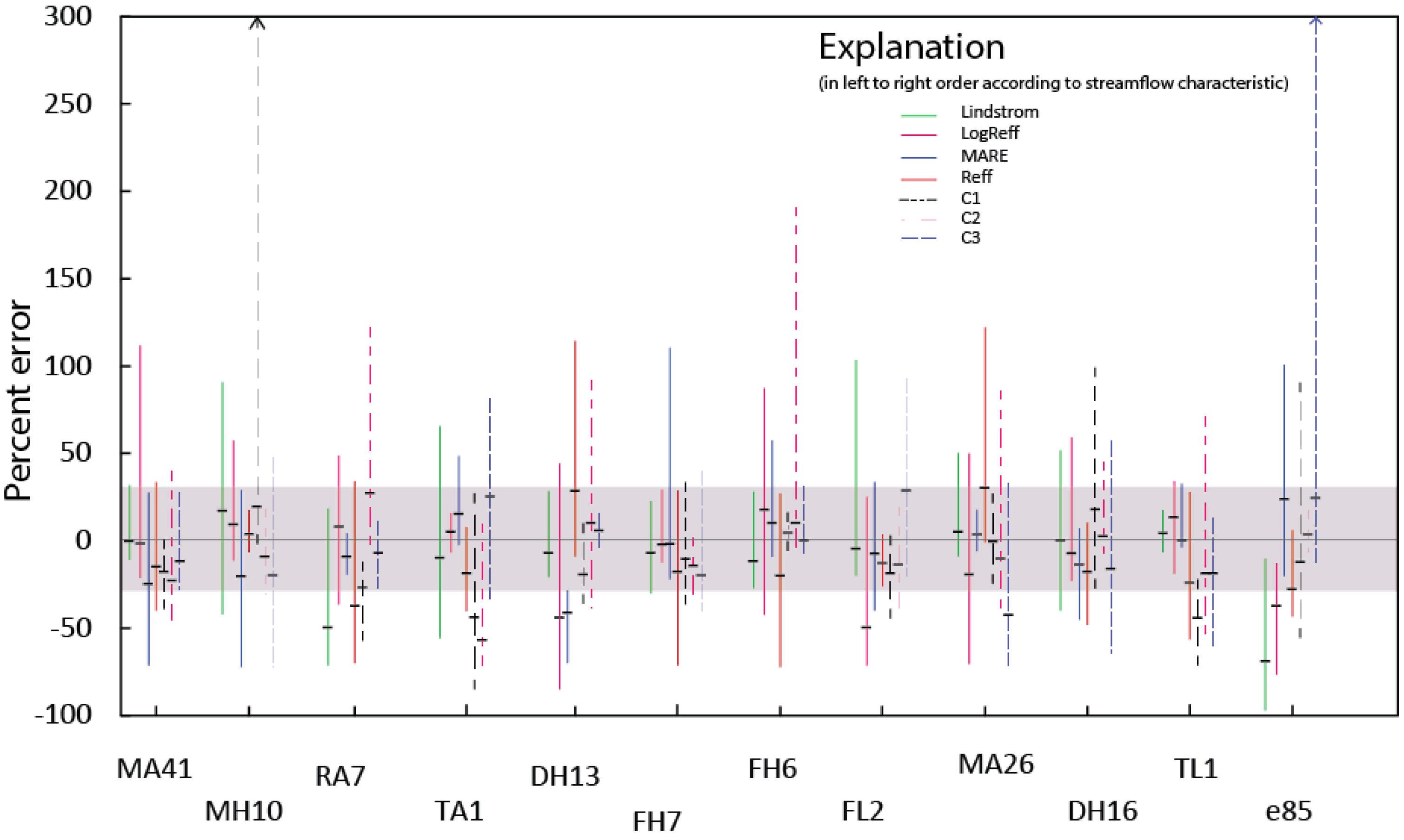
The objective functions used for model calibration resulted overall in an underprediction of the 12 streamflow characteristics being evaluated (Table 8). The general underprediction of the flow characteristics is a result similar to that seen in Murphy et al. [8] where a TOPMODEL application calibrated on mean annual flow was evaluated in the context of predicting the same streamflow characteristics. The median errors presented here are within plus-or-minus 30 percent of observed values, proposed by Kennard et al. [46] as an acceptable band of uncertainty, for 8 to 12 streamflow characteristics (out of 12) depending on the objective function (Figure 7, Table 8). This is in stark contrast to the rainfall runoff model evaluated in Murphy et al. [8] ) where 13 of 19 streamflow characteristics were outside this band. While similar patterns are seen in overall model results, the calibration approaches evaluated in this paper appear to have provided more accurate estimates across the flow regime as defined by these characteristics. These results can be attributed both to the use of 100 parameter sets, which resulted in more robust flow characteristic estimations, and the use of different objective functions. Parameter uncertainty was substantial for many streamflow characteristics depending on which objective function was used. Despite this, high model efficiencies could still be achieved in many cases when using the median of 100 calibration trials as a more robust prediction for streamflow characteristics.

Table 9. Comparison of selected streamflow characteristics based on simulated and observed streamflow time series for a single model location (site 13 (03488000)) and calibration period 1 (Cal1). (TA1, RA7, and FH6, defined in Table 5; values in parentheses represent the specialized insectivore score using the associated streamflow characteristic value based on linear equations presented in Knight et al. [41], Figure 2; hydro, percent error for streamflow characteristic derived from simulated and observed streamflow time series; eco, percent error for specialized insectivore score based on streamflow characteristic derived from simulated and observed streamflow time series).

Objective Function (see Table 3 for Definitions)	RA7		Percent Error	TA1		Percent Error	FH6		Percent Error
	Simulated	Observed	Hydro/Eco	Simulated	Observed	Hydro/Eco	Simulated	Observed	Hydro/Eco
Lindström	0.14 (0.49)		27.3/−19.7	0.4 (0.55)		−16.7/−9.8	13 (0.59)		13.4/−9.2
LogReff	0.1 (0.66)		−9.1/8.2	0.67 (0.75)		39.6/23	10.08 (0.7)		−12/7.7
MARE	0.06 (0.83)	0.11 (0.61)	−45.5/36.1	0.73 (0.8)	0.48 (0.61)	52.1/31.1	6.62 (0.84)	11.46 (0.65)	−42.2/29.2
Reff	0.125 (0.55)		13.6/−9.8	0.41 (0.56)		−14.6/−8.2	13.38 (0.58)		16.8/−10.8
C1	0.12 (0.57)		9.1/−6.6	0.43 (0.57)		−10.4/−6.6	12.92 (0.59)		12.7/−9.2
C2	0.09 (0.7)		−18.2/14.8	0.57 (0.68)		18.8/11.5	12.38 (0.62)		8/−4.6
C3	0.05 (0.87)		−54.5/42.6	0.38 (0.53)		−20.8/−13.1	6.54 (0.84)		−42.9/29.2

Table 9. Comparison of selected streamflow characteristics based on simulated and observed streamflow time series for a single model location (site 13 (03488000)) and calibration period 1 (Cal1). (TA1, RA7, and FH6, defined in Table 5; values in parentheses represent the specialized insectivore score using the associated streamflow characteristic value based on linear equations presented in Knight et al. [41], Figure 2; hydro, percent error for streamflow characteristic derived from simulated and observed streamflow time series; eco, percent error for specialized insectivore score based on streamflow characteristic derived from simulated and observed streamflow time series).

Objective Function (see Table 3 for Definitions)	RA7		Percent Error	TA1		Percent Error	FH6		Percent Error
	Simulated	Observed	Hydro/Eco	Simulated	Observed	Hydro/Eco	Simulated	Observed	Hydro/Eco
Lindström	0.14 (0.49)		27.3/−19.7	0.4 (0.55)		−16.7/−9.8	13 (0.59)		13.4/−9.2
LogReff	0.1 (0.66)		−9.1/8.2	0.67 (0.75)		39.6/23	10.08 (0.7)		−12/7.7
MARE	0.06 (0.83)	0.11 (0.61)	−45.5/36.1	0.73 (0.8)	0.48 (0.61)	52.1/31.1	6.62 (0.84)	11.46 (0.65)	−42.2/29.2
Reff	0.125 (0.55)		13.6/−9.8	0.41 (0.56)		−14.6/−8.2	13.38 (0.58)		16.8/−10.8
C1	0.12 (0.57)		9.1/−6.6	0.43 (0.57)		−10.4/−6.6	12.92 (0.59)		12.7/−9.2
C2	0.09 (0.7)		−18.2/14.8	0.57 (0.68)		18.8/11.5	12.38 (0.62)		8/−4.6
C3	0.05 (0.87)		−54.5/42.6	0.38 (0.53)		−20.8/−13.1	6.54 (0.84)		−42.9/29.2

Figure 6. Example of an ecological flow application by comparison of estimated values for three streamflow characteristics for site 13 (03488000) (Table 1, Figure 1) and calibration period 1 (Cal1). (a) Constancy; (b) Frequency of moderate flooding (number per year) and (c) Rate of streamflow recession (log of flow units per day). Black triangles represent model estimated values based on the seven objective functions. Green triangle represents streamflow characteristics based on observed data. Values for RA7 (Rate of streamflow recession) were multiplied by negative 1 to convert values to those in the original analysis. Thin black lines represent 80th percentile quantile regression lines based on the 33 data point (grayed) in the background used by Knight et al. [41]. (Figure modified from Knight et al. [41]).

Figure 6. Example of an ecological flow application by comparison of estimated values for three streamflow characteristics for site 13 (03488000) (Table 1, Figure 1) and calibration period 1 (Cal1). (a) Constancy; (b) Frequency of moderate flooding (number per year) and (c) Rate of streamflow recession (log of flow units per day). Black triangles represent model estimated values based on the seven objective functions. Green triangle represents streamflow characteristics based on observed data. Values for RA7 (Rate of streamflow recession) were multiplied by negative 1 to convert values to those in the original analysis. Thin black lines represent 80th percentile quantile regression lines based on the 33 data point (grayed) in the background used by Knight et al. [41]. (Figure modified from Knight et al. [41]).

Figure 7. Minimum, maximum, and median percent errors according to objective function and streamflow characteristic for calibration period 1 (Cal1). Each vertical bar is based on the median error for the 27 catchments. The gray band in the center of the figure represents ±30 percent difference [46] Vertical bars with arrows indicate the maximum percent error exceeded the axis scale.

Figure 7. Minimum, maximum, and median percent errors according to objective function and streamflow characteristic for calibration period 1 (Cal1). Each vertical bar is based on the median error for the 27 catchments. The gray band in the center of the figure represents ±30 percent difference [46] Vertical bars with arrows indicate the maximum percent error exceeded the axis scale.

While the low average median percentage error would indicate a good performance with regard to the estimated flow characteristics, the scatter plots and computed Nash-Sutcliffe efficiencies and Spearman rank correlations reveal a slightly different picture. Spearman rank correlations were rather high for many of the objective functions and streamflow characteristics. For many of those objective function and flow characteristic combinations, however, Nash-Sutcliffe efficiencies were much lower. This shows that, although a clear bias might be observed in the predicted streamflow characteristic values, the order between the catchments was preserved quite well. In practice it might be more important to determine how well the flow characteristics are reproduced relative to the variation among catchments in the region than to determine the relative error value. When evaluating the scatter plots (Figure 5), low values of the Nash-Sutcliffe efficiencies indicated that the represented variability was relatively low, and the low Spearman rank correlations indicated that some flow characteristics that were not similar on a ranking scale were estimated correctly for the different catchments.

Considering individual streamflow characteristics, a pattern in predictive accuracy is evident. Most notably, streamflow characteristics that reflect average conditions (MA41, MA26, TA1, and TL1) were predicted quite well, with average median percent errors ranging from 2.8 to 4.6 percent absolute (Table 8). However, for some of these characteristics, especially TL1, the relative variation of the simulated values among the catchments were rather poor (Table 6 and Table 7). Aspects of the hydrograph representative of high-flow conditions (MH10, FH7, FH6, DH13, DH16, and RA7) were underpredicted consistently (between 12.7 and 41.1 percent), with individual model calibrations underpredicting values up to 70 percent under observed. Low-flow characteristics were overpredicted (FL2 and E85) by 22.8 and 14.9 percent respectively. This appears to indicate that the model, regardless of calibration, may be retaining water during high-flow periods and allowing it to release during low-flow periods. The considerable underprediction of RA7 (rate of streamflow recession) indicates that higher flow events receded at a slower rate, which is suggestive of water stored in groundwater, and subsequently abundant groundwater discharge. The underprediction of RA7 and overprediction of low-flow characteristics are complementary.

MA41 (mean annual runoff) was predicted extremely well, particularly when using those calibrations where the objective function included the volume error as criterion, which is expected as this criterion is equivalent to the mean annual runoff. Predictions of MA41 also performed quite well when calibrated using the Nash-Sutcliffe efficiency. This performance might be attributed to the sensitivity of the Nash-Sutcliffe efficiency for high flows, which could reduce the error in the estimation of mean annual runoff. As noted by Murphy et al. [8], inclusion of ecological flow characteristics as criteria in calibrations may yield better simulations.

5. Conclusions

The accuracy of simulated runoff resulting from seven objective functions was evaluated in this paper by comparing streamflow characteristics based on observed and predicted streamflow time series. While the ultimate goal is to produce the most accurate simulated streamflow time series at ungauged catchments based on the transfer of calibrated parameter sets from gauged to ungauged catchments, the comparison in this study addresses an important part of the total uncertainty, namely the uncertainty related to the prediction accuracy specific streamflow characteristics that were not part of the calibration routine. The primary conclusion is that good model performance in terms of objective functions, such as the frequently used Nash-Sutcliffe model efficiency, does not ensure that all flow characteristics computed from these simulations will correspond to those derived from observed runoff. This is an important consideration that is often overlooked by users of model output who use simulated time series for various analyses, supporting resource allocation decisions, or establishing flow policy. While expecting simulated runoff series to agree with the observed in all possible aspects is unreasonable, this analysis serves as a further reminder of the substantial errors possible, using ecological flow characteristics as the example.

Two novel approaches were used in this study. First, we evaluated the effectiveness of seven objective functions for simulating streamflow time series and subsequent streamflow characteristic calculations. This allowed for critical examination of the importance of the objective function choice, as results differed substantially among objective functions. Results indicate there was no single best calibration strategy, but not surprisingly, different strategies provided better predictions for different streamflow characteristics. However, there was some indication that the combined objective functions, which evaluate the runoff simulations in different aspects, might be generally more suitable across a range of flow characteristics. Second, parameter uncertainty was explicitly considered by using the combination of 100 different equally possible parameter sets for each calibration trial instead of the typical single optimal calibrated parameter set. Our results confirmed the value of this approach by showing that different parameter sets can be similar with respect to the objective function used (similarity between the Nash-Sutcliffe for example) but differ greatly with respect to other characteristics. We demonstrated that using only one parameter set could result in substantial uncertainties, which can be reduced by using the values based on several parameter sets as more robust estimation.

More research is needed to determine which objective functions are most useful to ensure acceptable simulations of ecological flow characteristics, or other regime-defining characteristics. One suitable approach beyond the objective functions used in this paper might be to include streamflow characteristics of particular interest as objective functions in the calibration. This corresponds to the suggestion to include various hydrological signatures as diagnostic tools [47]. The fact that simulation-based flow characteristics varied largely depending upon which objective functions were used indicates that there is a considerable potential to improve model calibrations by considering specific flow characteristics when evaluating model performance during calibration. While it can be expected that performances improve when a certain streamflow characteristic is explicitly included in the objective function, it is less clear which criteria should be included to ensure acceptable simulations for calculation of streamflow characteristics in general. Further research is therefore motivated to explore which criteria to include in the objective function to obtain streamflow simulations that preserve as many streamflow characteristics as possible.