Article

Evaluating the Effects of Mulch and Irrigation Amount on Soil Water Distribution and Root Zone Water Balance Using HYDRUS-2D

1
State Key Laboratory of Oasis Desert and Ecology, Xinjiang Institute of Ecology and Geography, CAS, Urumqi 830011, China
2
University of Chinese Academy of Sciences, Beijing 100049, China
3
Genetics and Precision Agriculture Research Unit, USDA-ARS, P. O. BOX 5367, 810 Highway 12 East, Mississippi State, MS 39762, USA
4
Xinjiang Monitoring Station of Water and Soil Conservation, Urumqi 830000, China
*
Author to whom correspondence should be addressed.
Water 2015, 7(6), 2622-2640; https://doi.org/10.3390/w7062622
Submission received: 9 February 2015 / Revised: 10 April 2015 / Accepted: 30 April 2015 / Published: 29 May 2015

Abstract

:
Water scarcity is the most critical constraint for sustainable cotton production in Xinjiang Province, northwest China. Drip irrigation under mulch is a major water-saving irrigation method that has been widely practiced for cotton production in Xinjiang. The performance of such an irrigation system should be evaluated for proper design and management. Therefore, a field experiment and a simulation study were conducted to (1) determine a modeling approach that can be applied to manage drip irrigation under mulch for cotton production in this region; and (2) examine the effects of irrigation amount and mulch on soil water distribution and root zone water balance components. In the experiment, four irrigation treatments were used: T1, 166.5 m3; T2, 140.4 m3; T3, 115.4 m3; and T4: 102.3 m3. The HYDRUS-2D model was calibrated, validated, and applied with the data obtained in this experiment. Soil water balance in the 0–70 cm soil profile was simulated. Results indicate that the observed soil water content and the simulated results obtained with HYDRUS-2D are in good agreement. The radius of the wetting pattern, root water uptake, and evaporation decreased as the amount of irrigation was reduced from T1 to T4, while a lot of stored soil water in the root zone was utilized and a huge amount of water was recharged from the layer below 70 cm to compensate for the decrease in irrigation amount. Mulch significantly reduced evaporation by 11.7 mm and increased root water uptake by 11.2 mm. Our simulation study suggests that this model can be applied to provide assistance in designing drip irrigation systems and developing irrigation strategies.

1. Introduction

The Aksu Region, located in southern Xinjiang, is one of the major areas in China that produces cotton. The main climate feature in this arid region is the extremely high ratio of evaporation to precipitation. Water scarcity is one of the most critical constraints for sustainable cotton production. Drip irrigation under mulch is considered as the most efficient water-saving method because this system can uniformly distribute water, accurately control the amount of applied water, and reduce evaporation [1,2,3]. Hence, this method is widely practiced in semi-arid and arid regions [3,4]. In Xinjiang, drip irrigation under mulch is the main water-saving irrigation method and has been applied to cotton cropping systems since 1996. The area of drip-irrigated farmlands reached 15.3 million ha in 2009 [5].
Considerable progress has been made to understand water flow, solute transport, and root water uptake under drip irrigation covered by mulch. The characteristics of cotton root distribution under different amounts of irrigation have been studied [5,6,7]. Fang et al. [8] reported that cotton root is mainly distributed in the 0–40 cm soil layer, and its biomass in the deep soil layer increases with the decrease in irrigation amount. Yan et al. [9] determined a significant correlation between cotton root length density and biomass. According to their experiment results, maximum cotton production was 6360.8 kg·ha1, which corresponds to an irrigation amount of 3464.4 m3·ha−1 [9,10]. The distribution of water and salt affected by drip irrigation under mulch is also a critical issue that has been studied in various experiments [1,11,12,13,14,15,16,17].
However, the effects of drip irrigation under mulch on soil water movement and root zone water balance components have not been fully studied. Plastic mulch is an important factor that influences soil moisture, soil temperature, and surface microclimate [18]. Moreover, several studies have indicated that plastic mulch has a greater effect on soil water balance and ultimately improves water use efficiency [19,20,21]. Thus, the effects of mulch on soil moisture and root zone water balance under drip irrigation must be examined for the proper design, management, and operation of drip irrigation systems.
Time- and site-specific experiment studies, which have been conducted in this region, can provide information for irrigation management under specific soil–water–plant system and given climate conditions. However, this information may not be applicable to other regions or to the same region in other years because of the high variability of field and climate. Therefore, a model, as a common management tool, is required to guide irrigation practice in different regions. In addition, measuring all soil water balance components in a field experiment is difficult, if not impossible. A modeling approach coupled with field experiments can determine all components of water balance, including root water uptake, drainage, and recharge from low soil profiles.
The soil moisture pattern under drip irrigation has been studied using empirical, analytical, and numerical models in the past decades [22,23,24,25,26,27,28]. HYDRUS-2D is a hydrologic model that simulates water, heat, and solute movements in 2D and 3D variably saturated porous media [29,30]. HYDRUS-2D has been successfully used to model various solute transports under drip irrigation, such as nitrogen leaching, fertigation, and salt accumulation [31,32,33,34,35]. Previous simulation studies [29,36,37,38,39,40] showed that HYDRUS-2D simulations of soil water content are in reasonable agreement with measured values.
In the present work, a field experiment and a simulation study were conducted. The measured data in the field experiment were used to calibrate, validate, and apply the HYDRUS-2D model. Then, the model was used to quantify the effects of mulch and various amounts of drip irrigation on soil water distribution and root zone water balance components, which is essential to evaluate and manage drip irrigation systems in this region.
The objectives of this study were to (1) determine a modeling approach that can be applied in this region for drip irrigation management under mulch and (2) evaluate the effects of different amounts of drip irrigation under mulch on soil water distribution pattern and water balance components in a cotton cropping system.

2. Materials and Methods

2.1. Field Experiment

2.1.1. Location

The experimental study was conducted in 2007 at the Aksu National Water Balance Station (latitude: 40°37′10.54″ N, 80°49′52.29″ E, 1028.0 m a.s.l.) in the Aksu Oasis, northwest of the Tarim Basin in Xinjiang Province, Northwestern China. The study site is located in a typical cotton production area under a continental arid climate condition. The mean annual precipitation is 45.7 mm. Precipitation mostly occurs from June to October, which accounts for 65% of the annual precipitation. The mean annual evaporation from free water surface is 2500 mm. The average annual temperature in the study area is approximately 8 °C, and the annual accumulated temperature higher than 10 °C is 4428 °C. The average depth of the groundwater table is approximately 4 m. Soil texture at the experiment site is silty loam.

2.1.2. Design of Field Experiment

Four irrigation treatments were used in this study, as shown in Table 1. Each treatment was replicated thrice following a completely randomized block design in 12 plots. Plot size was 64 m × 6.1 m, and the plots consisted of four pieces of transparent plastic mulch. The layout of a plot is shown in Figure 1. The width of the plastic mulches was 125 cm, and two seed rows were covered. The distance between two mulches was 20 cm. The distance between seed rows under the same mulch was 65 cm (wide strip), and the distance between seed rows between neighboring mulches was 60 cm (bare strip). Seeds were sown 10 cm apart within each row (narrow strip). Drip tapes with emitters that were 30 cm apart were laid 5 cm deep in the middle of the mulch. The diameter of the drip tape was 16 mm. The cotton seeds hybrid Xinluzhong No. 26 were sown on 25 April 2007.
Table 1. Experiment treatments from 24 June to 30 August 2007.
Treatment CodeTotal Irrigation Amount (m3)Irrigation TimesIrrigation Interval (Day)Amount of Each Irrigation (m3)
Treatment (T1)166.510716.65
Treatment (T2)140.410714.04
Treatment (T3)115.410711.54
Treatment (T4)10.2310710.23
Figure 1. Experiment region (A) and the domain geometry of the simulated region and the positions where soil water content was measured (B).
Water 07 02622 g001
The irrigation schedule followed in this study was the same as that applied by most farmers in the region. The first irrigation (200 mm, excluded in treatments) was applied before seeding to leach salt. No complimentary water was supplied during the seeding stage because soil water content was sufficient. Approximately 2 months after seeding, i.e., from 24 June to 30 August 2007, each treatment was irrigated 10 times at an interval of nearly 7 days. During each irrigation event, the irrigation amount was 16.65, 14.04, 11.54, and 10.23 m3 for T1, T2, T3, and T4, respectively. Groundwater was pumped through a tube well for irrigation, and a control unit that consisted of a water pump, a screen mesh filter, pressure regulators, and pressure gauges was installed. The irrigation volume was manually controlled with a water meter. Each irrigation event was completed in 1 day.

2.1.3. Measurement of Soil Physical Properties and Soil Moisture

Soil samples were collected at depths of 0–10, 10–20, 20–30, 30–40, 40–60, 60–80, and 80–100 cm in the experiment filed with three replications. Undisturbed samples were collected using a sampling ring with a volume of 100 cm3. These samples were used to measure saturated hydraulic conductivity (Ks) and saturated water content (θs). The dry bulk density of the soil samples was determined by dividing soil dry mass in the sampling ring with the sampling ring volume. The values of bulk density, saturated water content, and saturated hydraulic conductivity are presented in Table 2, and the soil texture characteristics are presented in Table 3.
Table 2. Soil hydraulic parameters of the van Genuchten-Mualem model at the experiment site. Saturated hydraulic conductivity (Ks) and saturated water content (θs) were measured values, whereas n, α, and θr were estimated values through inverse simulation.
DepthBulk Density (g/cm3)θr (cm3·cm−3)θs (cm3·cm−3)αnKs (cm3/day)l
0–101.520.0400.4530.0122.0027.30.5
10–201.580.0400.4830.0111.7012.50.5
20–301.590.0400.4820.0101.508.900.5
30–401.580.0390.4530.0041.8011.40.5
40–601.560.0390.4820.0091.379.300.5
60–801.560.0390.4740.0051.354.700.5
80–1001.540.0430.4860.0061.354.500.5
Table 3. Soil bulk density and particle size distribution.
Depth (cm)Soil Particle Size Distribution (%)
<0.002 mm0.002–0.02 mm>0.02 mm
0–1054649
10–2054847
20–3054946
30–40117415
40–6016804
60–8064846
80–10043957
Soil moisture was measured at depths of 10, 30, 50, 70, and 90 cm in the middle of wide, narrow, and bare strips for each treatment. The black dot in Figure 1 indicates the location of soil moisture measurement. Regular soil moisture measurement occurred from 26 June to 17 September 2007. During this time, soil moisture was measured every three days, and additional measurement was carried out whenever there were irrigation events. In total, the soil moisture was measured 29 times during this time. In addition, soil moisture was also measured two times before 26 June 2007. The soil moisture was measured using a neutron probe (CNC503DR). The neutron probe was calibrated at the end of the study in the same area by measuring gravimetric soil moisture, and the average error was 0.05 cm3·cm−3.

2.1.4. Measurement of Leaf Area Index (LAI), Plant Height, and Root Length Density

LAI and plant height were measured six times on 5 May, 15 June, 4 July, 21 July, 11 August and 2 September by destructive sampling for each treatment with four replications. Root samples were taken four times with three replications during the growing season. A root auger, which was 125.6 cm3, was used to take root samples at depths of 0–10, 10–20, 20–30, 30–40, 40–50, and 50–60 cm in the middle of the narrow, wide, and bare strips. Then, the roots in the augers were carefully washed and screened. The separated roots from the soil were scanned, and total root length was calculated using Delta-T SCAN software. Root length density was the total root length divided by root auger volume. A fully equipped meteorological station, which was 200 m from the experiment site, was set up to measure weather data.

2.2. Numerical Modeling

2.2.1. Water Flow Equations

Soil water movement in the experiment field was simulated as water flow in a 2D vertical plane that crosses a drip emitter. The governing equation for water flow is as follows [41]:
θ t = x [ k (θ) h x ] + z [ k (θ) h z ] + k (θ) z S
where θ is the volumetric water content (cm3·cm−3), h is the pressure head (cm), S is a sink term (cm−3), and k(θ) is the unsaturated hydraulic conductivity function (cm·day−1).
Soil hydraulic properties were estimated with the van Genuchten-Mualem function [42] as follows:
θ( h ) = { θ r + θ s θ r [ 1 + | α h | n ] m h < 0 θ s h 0
K (θ) = K s S e l [ 1 ( 1 S e 1 / m ) m ] 2
S e = θ r ) / s θ r ),   m = 1 1 / n , n > 1
where θs is the saturated water content (cm3·cm−3), θr is the residual water content (cm3·cm−3), Ks is the saturated hydraulic conductivity (cm·day−1), α and n are the shape parameters, and l is the pore connectivity parameter.
The HYDRUS-2D model solved the aforementioned Richard equation using the Galerkin finite element method. The detailed introduction to the model can be found in the HYDRUS instruction manual [43].

2.2.2. Domain and Boundary Conditions

Figure 2 shows the domain geometry used in the HYDRUS-2D model to characterize the irrigation system in our experiment field, which corresponds to Figure 1B. The domain geometry was defined as 72.5 cm in width and 160 cm in depth. Given that 10 cm-wide ponding water was observed at the left upper corner of the domain during each irrigation event, this part of the domain was defined as the time-variable flux boundary to represent drip irrigation. The atmospheric boundary condition, which was 10 cm wide at the right corner of the domain, was used to represent soil surface without mulch cover. The mulch was considered as a no-flux boundary for the rest of the upper side of the domain. The no-flux boundary was used at the right and left sides of the soil profile because the relation in the symmetry of the soil water pressure head inside and outside the geometry domain was assumed [39]. A free drainage boundary condition was imposed at the bottom of the soil profile.
Figure 2. Positions of different boundary conditions.
Water 07 02622 g002

2.2.3. Initial Condition, and Temporal and Spatial Discretization

The simulation study was conducted from 19 June to 17 September 2007 (from the 170th to the 260th day of the year) at a daily time step. The measured soil moisture data from 18 June 2007 were used as the initial condition. The grid size of the simulation domain was 2.01 cm in the horizontal direction. In the vertical direction, the grid size at the top 60 cm was 0.5 cm. Grid size was 1 cm from depths between 60 and 80 cm, and 3 cm from depths between 80 and 160 cm.

2.2.4. Estimating Evaporation and Transpiration

Evaporation from the exposed soil surface and potential transpiration were required as inputs in HYDRUS. Both evaporation and transpiration were calculated daily using the dual crop coefficient approach [44]. Daily LAI and plant height were obtained under the assumption that the plant growth curve between two measurement times was linear. For the dual crop coefficient approach, the evapotranspiration of the crop (ETc) was estimated with the following equation:
E T c = ( K cb + K e ) × E T 0
where Kcb is the basal coefficient, Ke is the evaporation coefficient, ET0 (cm) is the reference crop evapotranspiration computed with the FAO Penman-Monteith method [44]. The basal coefficient (Kcb) is defined as the ratio of the crop evapotranspiration to the reference evapotranspiration (ETc/ET0) when soil surface is dry, but transpiration occurs at a potential rate. The soil evaporation coefficient Ke represents the evaporation component from soil evaporation. The detailed information on evaluating these coefficients can be found in [44]. The calculated ET0 and ETc and the coefficients of Kcb and Ke are shown in Figure 3A,B, respectively.
Figure 3. (A) Reference evapotranspiration (ET0) and cotton potential evapotranspiration (ETc); (B) Crop coefficient (Kc), basal coefficient (Kcb), and evaporation coefficient (Ke) of the FAO-56 dual crop coefficient method.
Water 07 02622 g003

2.2.5. Root Water Uptake

In HYDRUS, the volume of water removed from soil as a result of root water uptake is defined as follows [43]:
S w ( h ) = α( h ) × R L T ( x , z ) × S t × E T c
where α(h) is the soil water stress function (dimensionless) of Feddes et al. [45]. St is the length of the soil surface associated with transpiration (cm). RLT(x,z) is the normalized root water uptake distributions, which is defined as follows:
R L T ( x , z ) = b ( x , z ) b ( x , z )
where b(x,z) is the root water uptake distribution function that was developed by Vrugt et al. [46], as follows:
b ( x , z ) = ( 1 x X m )( 1 z Z m ) e ( p x X m | x * x | + p z X m | z * z | )
where Xm and Zm are the maximum rooting lengths in the x- and z-directions (cm), respectively; x and z are the distances from the origin of the x- and z-directions (cm), respectively; and px (-), pz (-), x* (cm), and z* (cm) are the empirical parameters.
The normalized root water uptake distributions RLT(x,z) is defined using observations of root length density [43]. Root length density distribution was measured in 11 August 2007 at the full-bloom stage. The estimated parameters of Equation (8) are shown in Table 4, and the root water uptake distributions are shown in Figure 4.
Table 4. Parameters of the root water uptake distribution function.
Zm (cm)z* (cm)PzXm (cm)x* (cm)Px
7045.220.10767.537.632.89
Figure 4. Root water uptake distribution function, i.e., b(x, z) of Equation (8).
Water 07 02622 g004

2.2.6. Variable Flux Boundary

T2 was used as an example to demonstrate variable flux boundary calculation. The volume of water that flowed into the model domain through a 10 cm variable flux boundary in 1 day was calculated as 3.6 cm/day (irrigation depth of each irrigation event) × 72.5 cm (surface length of the model domain) × 1 cm (length along the drip line). Therefore, the variable flux boundary during the irrigation event was (3.6 cm2/day × 72.5 cm)/10 cm, which is equal to 26.1 cm2/day. The values of the variable flux boundary calculated using the same method were 30.9, 21.4, and 19.0 cm2/day for T1, T3, and T4 treatment, respectively.

2.2.7. Input Parameters

The simulation domain was divided into seven soil layers: 0–10, 10–20, 20–30, 30–40, 40–60, 60–80, and 80–160 cm. The soil input parameters are listed in Table 2. The measured values of bulk density, saturated soil water content, and saturated hydraulic conductivity were not allowed to be calibrated. As an alternative, parameters θr, α and n were optimized via inverse modeling. The optimized parameters θr, α and n are presented in Table 2.

2.3. Effect of Mulch

Additional simulation experiments were conducted to examine the effects of mulch on soil water distribution and water balance component under drip irrigation. The effects of mulch on soil water distribution, total potential transpiration, total actual transpiration, and capillary rise (defined as flow from the 70 cm depth of the soil profile into the root zone) were evaluated from 19 June to 17 September 2007. In these additional simulations, the scenario with mulch (SM) maintained the same model setup that was described earlier. Compared with SM, the scenario without mulch (SWM) changed the no-flux boundary in the upper domain (Figure 2) to the atmosphere boundary conditions.

2.4. Criteria of Model Evaluation

The agreement between the simulated results and the observed data was evaluated with the correlation coefficient R2, the root-mean-square error (RMSE) and mean bias error (MBE) for each treatment [47]:
M B E = 1 n i = 1 n ( C si C ob )
R M S E = [ 1 n i = 1 n ( C si C ob ) 2 ] 1/2
R 2 = [ i = 1 n ( C si C si ¯ )( C ob C ob ¯ ) i = 1 n ( C si C si ¯ ) i = 1 n ( C ob C ob ¯ ) ] 2
where Csi is a simulated value; Cob is an observed value; n is the total number of observed values used in the calibration and validation processes; and C s i ¯ and C o b ¯ are the mean values of the simulated and observed data points, respectively.

3. Results and Discussion

3.1. Model Evaluation

The scatter plots between the simulated results and the observations are shown in Figure 5. Although the model slightly underestimated soil water content for all treatments, good agreement between the simulated and measured soil water contents is determined. Moreover, the RMSE for all treatments is presented in Figure 5. R2 was larger than 0.75 for T1, T2, and T4 treatments, i.e., except for T3. The MBE were −0.06, −0.03, −0.07, and −0.04 for treatment T1, T2, T3, and T4, respectively. The relatively poor fitted result for T3 may be attributed to measurement error. The average measured soil water contents were 0.37, 0.35, 0.35, and 0.30 cm3·cm−3 for T1, T2, T3, and T4, respectively. The average value of T3, which was supposed to be smaller than 0.35 cm3·cm−3, was excessively large because its irrigation amount was less than that of T2. The model has slightly underestimated the soil water content. Nonetheless, the simulated and measured results for T3 still exhibit high consistent trends. It is quite a good agreement for as long as 90 days of simulation with several consecutive irrigation events, in particular, considering the complexity of the conditions to which the model was applied, i.e., heterogeneous soil properties, high evaporative demand, and assumed constant root distribution.
Figure 5. Comparison of the simulated and observed soil water contents of the four treatments.
Water 07 02622 g005
The simulated soil water content at each observation point of T2 is presented in Figure 6. The three columns of the plots in Figure 6 represent the horizontal location: under drip line (x = 4.03 cm), under mulch (x = 36.25 cm), and under exposed soil (x = 68.47 cm). The five rows represent the following depth from the soil surface: 10, 30, 50, 70, and 90 cm. Figure 6 shows that the simulated values of soil water content are in close agreement with the observed values. Furthermore, the fluctuation patterns of soil water content that resulted from the irrigation events were consistent. The change in soil water content in the upper layers was apparently more drastic than that in the deeper layers. The amplitude of soil water content decreased as the distance from the emitter increased horizontally. Figure 6 shows that the irrigation for T2 could saturate soil in the 0–10 cm layer and dampen soil in the 10–30 cm layer. The soil water content in other locations suggests that applied irrigation does not result in significant periodical changes.
Figure 6. Simulated soil water contents (lines) and measurements (dots) at various depths in different observation locations for T2. The three columns of the plots represent the horizontal location: the left column of the plots for the observation point under drip line (x = 4.03 cm), the middle column of the plots for the observation point under mulch (x = 36.25 cm), and the right column of the plots for the observation point under exposed soil (x = 68.47 cm). The five rows represent the following depths from the soil surface: 10, 30, 50, 70, and 90 cm.
Water 07 02622 g006

3.2. Comparison of Water Distribution Patterns among Treatments

The simulated patterns of soil water distribution for all treatments are shown in Figure 7. The soil water patterns were taken in 2 August 2007, i.e., the day when irrigation was applied. Figure 7 illustrates that the wetting patterns during the application of water can be mainly categorized into three zones: a saturated zone close to the dripper (water content > 0.4), a low water–content region located at the right upper corner of the domain (water content < 0.2), and a zone between them. A fan-shaped wetting pattern was determined. Irrigation amount, soil properties, and evapotranspiration govern the spatial distribution of water. The radius of the wetting pattern changed dynamically and decreased as the irrigation amount was reduced from T1 to T4. Meanwhile, the blue area indicates that the low water content caused by evapotranspiration was increased from T1 to T4. The water content in the deep layers of the soil profiles was relatively stable. It could be concluded that the model could give good soil water distribution simulation results and could reflect the impact of irrigation amounts on soil water distribution and soil water content.
Figure 7. Simulated soil water contents of each treatment in 2D on 2 August 2007.
Water 07 02622 g007

3.3. Comparison of Water Balance Components among Treatments

The water balance components in the root zone (depth of 0–70 cm) for all treatments are shown in Table 5. Total soil evaporation, actual root water uptake, drainage at a depth of 70 cm, and change in water storage from 19 June to 17 September 2007 were computed from the simulation study. The negative value of soil storage indicates water loss during the simulation, whereas the negative value of drainage represents net recharge to the root zone from the soil profile below 70 cm. Root water uptake and evaporation were significantly decreased as irrigation amount was reduced (from T1 to T4). Meanwhile, a huge amount of stored water in soil was lost, and a huge amount of water was recharged from low soil profiles. The amount of root water uptake was larger than the amount of irrigation in all treatments. This phenomenon was attributed to the local common farmland management practice. The field was irrigated with 200 mm water before seeding to leach salt, which provided a relatively large amount of water storage in the root zone at the beginning of the simulation. Water storage and recharge from low soil layers compensated for the shortage in irrigation. As irrigation amount decreased, water storage and recharge from low soil layers became increasingly important, accounting for 3.6%, 15.6%, 27.6%, and 31.1% of water losses for T1, T2, T3, and T4, respectively.
Table 5. Simulated water balance components of each treatment from 19 June to 17 September 2007.
Water Balance ComponentT1T2T3T4
Root water uptake (mm)439.7429.2404.4385.7
Evaporation (mm)7.53.41.81.7
Drainage (mm)14.9−13.6−31.9−38.1
Storage Change (mm)−30.6−53.5−79.6−81.7
Irrigation (mm)426.5359.7294.7261.9
Note: The negative values of drainage refer to the net recharge to the root zone from soil layers under 70 cm.

3.4. Effect of Mulch on Soil Water Fluctuation Patterns

The simulated soil water dynamic distribution patterns for SM and SWM are displayed in Figure 8. These distribution patterns were average soil water contents during the cotton-growing season. Similar water distribution patterns were observed between the two scenarios. The fan-shaped wetting pattern was at the left upper corner of the domain, whereas the blue area at the right corner of the domain represented the low water-content region. The comparison of the horizontal locations of the soil water content contour between the two scenarios indicates that the water-wet radius was slightly smaller under SWM, and that the root zone soil water content was higher under SM. We could conclude that the mulch has little effect on the soil water distribution but could increase the root zone soil water content.
Figure 8. Average soil water contents simulated during the growing season under the two scenarios (i.e., with/without mulch cover).
Water 07 02622 g008

3.5. Effect of Mulch on Water Balance Components

The water balance components of the simulation for SM and SWM are presented in Table 6. After mulch was removed, root water uptake was reduced by approximately 11.2 mm, whereas evaporation was significantly increased from 3.4 to 25.1 mm. The increase in water storage change and the recharge from the lower zone was compensated with evaporation. Under SM, root water uptake could increase by 2.6%, soil evaporation could be reduced by 86.5%, less root zone soil water loss and drainage could increase by 25.6%. Moreover, adding mulch can result in relatively high soil temperature, which promotes early development of the root system [6]. We conclude that mulch is useful in conserving soil water and increasing irrigation use efficiency. Drip irrigation under mulch is a highly important technology in arid regions.
Table 6. Simulated water balance components under the two scenarios, i.e., SWM (scenario without mulch) and SM (scenario with mulch).
Water Balance ComponentSWMSM
Root water uptake (mm)418.0429.2
Evaporation (mm)25.13.4
Drainage (mm)−18.3−13.6
Storage change (mm)−57.8−53.5
Irrigation (mm)359.7359.7
Note: The negative values of drainage refer to the net recharge to the root zone from soil layers under 70 cm.

4. Conclusions

For this research, field irrigation experiments with four treatments were conducted. The objective of these experiments was to evaluate the accuracy of the demonstrated model for simulating the soil water dynamic under drip irrigation with mulch. Besides this objective, an analysis of the role played by mulch on soil water balance components was conducted. For this purpose, additional numerical experiments were carried out.
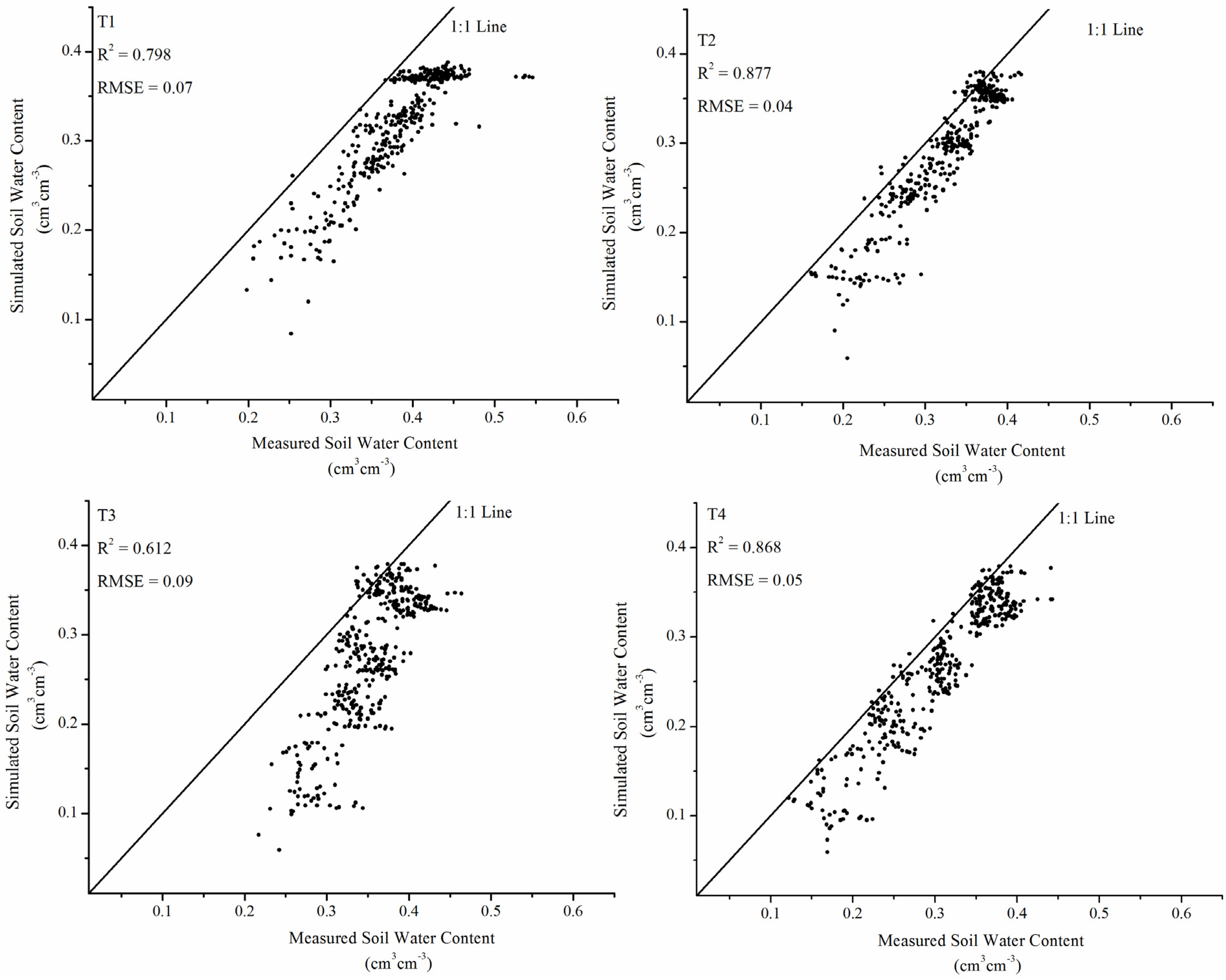
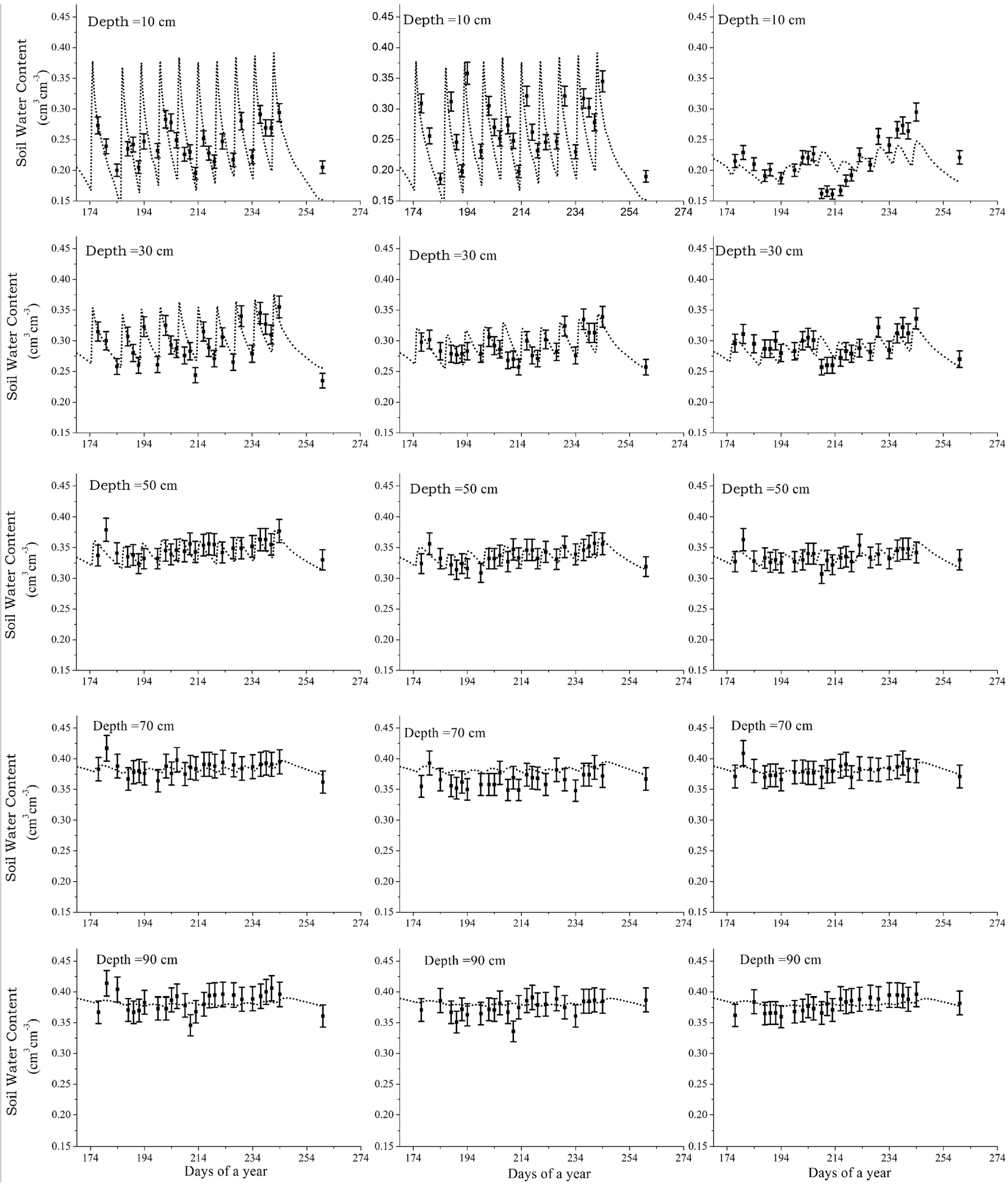
The simulation model (HYDRUS-2D) was calibrated, validated, and applied in a cotton field irrigated by a drip irrigation system under mulch cover. The results suggest that the observed soil water content and the simulated results obtained with HYDRUS-2D are in good agreement. Root water uptake, evaporation, and the radius of the wetting zone decreased as the amount of applied irrigation was reduced (from T1 to T4). Soil water storage and recharge from low soil profiles were increased to compensate for the difference in irrigation. The stored and recharged soil water from low soil layers are highly important water sources, accounting for 3.6%, 15.6%, 27.6%, and 31.1% of water losses for T1, T2, T3, and T4, respectively.
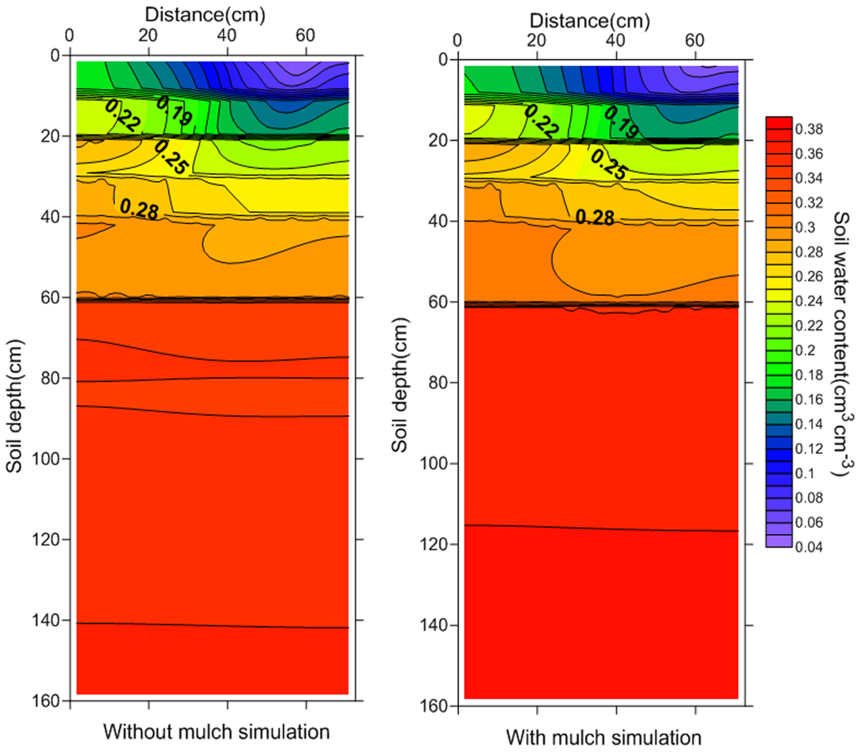
The simulation results revealed that mulch has a minimal effect on soil water distribution patterns. However, mulch is effective for soil water conservation. Evaporation was significantly increased from 3.4 to 25.1 mm after mulch was removed, whereas root water uptake was decreased by 11.2 mm. Drip irrigation under mulch is a widely applied water-saving irrigation technology that can reduce evaporation, improve water use efficiency, and conserve water in extremely arid regions.
In terms of the analysis of the 2D distribution patterns of soil water and water balance components, the HYDRUS-2D model can be applied to assist in the design and development of management practices for drip irrigation systems under mulch cover in arid regions.

Acknowledgments

The study was supported by the Key National Natural Science Foundation (U14003281), (4117095) and National Project (No. 2013BAC10B01) of China and Project SuMaRiO of BMBF (German Federal Ministry of Science and Technology)—Sustainable Management of River Oases along the Tarim River.

Author Contributions

The idea and approach for the study was confirmed by Ming Han and Chengyi Zhao. The majority of the numerical modeling and analysis work was conducted by Ming Han and Gary Feng. Yingyu Yan and Yu Sheng performed the experiments and provided field data. All the authors were involved in preparation of the manuscript.

Conflicts of Interest

The authors declare no conflict of interest.

References

  1. Hou, Z.; Chen, W.; Li, X.; Xiu, L.; Wu, L. Effects of salinity and fertigation practice on cotton yield and 15n recovery. Agric. Water Manag. 2009, 96, 1483–1489. [Google Scholar] [CrossRef]
  2. Ayars, J.; Phene, C.; Hutmacher, R.; Davis, K.; Schoneman, R.; Vail, S.; Mead, R. Subsurface drip irrigation of row crops: A review of 15 years of research at the water management research laboratory. Agric. Water Manag. 1999, 42, 1–27. [Google Scholar] [CrossRef]
  3. Karlberg, L.; Penning de Vries, F.W.T. Exploring potentials and constraints of low-cost drip irrigation with saline water in sub-saharan africa. Phys. Chem. Earth Parts A/B/C 2004, 29, 1035–1042. [Google Scholar] [CrossRef]
  4. Elfving, D. Crop response to trickle irrigation. Hortic. Rev. 1982, 4, 1–48. [Google Scholar]
  5. Shen, X.; Zhang, J.; Liy, Z.; Li, M.; Yang, G.; Sun, J. Effects of different water treatments on yield and water use efficiency of cotton with drip irrigation under film mulch. Agric. Res. Arid Areas 2012, 30, 118–124. [Google Scholar]
  6. Hu, X.T.; Chen, H.; Wang, J.; Meng, X.B.; Chen, F.H. Effects of soil water content on cotton root growth and distribution under mulched drip irrigation. Agric. Sci. China 2009, 8, 709–716. [Google Scholar] [CrossRef]
  7. Zhao, C.; Wang, Y.; Hu, S.; Li, Y. Effects of spatial variability on estimation of evapotranspiration in the continental river basin. J. Arid Environ. 2004, 56, 373–382. [Google Scholar] [CrossRef]
  8. Fang, Y.X.; Zhao, C.Y.; Chuan, Z.Q.; Sheng, Y.; Lin, Q.H. Root distribution characteristics of cotton in different drip irrigation amounts irrigation under mulched. J. Soil Water Conserv. 2007, 21, 96–100. [Google Scholar]
  9. Yan, Y.Y.; Zhao, C.Y.; Sheng, Y.; Li, J.Y.; Peng, D.M.; Li, Z.L.; Feng, S.L. Effects of drip irrigation under mulching on cotton root and shoot biomass and yield. J. Appl. Ecol. 2009, 20, 970–976. [Google Scholar]
  10. Zhao, C.; Yan, Y.; Yimamu, Y.; Li, J.; Zhao, Z.; Wu, L. Effects of soil moisture on cotton root length density and yield under drip irrigation with plastic mulch in aksu oasis farmland. J. Arid Land 2010, 2, 243–249. [Google Scholar]
  11. Zhao, C.Y.; Yan, Y.Y. Distributed characteristics of soil water-salt of cotton field under drip irrigation under mulching in tarim irrigated area. Arid Land Geogr. 2009, 32, 892–898. [Google Scholar]
  12. Zhao, C.Y.; Wang, Y.C.; Li, Z.L.; Li, G.Z. Study on the spatial variability of soil moisture content and salt content in the field scale. Arid Zone Res. 2003, 20, 252–256. [Google Scholar]
  13. Zai, S.M.; Wu, F.; Wen, J.; Han, Q.B. Effect of drip fertigation on soil salinity of cotton field in northwest china. J. Hydraul. Eng. 2011, 42, 1496–1503. [Google Scholar]
  14. Li, F.S.; Lei, X.Y.; Chen, D.C.; Zhou, S.J.; Liu, H.X.; Pan, T. Spatial variability of soil moisture on cotton field under mulched drip irrigation. J. Irrig. Drain. 2010, 28, 10–16. [Google Scholar]
  15. Liu, M.; Yang, J.; Li, X.; Yu, M.; Wang, J. Effects of irrigation water quality and drip tape arrangement on soil salinity, soil moisture distribution, and cotton yield (Gossypium hirsutum L.) under mulched drip irrigation in Xinjiang, China. J. Integr. Agric. 2012, 11, 502–511. [Google Scholar] [CrossRef]
  16. Zhao, C.; Ren, J.; Xue, C.; Lin, E. Study on the relationship between soil selenium and plant selenium uptake. Plant Soil 2005, 277, 197–206. [Google Scholar] [CrossRef]
  17. Zhao, C.; Wang, Y.; Song, Y.; Li, B. Biological drainage characteristics of alakalized desert soils in north-western china. J. Arid Environ. 2004, 56, 1–9. [Google Scholar] [CrossRef]
  18. Yang, Q.; Zuo, H.; Xiao, X.; Wang, S.; Chen, B.; Chen, J. Modelling the effects of plastic mulch on water, heat and CO2 fluxes over cropland in an arid region. J. Hydrol. 2012, 452, 102–118. [Google Scholar] [CrossRef]
  19. Zhang, G.; Hu, X.; Zhang, X.; Li, J. Effect of plastic mulch and winter catch crop on water availability and vegetable yield in a rain-fed vegetable cropping system at mid-yunnan plateau, china. Sci. Hortic. 2013, 164, 333–339. [Google Scholar] [CrossRef]
  20. Hatfield, J.L.; Sauer, T.J.; Prueger, J.H. Managing soils to achieve greater water use efficiency. Agron. J. 2001, 93, 271–280. [Google Scholar] [CrossRef]
  21. Wang, C.; Tian, X.; Li, S. Effects of plastic sheet-mulching on ridge for rainwater-harvesting cultivation on wue and yield of winter wheat. Zhongguo Nongye Kexue 2003, 37, 208–214. [Google Scholar]
  22. Philip, J. Steady infiltration from buried point sources and spherical cavities. Water Resour. Res. 1968, 4, 1039–1047. [Google Scholar] [CrossRef]
  23. Warrick, A. Time-dependent linearized infiltration. I. Point sources. Soil Sci. Soc. Am. J. 1974, 38, 383–386. [Google Scholar] [CrossRef]
  24. Schwartzman, M.; Zur, B. Emitter spacing and geometry of wetted soil volume. J. Irrig. Drain. Eng. 1986, 112, 242–253. [Google Scholar] [CrossRef]
  25. Angelakis, A.N.; Rolston, D.E.; Kadir, T.N.; Scott, V.H. Soil-water distribution under trickle source. J. Irrig. Drain. Eng. 1993, 119, 484–500. [Google Scholar] [CrossRef]
  26. Chu, S.T. Green-ampt analysis of wetting patterns for surface emitters. J. Irrig. Drain. Eng. 1994, 120, 414–421. [Google Scholar] [CrossRef]
  27. Moncef, H.; Hedi, D.; Jelloul, B.; Mohamed, M. Approach for predicting the wetting front depth beneath a surface point source: Theory and numerical aspect. Irrig. Drain. 2002, 51, 347–360. [Google Scholar] [CrossRef]
  28. Cook, F.J.; Thorburn, P.J.; Fitch, P.; Bristow, K.L. Wetup: A software tool to display approximate wetting patterns from drippers. Irrig. Sci. 2003, 22, 129–134. [Google Scholar] [CrossRef]
  29. Kandelous, M.M.; Šimůnek, J. Numerical simulations of water movement in a subsurface drip irrigation system under field and laboratory conditions using hydrus-2d. Agric. Water Manag. 2010, 97, 1070–1076. [Google Scholar] [CrossRef]
  30. Kandelous, M.M.; Šimůnek, J.; van Genuchten, M.T.; Malek, K. Soil water content distributions between two emitters of a subsurface drip irrigation system. Soil Sci. Soc. Am. J. 2011, 75, 488–497. [Google Scholar] [CrossRef]
  31. Ajdary, K.; Singh, D.K.; Singh, A.K.; Khanna, M. Modelling of nitrogen leaching from experimental onion field under drip fertigation. Agric. Water Manag. 2007, 89, 15–28. [Google Scholar] [CrossRef]
  32. Roberts, T.L.; White, S.A.; Warrick, A.W.; Thompson, T.L. Tape depth and germination method influence patterns of salt accumulation with subsurface drip irrigation. Agric. Water Manag. 2008, 95, 669–677. [Google Scholar] [CrossRef]
  33. Ravikumar, V.; Vijayakumar, G.; Šimůnek, J.; Chellamuthu, S.; Santhi, R.; Appavu, K. Evaluation of fertigation scheduling for sugarcane using a vadose zone flow and transport model. Agric. Water Manag. 2011, 98, 1431–1440. [Google Scholar] [CrossRef]
  34. Beggs, R.A.; Hills, D.J.; Tchobanoglous, G.; Hopmans, J.W. Fate of nitrogen for subsurface drip dispersal of effluent from small wastewater systems. J. Contam. Hydrol. 2011, 126, 19–28. [Google Scholar] [CrossRef] [PubMed]
  35. Hanson, B.R.; Šimůnek, J.; Hopmans, J.W. Evaluation of urea-ammonium-nitrate fertigation with drip irrigation using numerical modeling. Agric. Water Manag. 2006, 86, 102–113. [Google Scholar] [CrossRef]
  36. Elmaloglou, S.; Diamantopoulos, E. Simulation of soil water dynamics under subsurface drip irrigation from line sources. Agric. Water Manag. 2009, 96, 1587–1595. [Google Scholar] [CrossRef]
  37. Kandelous, M.M.; Kamai, T.; Vrugt, J.A.; Šimůnek, J.; Hanson, B.; Hopmans, J.W. Evaluation of subsurface drip irrigation design and management parameters for alfalfa. Agric. Water Manag. 2012, 109, 81–93. [Google Scholar] [CrossRef]
  38. Patel, N.; Rajput, T.B.S. Dynamics and modeling of soil water under subsurface drip irrigated onion. Agric. Water Manag. 2008, 95, 1335–1349. [Google Scholar] [CrossRef]
  39. Skaggs, T.; Trout, T.; Šimunek, J.; Shouse, P. Comparison of hydrus-2d simulations of drip irrigation with experimental observations. J. Irrig. Drain. Eng. 2004, 130, 304–310. [Google Scholar] [CrossRef]
  40. Provenzano, G. Using hydrus-2d simulation model to evaluate wetted soil volume in subsurface drip irrigation systems. J. Irrig. Drain. Eng. 2007, 133, 342–349. [Google Scholar] [CrossRef]
  41. Richards, L.A. Capillary conduction of liquids through porous mediums. Physics 1931, 1, 318–333. [Google Scholar] [CrossRef]
  42. Van Genuchten, M.T. A closed-form equation for predicting the hydraulic conductivity of unsaturated soils. Soil Sci. Soc. Am. J. 1980, 44, 892–898. [Google Scholar] [CrossRef]
  43. Šimůnek, J.; van Genuchten, M.T.; Šejna, M. The Hydrus Software Package for Simulating Two- and Three-Dimensional Movement of Water, Heat, and Multiple Solutes in Variably-Saturated Media; PC Progress: Prague, Czech Republic, 2006; p. 241. [Google Scholar]
  44. Allen, R.G.; Pereira, L.S.; Smith, M.; Raes, D.; Wright, J.L. Fao-56 dual crop coefficient method for estimating evaporation from soil and application extensions. J. Irrig. Drain. Eng. 2005, 131, 2–13. [Google Scholar] [CrossRef]
  45. Feddes, R.A.; Kowalik, P.J.; Zaradny, H. Simulation of Field Water Use and Crop Yield; John Wiley & Sons: New York, NY, USA, 1978. [Google Scholar]
  46. Vrugt, J.; Hopmans, J.; Šimunek, J. Calibration of a two-dimensional root water uptake model. Soil Sci. Soc. Am. J. 2001, 65, 1027–1037. [Google Scholar] [CrossRef]
  47. Willmott, C.J. Some comments on the evaluation of model performance. Bull. Am. Meteorol. Soc. 1982, 63, 1309–1313. [Google Scholar] [CrossRef]

