Subgrid Parameterization of the Soil Moisture Storage Capacity for a Distributed Rainfall-Runoff Model

Abstract

Spatial variability plays an important role in nonlinear hydrologic processes. Due to the limitation of computational efficiency and data resolution, subgrid variability is usually assumed to be uniform for most grid-based rainfall-runoff models, which leads to the scale-dependence of model performances. In this paper, the scale effect on the Grid-Xinanjiang model was examined. The bias of the estimation of precipitation, runoff, evapotranspiration and soil moisture at the different grid scales, along with the scale-dependence of the effective parameters, highlights the importance of well representing the subgrid variability. This paper presents a subgrid parameterization method to incorporate the subgrid variability of the soil storage capacity, which is a key variable that controls runoff generation and partitioning in the Grid-Xinanjiang model. In light of the similar spatial pattern and physical basis, the soil storage capacity is correlated with the topographic index, whose spatial distribution can more readily be measured. A beta distribution is introduced to represent the spatial distribution of the soil storage capacity within the grid. The results derived from the Yanduhe Basin show that the proposed subgrid parameterization method can effectively correct the watershed soil storage capacity curve. Compared to the original Grid-Xinanjiang model, the model performances are quite consistent at the different grid scales when the subgrid variability is incorporated. This subgrid parameterization method reduces the recalibration necessity when the Digital Elevation Model (DEM) resolution is changed. Moreover, it improves the potential for the application of the distributed model in the ungauged basin.

1. Introduction

For the last few decades, the development of numerous distributed rainfall-runoff models enables the spatial variations to be represented by a network of grid elements. Advances in geographic information systems (GIS), remote sensing (RS) and computational technology have also offered the potential to build complex distributed hydrologic models and improve the accuracy of hydrologic prediction in time and space [1,2,3].

However, many recent studies have suggested that distributed modelling approaches may not always provide improved simulations at the outlet compared to lumped conceptual models [4]. One of the underlying reasons is that most models do not represent the spatial variability well [5,6]. Limited by the resolution of available data and the computational efficiency, most grid-based distributed models do not take into account the subgrid variability of model input, parameters and model state [7,8,9]. With the assumption of the uniform subgrid, the high frequency information of hydrologic variables and parameters will be lost as the large sampling dimensions act as a filter [10,11].

Because of the nonlinearity of hydrologic processes, model simulations of hydrologic responses are inherently sensitive to the spatial variability of input forcing and watershed characteristics [12]. There is a growing awareness of the sensitivity of small scale variability in hydrologic systems modelling. For example, Wood et al. [13] introduced the concept of the Representative Elementary Area (REA). The REA is defined as a critical threshold at which the implicit continuum assumption can be used without knowledge of the patterns when building the catchment modelling. Arora et al. [14] compared the performances of land surface simulations with and without incorporating the subgrid variability of precipitation intensity and soil moisture. The results indicated that the inclusion of subgrid variability results in significant changes of magnitude, time and frequency of surface runoff generation and partitioning. Ghan et al. [15] assessed the relative influence of the subgrid variability of meteorology, vegetation characteristics, soil properties on surface runoff with a land surface model. They found that neglecting subgrid variability leads to the underestimation of runoff and overestimation of evaporation. Vázquez et al. [16] illustrated the scale-dependence of model effective parameters. They noted that the effective parameters need a recalibration when the grid resolution is changed. The scale-dependence of the model performances and effective parameters makes it a challenge to determine the scale at which the spatial variability can be replaced by grid-averaged characteristics. In order to reduce the necessity of recalibration, it is required to provide a well representation of subgrid variability.

The Grid-Xinanjiang model is an improved version of the Xinanjiang model, which is widely used for flood forecasting in humid and semi-humid area of China [17,18]. The soil storage capacity is a key variable in the Grid-Xinanjiang model, which controls runoff generation and partitioning. Due to the relative short spatial structure, the soil storage capacity is more sensitive to the uniform grid assumption. The bias of estimation of soil storage capacity will introduce the uncertainty of hydrologic simulation, especially for application in the ungauged basin. Therefore, a good representation of subgrid variability of soil storage capacity is necessary for a scale-invariant hydrologic response in the Grid-Xinanjiang model. In this paper, based on the analysis of the model performances of the original Grid-Xinanjiang model at different grid scales, a subgrid parameterization method is presented to account for the subgrid variability of the soil storage capacity.

The rest of paper is organized as follows: in the next section, we provide a description of the study area; a brief description of the Grid-Xinanjiang model and the subgrid parameterization method are presented in the model description section; the following section includes a set of numerical experiments conducted in the Yanduhe Basin to compare the model performance with and without incorporating the subgrid variability; and the final section provides conclusions and perspectives.

2. Study Area

The Yanduhe Basin is located in central China with a catchment area of about 601 km². The Yanduhe River, the main river of the Yanduhe Basin, originating from south of Shennongjia Mountain, flowing into the Yangtze River at 31°14′ N, 110°18′ E, is 60.6 km in length, with a mean slope of 9.5‰. More than 70% of the area is covered by vegetation. The watershed climate is humid, and the average annual precipitation is approximately 1300–1700 mm. Dominated by a monsoon climate, most rainfall occurs during the wet season between April and September.

As shown in Figure 1, the hourly rainfall is monitored at five rainfall gauging stations located in Duizi, Xiagu, Banqiao, Songziyuan and Yanduhe. Hourly streamflow and evaporation data are recorded at the outlet of the watershed. The morphology of the basin is described by the Digital Elevation Model (DEM) with 30 m resolution from the National Aeronautics and Space Administration (NASA). The elevation of the Yanduhe Basin ranges from 130 to 3031 m.

Figure 1. Location and gauging stations of the study area.

Figure 1. Location and gauging stations of the study area.

3. Method

3.1. The Grid-Xinanjiang Model

DEMs are the primary computational elements for rainfall-runoff modeling in the Grid-Xinanjiang model. In each grid cell, canopy interception, direct channel precipitation, evapotranspiration, runoff generation and partitioning are simulated. A simple storage based equation is adopted to calculate the cumulative interception during rainfall events. The precipitation that falls on the channel can be treated as the direct runoff without loss. The evapotranspiration is simulated as a function of moisture content of the vertical soil profile. The soil profile is divided into three layers (upper, lower and deeper layers) in each grid cell to account for the uneven vertical distribution of the soil moisture content. The Grid-Xinanjiang model employs the saturation excess mechanism, and adopts the concept of soil storage capacity to partition the rainfall into runoff and infiltration. Depending on the free water capacity, the runoff is further subdivided into surface runoff, interflow and groundwater runoff.

For the daily simulation, the surface runoff directly routes to the channel as the fast component. The interflow and groundwater runoff represent the slow component that routes to the outlet of the corresponding subcatchment by two linear reservoirs with different lag times. The subcatchments are connected by the channel network. The outflow of each subcatchment is routed to the watershed outlet by the multiple-reach Muskingum method. More details are available in Yao et al. [17] and Liu et al. [19].

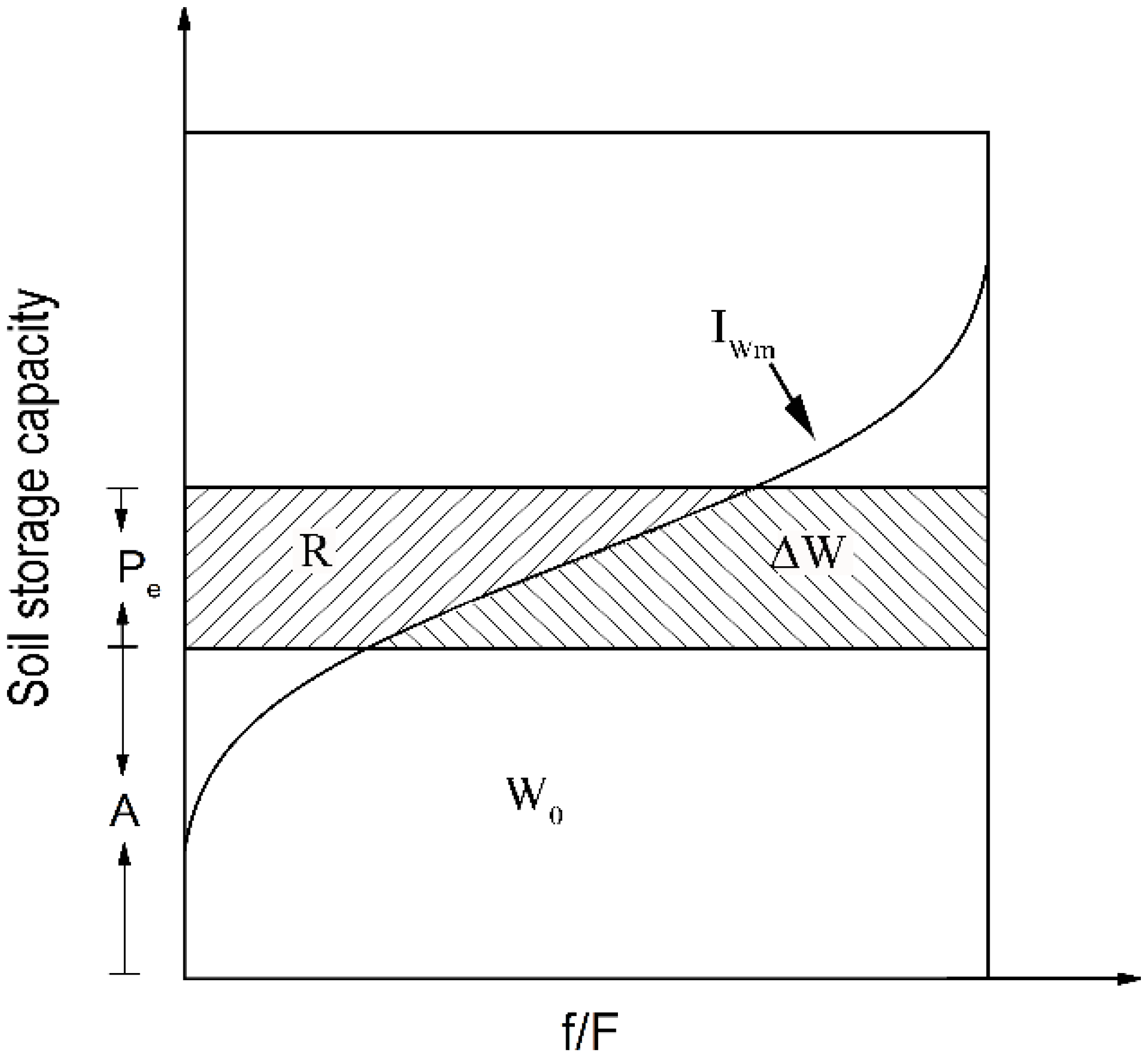
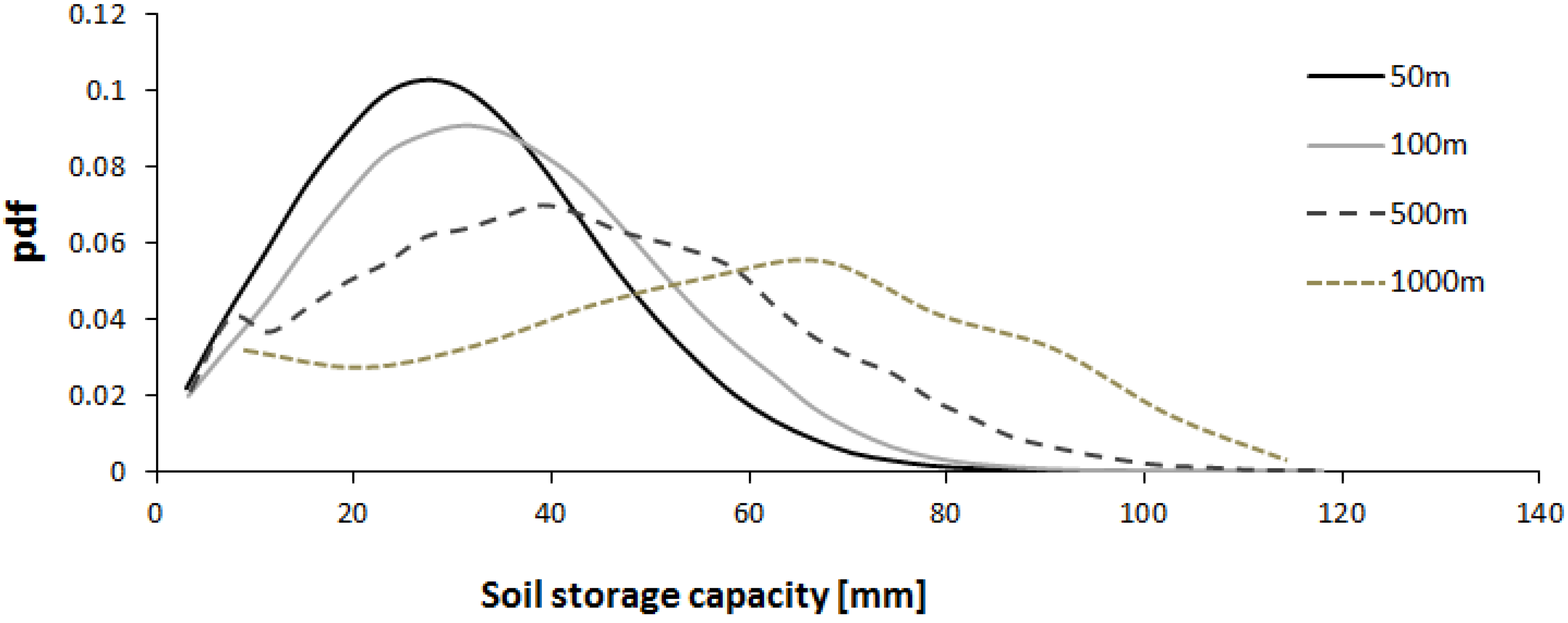
3.2. Subgrid Scale Parameterization of the Soil Storage Capacity

In the original Xinanjiang model, the spatially uneven distribution of the soil storage capacity is depicted by a power function [20]:

$$\frac{f}{F}=1-{\left(1-\frac{WM}{WMM}\right)}^B$$

(1)

where WM is the soil storage capacity, WMM is maximum watershed soil storage capacity, f/F is fraction of basin with the soil storage capacity less than WM, B is exponent of the curve.

A similar method is also adopted in the ARNO [21] and the Variable Infiltration Capacity (VIC) models [22]. The power function provides an analytical solution of runoff generation but lacks definite physical interpretation. Following the work of Williams et al. [23] and Anderson et al. [24], Yao et al. [25] utilized the soil texture and the land cover attributes to estimate the spatial distribution of the soil storage capacity. However, limited by resolution of soil property, the small-scale variability information is not readily available. Therefore, the uniform grid assumption is usually adopted. However, the high frequency information will be smoothed as the uniform grid acts as a filter. Especially for the soil storage capacity, due to the relative short spatial correlation structure, the spatial distribution of the soil storage capacity is more easily affected by the smoothing effect [26,27,28], which may further lead to the scale-dependence of the model performance. Therefore, it is necessary to take into account the subgrid variability of the soil storage capacity in the Grid-Xinanjiang model.

By analyzing the spatial organization of soil moisture and different terrain attributes (slope, mean curvature, topographic index, specific area, etc.), Western et al. [29] demonstrated that the topographic index (TI) can better explain the spatial variability at all scales from 10 m up to the catchment scales. Shi et al. [30] also found a similar spatial pattern between the soil storage capacity and the topographic index. On one hand, topography is an important control of the soil moisture distribution [31,32]. The areas that have large topographic indices usually correspond to the riparian areas, where it is easier to reach saturation because of the relatively small water deficit, and vice versa. On the other hand, the high resolutions of topographic indices are more readily obtained than the soil properties. Shi et al. [30] suggested the topographic index as an auxiliary variable to correlate with the soil storage capacity as following:

$$\frac{WM}{WMM}=\exp \left\{-{\left[\frac{\ln \left(TI-T{I}_{\min }+1\right)}{a}\right]}^b\right\}$$

(2)

where TI_min is the minimum topographic index, a and b are two shape parameters. The topographic index TI is defined as ln(a/tan β), in which a is the cumulative area per unit length of contour line and β is the slope.

As discussed by Pradhan et al. [33], a distinct shift of the value of the topographic index occurs as the DEM resolution becomes coarser. As a function of the topographic index, the soil storage capacity curve also changes correspondingly. Therefore, it is necessary to correct the grid-averaged soil storage capacity. By integrating the soil storage capacity in each grid, we can estimate the total watershed soil storage capacity at each grid scale. The deviation of the total watershed soil storage capacity between the finest grid and other grids can be used to correct the mean value of the soil storage capacity within the grid cell:

$$W{M}_c=WM\frac{WM{M}_t}{WM{M}_c}$$

(3)

where WM_c is the soil storage capacity in each grid after correction, WMM_t is the total watershed soil storage capacity at the finest resolution and WMM_c is the total watershed soil storage capacity at the modelling scale.

As suggested by Li and Avissar [34], here we use a beta distribution to describe the subgrid variability of the soil storage capacity. Compared to the other commonly used probability distribution (gamma, lognormal, etc.), the bounded character of beta distribution is more suitable for the description of soil property. It is defined as following:

$$f(WM)=\frac{\text{Γ}(\text{α}+\text{β})}{\text{Γ}(\text{α})\text{Γ}(\text{β})}W{M}^{\text{α}-1}{(1-WM)}^{\text{β}-1}$$

(4)

where Γ() is the gamma function, and α and β are two shape parameters.

The parameters of the beta distribution can be estimated by the mean and variance values of the soil storage capacity within the grid. We can obtain the mean value of the soil storage capacity of the grid cell by Equations (2) and (3). The variance indicates the fluctuation range of the soil storage capacity within grid which can be derived by spatial aggregation from the finest resolution. Due to the uneven distribution of WM within the grid, part of the effective rainfall (P_e) is partitioned into the runoff (R), and the other part is stored in the soil (ΔW). As shown in Figure 2, the runoff R in a grid can be expressed as:

$$R={\displaystyle {\int }_A^{A+P_e}{P}_e{I}_{WM}}dWM$$

(5)

where A is the soil storage capacity corresponding to the soil content and W₀; I_WM is the cumulative density function of WM.

Figure 2. Schematic representation of runoff generation within a grid.

Figure 2. Schematic representation of runoff generation within a grid.

4. Results and Discussion

4.1. Model Validation

The proposed subgrid parameterization method is validated against the observed data from 1981 to 1986 using a daily time step. The model parameters are calibrated at 30 m resolution with the observations from 1981 to 1984. The rainfall data at five gauging stations is interpolated to each grid using the inverse distance weighting method. Adopting the seeding technology [35], the Yanduhe Basin is subdivided into 58 subcatchments with a threshold of 5 km². We ran a drainage experiment presented by Vivoni [36] to obtain a reasonable spatial distribution of the initial soil moisture. The watershed is assumed to drain from a full saturation status without rainfall and evapotranspiration, until the watershed soil moisture content reaches the condition that we choose. The annual runoff deviation (ARD) and the Nash-Sutcliffe coefficient (NSC) are used as two criteria for the model evaluation. The ARD provides a general sense of the water balance, and the NSC is used to assess the goodness of fit between the simulated and the observed discharge. The ARD and NSC are calculated as follows:

$$ARD=\frac{R_{sim}-R_{obs}}{R_{obs}}\times 100\%$$

(6)

$$NSC=1-\frac{{\displaystyle \sum _n{(Q_{sim}^t-Q_{obs}^t)}^2}}{{\displaystyle \sum _n{(Q_{obs}^t-{\overline{Q}}_{obs})}^2}}$$

(7)

where $R_{sim}$ is the annual simulated runoff; $R_{obs}$ is the annual observed runoff; $Q_{sim}^t$ is the simulated discharge at time step $t$; $Q_{obs}^t$ is the observed discharge at time step $t$; and ${\overline{Q}}_{obs}$ is the mean value of the observed discharge, $n$ is the total number of values in the time period.

The simulated results at the Yanduhe Station are summarized in Table 1. The averaged $ARD$ and $NSC$ are 9% and 0.81 respectively in the calibration periods. In the validation period, the $ARD$ and $NSC$ also reach 10% and 0.76. Figure 3 shows an illustration of the simulated hydrograph against the observed data at the Yanduhe Station from April to October in 1986. The results demonstrate consistency between the simulation and observation. Further analysis is also based on the observed data in 1986.

Table 1. Performance of the Grid-Xinanjiang model for the calibration and validation periods.

Period	Year	ARD (%)	NSC
Calibration	1981	13	0.74
	1982	4	0.90
	1983	7	0.81
	1984	11	0.79
Validation	1985	14	0.65
	1986	6	0.87

Table 1. Performance of the Grid-Xinanjiang model for the calibration and validation periods.

Period	Year	ARD (%)	NSC
Calibration	1981	13	0.74
	1982	4	0.90
	1983	7	0.81
	1984	11	0.79
Validation	1985	14	0.65
	1986	6	0.87

Figure 3. An illustration of the model performance of the Grid-Xinanjiang model with the subgrid parameterization in the Yanduhe Basin in 1986. Red dot, observed discharge; black line, simulated discharge; blue bar, precipitation.

Figure 3. An illustration of the model performance of the Grid-Xinanjiang model with the subgrid parameterization in the Yanduhe Basin in 1986. Red dot, observed discharge; black line, simulated discharge; blue bar, precipitation.

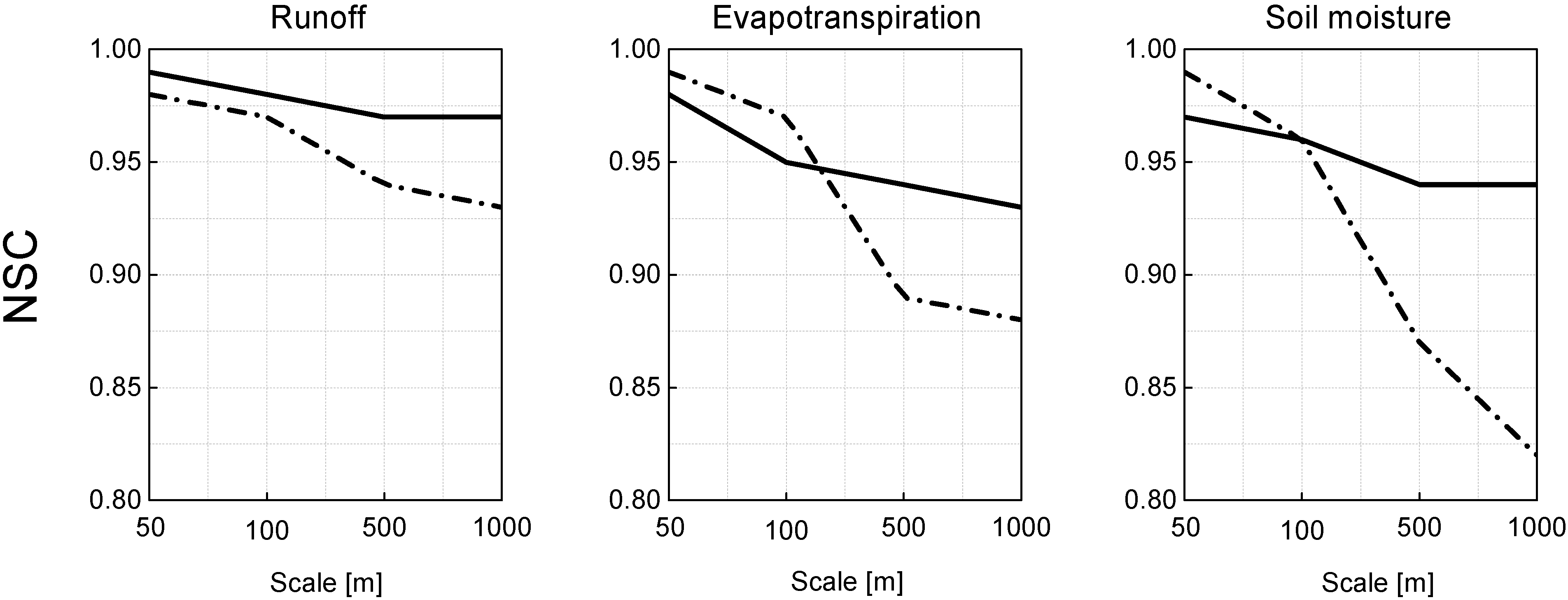
4.2. The Scale-Dependence of the Grid-Xinanjiang Model with a Uniform Grid

The scale-dependence of model performance is the reason that we propose the subgrid parameterization method. Before evaluating the reasonability of the subgrid parameterization, we are also interested in, to what extent, the hydrologic responses of the original Grid-Xinanjiang model depend on the grid scale. Figure 4 depicts the probability density functions of the soil storage capacity from four different grid scales (50 m, 100 m, 500 m and 1000 m) in the Yanduhe Basin. A distinct shift is observed as the grid scale increases. The mean value of the watershed soil storage capacity increases from 30 to 57 mm when the grid scale aggregates from 50 to 1000 m. In addition, the peak of the density function also moves towards a high value. As a key variable in the Grid-Xinanjiang model, the bias indicates that for the coarse grid, more rainfall can be stored in the soil, and the runoff process will be more sensitive to the higher rainfall intensity.

Figure 4. Effect of the grid resolution on the density function of the soil storage capacity.

Figure 4. Effect of the grid resolution on the density function of the soil storage capacity.

The hydrologic responses of the original Grid-Xinanjiang model were evaluated with the observed data from April to October in 1986 in the Yanduhe Basin. Figure 5 shows the processes of the average monthly precipitation, evapotranspiration, runoff and soil moisture at the different resolutions. For comparison, the soil moisture content θ is normalized to the relative soil moisture: θ^* = (θ − θ_r)/(θ_s − θ_r). θ_s and θ_r are the saturation and the residual soil moisture, respectively, the values of which relate to the soil texture [37]. The calibrated parameters at the 30 m resolution are directly adopted without recalibration at each grid scale. As can be seen in Figure 5, all these processes show an obvious scale-dependence. The spatially averaged precipitation reduces with the increasing grid scale. The bias of the precipitation mainly concentrates before March and after August, when the amount of rainfall is relatively low. The maximum margin of the monthly rainfall volume between 50 and 1000 m grids reaches the peak of 8% in September. For the relatively large rainfall volume, such as during June and July, the bias is only approximately 2%. This can be interpreted by the different spatial characteristics of rainfall types. As discussed by Ciach and Krajewski [38], rainfall fields are less variable for higher rainfall intensity. It is obvious that the smoothing effect will be more significant for the storm with higher variability. Compared to the precipitation, the runoff is more sensitive to the change of the grid scale. The bias of the estimation of precipitation, combined with the bias of totally watershed soil storage capacity, results in the inconsistencies of runoff at the different grid scales. For the coarse grid, the precipitation is underestimated. In addition, large soil storage capacity also allows more rainfall stored in the soil, rather than converting into runoff. The averaged bias of runoff between 50 and 1000 m resolution is approximately 28%. The bias of runoff reaches the peak around August. The runoff derived from 50 m is almost three times that from 1000 m. Since more rainfall infiltrates into the soil, the relative soil moisture increases with the grid scale. Therefore, as a function of moisture content of soil profile, the evapotranspiration is correspondingly higher for the coarse grid. The evapotranspiration and the relative soil moisture processes exhibit marked differences between March and August. This is because the evapotranspiration is more intensive during this period. The averaged bias of evapotranspiration and relative soil moisture caused by the spatial aggregation from 50 to 1000 m are 13% and 14%, respectively. Due to the decline of the measured evaporation, only slight differences occur in September and October.

Figure 5. The monthly precipitation, evapotranspiration, runoff and relative soil moisture processes.

Figure 5. The monthly precipitation, evapotranspiration, runoff and relative soil moisture processes.

To evaluate the scale effect on the effective parameters, the model parameters require a recalibration at the different grid scales. To avoid the subjectivity of parameter estimation, automated calibration methods are needed. There has been a great deal of work on the research of automated calibration methods [39,40,41]. In this study, the eleven model parameters are auto-calibrated based on the SCE-UA (Shuffled Complex Evolution method developed at the University of Arizona) algorithm, which has been found to be consistent, effective, and efficient in searching the globally optimum parameters [42,43]. The initial parameters are referred to in Yao et al. [17]. The Nash-Sutcliffe coefficient is used as an objective function. The iteration of SCE-UA algorithm will stop when the objective function cannot improve 0.1% over five iterations or the number of iteration exceeds 10,000. Table 2 lists the value of the effective parameters at four different grid resolutions. It is clear that the model parameters vary with grid scale in varying degrees. The ratio of the potential evapotranspiration to pen evaporation (K), the maximum watershed soil storage capacity (WMM) and the recession constant of the interflow storage (C_i) are relatively sensitive. The ratio of the potential evapotranspiration to pen evaporation decreases from 1.0 to 0.93 when the grid resolution increases from 50 to 1000 m. The maximum watershed soil storage capacity also decrease from 124 to 112. No significant changes were observed for the recession constant of groundwater storage (C_g) and two parameters in the Muskingum routing method (X,V).

Table 2. Model parameters and calibrated values at 4 different grid resolutions.

Parameter	Description	Range	Calibrated value
			50 m	100 m	500 m	1000 m
K	Ratio of potential evapotranspiration to pan evaporation	0–2	1.0	0.98	0.94	0.93
WMM	Maximum watershed soil storage capacity (mm)	60–300	124	118	114	112
α	Shape parameter	0–20	1.1	1.0	0.9	0.9
β	Shape parameter	0–20	1.5	1.5	1.5	1.4
SM	Free water storage capacity (mm)	0–100	12	11	10	10
Ki	Outflow coefficient of free water storage to interflow	0–0.7	0.42	0.40	0.41	0.40
Kg	Outflow coefficient of free water storage to Groundwater	0–0.7	0.28	0.26	0.26	0.25
Ci	Recession constant of interflow storage	0.3–0.8	0.58	0.57	0.54	0.53
Cg	Recession constant of groundwater storage	0.8–0.995	0.85	0.86	0.85	0.84
X	A weight factor of Muskingum method	0.1–0.5	0.33	0.33	0.32	0.32
V	Flow velocity in channel (m/s)	0.5–2	1.3	1.3	1.3	1.3

Table 2. Model parameters and calibrated values at 4 different grid resolutions.

Parameter	Description	Range	Calibrated value
			50 m	100 m	500 m	1000 m
K	Ratio of potential evapotranspiration to pan evaporation	0–2	1.0	0.98	0.94	0.93
WMM	Maximum watershed soil storage capacity (mm)	60–300	124	118	114	112
α	Shape parameter	0–20	1.1	1.0	0.9	0.9
β	Shape parameter	0–20	1.5	1.5	1.5	1.4
SM	Free water storage capacity (mm)	0–100	12	11	10	10
Ki	Outflow coefficient of free water storage to interflow	0–0.7	0.42	0.40	0.41	0.40
Kg	Outflow coefficient of free water storage to Groundwater	0–0.7	0.28	0.26	0.26	0.25
Ci	Recession constant of interflow storage	0.3–0.8	0.58	0.57	0.54	0.53
Cg	Recession constant of groundwater storage	0.8–0.995	0.85	0.86	0.85	0.84
X	A weight factor of Muskingum method	0.1–0.5	0.33	0.33	0.32	0.32
V	Flow velocity in channel (m/s)	0.5–2	1.3	1.3	1.3	1.3

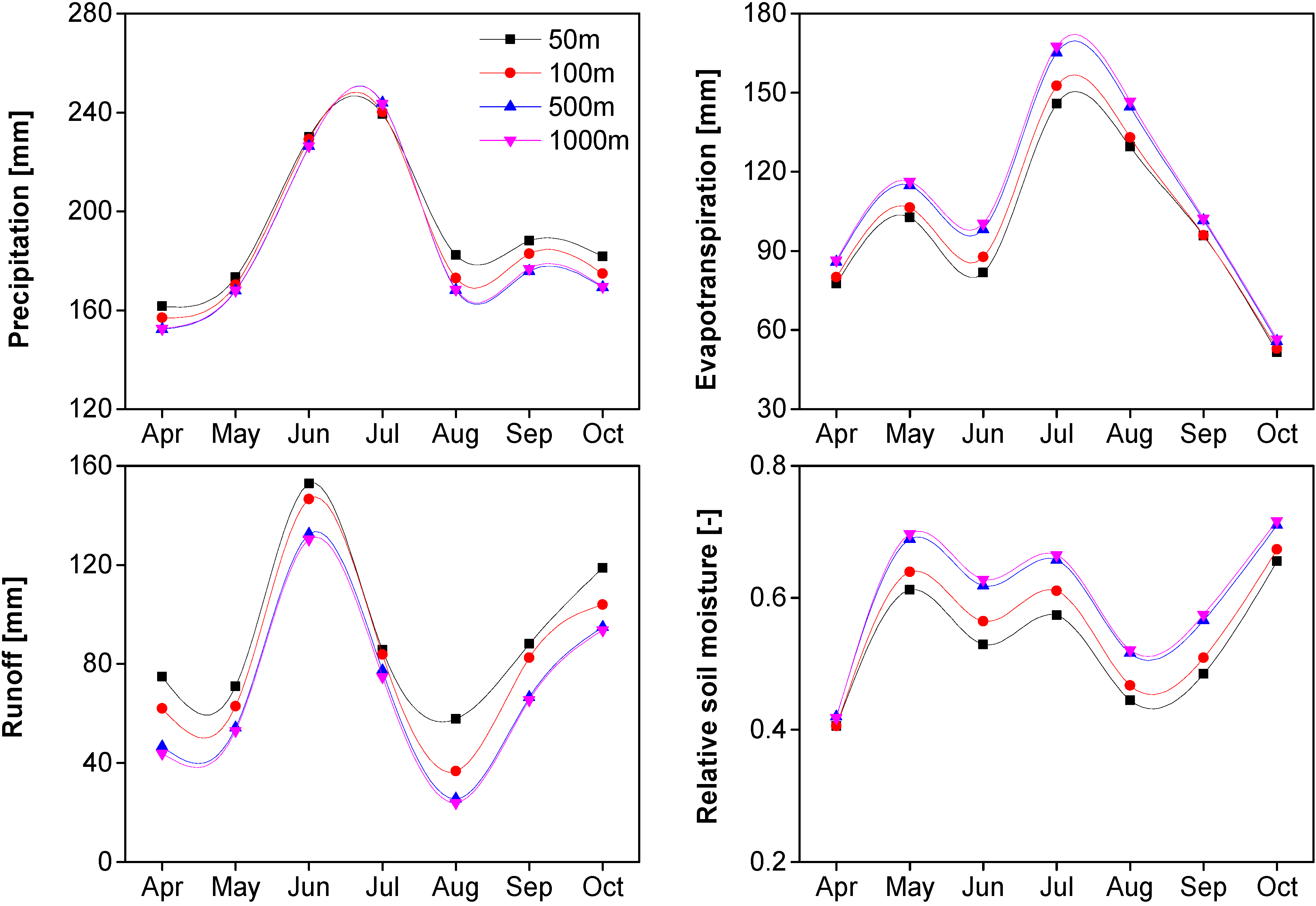
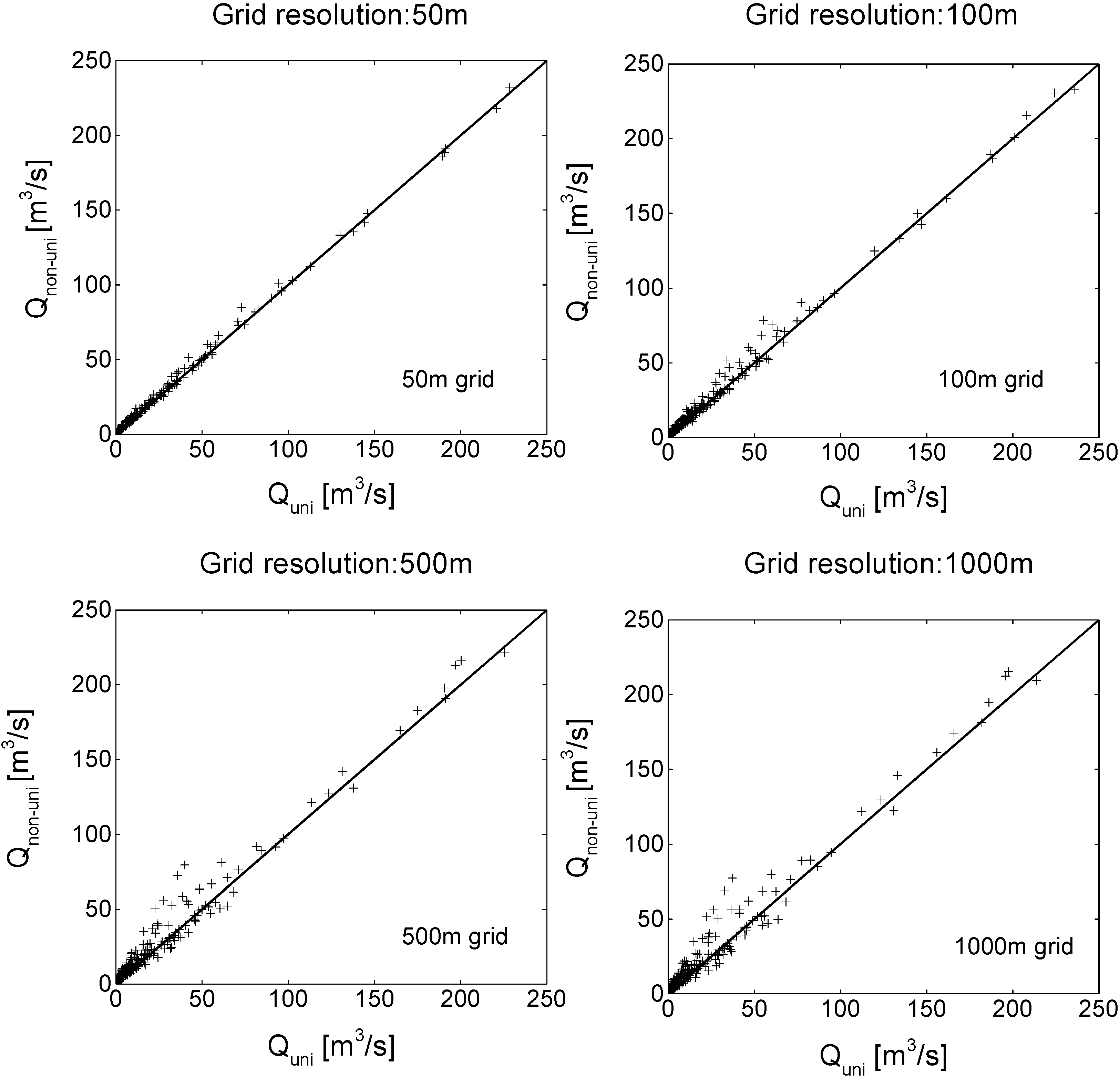
4.3. Evaluation of the Subgrid Parameterization

As discussed above, the bias of the soil storage capacity at the different grid scales is an important reason for the scale-dependence of the model performances and the effective parameters. Therefore, a good representation of soil moisture capacity at the subgrid scale is necessary for a scale-invariant hydrologic response in the Grid-Xinanjiang model. Following the subgrid parameterization described in Section 3, Table 3 compares the annual water budget with and without the subgrid variability. The total annual evapotranspiration (E_p), runoff (R), surface runoff (R_S), interflow (R_I) and groundwater runoff (R_G) at four different resolutions are calculated with the same parameters. As seen in Table 3, with the uniform grid, the annual evapotranspiration increases with the grid scale. The bias of the annual evapotranspiration between 50 and 1000 m resolution can reach 48 mm. The total runoff is significantly underestimated for the coarse grid. The annual total runoff at the 50 m resolution is 852 mm, and 763 mm at the 1000 m resolution. Note that the differences of interflow and groundwater runoff are quite small, and the bias of runoff mainly originates from surface runoff. This is because the runoff is partitioned into different components by the free water capacity, which is relatively small. The impact of the change of the free water capacity on the partitioning of interflow and groundwater runoff is limited. The runoff in excess of the free water capacity converts into surface runoff. Thus, the decrease in the total runoff from fine to coarse grid firstly leads to a change of the surface runoff. However, when the subgrid variability of the soil storage capacity is incorporated, the bias of the annual evapotranspiration between 50 and 1000 m significantly reduces to 3 mm. For the 1000 m resolution, the bias of evapotranspiration with and without the subgrid parameterization are considerably large, accounting for almost 22% of the annual evapotranspiration. For the non-uniform subgrid, the runoff increases by 23 mm and 101 mm for the 50 m and 1000 m resolutions, respectively. Compared to the uniform subgrid, both interflow and groundwater runoff increase marginally after incorporating the subgrid variability, and the differences at different resolutions are almost negligible.

Table 3. Performance of the Grid-Xinanjiang model with and without the subgrid parameterization.

Process	Uniform Subgrid				Non-uniform Subgrid
	50 m	100 m	500 m	1000 m	50 m	100 m	500 m	1000 m
Ep(mm)	472	487	516	520	430	430	427	427
R (mm)	852	819	768	763	876	875	862	864
RS (mm)	244	208	154	147	253	253	242	243
RI (mm)	374	376	378	379	383	383	382	383
RG (mm)	234	235	236	237	239	239	239	239

Table 3. Performance of the Grid-Xinanjiang model with and without the subgrid parameterization.

Process	Uniform Subgrid				Non-uniform Subgrid
	50 m	100 m	500 m	1000 m	50 m	100 m	500 m	1000 m
Ep(mm)	472	487	516	520	430	430	427	427
R (mm)	852	819	768	763	876	875	862	864
RS (mm)	244	208	154	147	253	253	242	243
RI (mm)	374	376	378	379	383	383	382	383
RG (mm)	234	235	236	237	239	239	239	239

In Figure 6, the Nash-Sutcliffe coefficient is used as the criteria to evaluate the model performances of two subgrid schemes at the different grid scale. Because there is no measured data available for the actual evapotranspiration and soil moisture, the simulated results at the 30 m resolution are taken as the true values. In Figure 6, the dash-dot line is obtained from the original Grid-Xinanjiang model, and the solid line represents the model performance after incorporating the subgrid variability. With the uniform grid, the NSC of runoff process ranges between 0.93 and 0.98. The difference is more apparent for evapotranspiration and soil moisture processes. With the same parameters, the NSC of the evapotranspiration and the relative soil moisture decline to 0.88 and 0.82 at 1000 m from 0.98 and 0.97 at 50 m. However, when the subgrid variability is taken into account, the model performances at the different resolutions are quite consistent. The improvement of the model performance is significant, especially at the larger grid scales. The increases of the NSC for the three processes at 1000 m resolution reach 4%, 5% and 12%, respectively. It can be concluded that the subgrid parameterization can partly eliminate the scale-dependence of the model. Not only the total water budget, but also the performance at each time step is quite consistent at each resolution when the subgrid variability is taken into account, but it needs to be pointed out that the proposed subgrid parameterization only depicts the subgrid variability of soil storage capacity, and the variability of precipitation, evapotranspiration or flow routing velocity at the subgrid scale may still cause the inconsistency of model performances at the different grid scales.

Figure 6. Model performances with and without subgrid parameterization. The solid line represents the NSC from the Grid-Xinanjiang model with uniform grid, and the dash-dot line represents the NSC after incorporating the subgrid variability.

Figure 6. Model performances with and without subgrid parameterization. The solid line represents the NSC from the Grid-Xinanjiang model with uniform grid, and the dash-dot line represents the NSC after incorporating the subgrid variability.

To further investigate the effect of subgrid parameterization, Figure 7 plots the simulated discharge at the outlet from the original Grid-Xinanjiang model versus the discharge after incorporating the subgrid variability at 50 m, 100 m, 500 m and 1000 m grid resolutions. It seems that the model tends to underestimate the discharge if the subgrid variability of soil storage capacity is neglected. The gap between the two schemes increases with grid scale. For the 50 m grid resolution, the discharge is closely fit to the 1:1 line. While for the 1000 m resolution, the discharge increases by an average of 6% after incorporating the subgrid variability. The bias of the discharge with and without subgrid variability can be as high as 40 m³/s. The large bias between the two schemes mainly occurs when the discharge is less than 100 m³/s. Even for small discharge, the gap is also evident. However, no significant change is observed for large discharge. It is because, for the saturation excess mechanism employed by the Grid-Xinanjiang model, large discharge is usually associated with relatively high soil content and intense rainfall. Once the watershed is fully saturated, all of the effective rainfall will directly convert into the runoff without loss. In this case, the effect of the spatial variability on runoff will no longer exist. It demonstrates that the subgrid variability is more necessary for the relatively dry period. This conclusion not only works for the Grid-Xinanjiang model, but also for the other saturation excess dominated hydrologic model.

Figure 7. Discharge from the original Grid-Xinanjiang model (Q_uni) versus runoff after incorporating the subgrid variability (Q_non-uni).

Figure 7. Discharge from the original Grid-Xinanjiang model (Q_uni) versus runoff after incorporating the subgrid variability (Q_non-uni).

5. Conclusions

Spatial variability is known to increase with scale. With the assumption of a uniform grid, the spatial averaging operation leads to the scale-dependence of model performance. In this study, we take the Grid-Xinanjiang model as an example to investigate the effect of subgrid variability on the hydrologic response. The processes of precipitation, runoff, evapotranspiration and soil moisture at four different grid scales (50 m, 100 m, 500 m and 1000 m) are compared. The calibrated parameters based on 30 m resolution are used for each simulation without recalibration. The results derived from the Yanduhe Basin show that the model performances vary with grid scales. As a key variable in the Grid-Xinanjiang model, the total watershed soil storage capacity increases from 30 to 57 mm when the grid resolution spatially aggregates from 50 to 1000 m. Depending on the different rainfall structure, the precipitation is underestimated for coarse grid. The bias of precipitation process and watershed soil storage capacity leads to the inconsistency of the hydrologic responses across scales. Calibrated by the SCE-UA method against the observed data, the model effective parameters also vary with grid scale in varying degrees.

Therefore, for a scale-invariant hydrologic response, the subgrid variability is required to be taken into account. In light of the sensitivity of the Grid-Xinanjiang model to the soil storage capacity, this study presents a subgrid parameterization method to incorporate the subgrid variability of the soil storage capacity. The topographic index is adopted as an auxiliary variable to correlate the soil storage capacity. On one hand, the topographic index and the soil storage capacity have similar spatial distributions and physical basis. On the other hand, the high resolution topographic index is more readily obtained than the soil property information. A beta distribution is introduced to represent the spatial distribution of the soil storage capacity within grid cell. Compared to the original Grid-Xinanjiang model, the simulated runoff, evapotranspiration and soil moisture processes are quite consistent at different grid scales when the subgrid variability is incorporated. The inclusion of the subgrid variability results in a significant increase of runoff and a decrease of evapotranspiration. For the annual water budget, the differences of runoff and evapotranspiration with and without incorporating the subgrid variability can reach 101 mm and 93 mm respectively at the 1000 m resolution. Due to the saturation excess mechanism employed by the Grid-Xinanjiang model, the correction of hydrologic responses resulting from subgrid parameterization is more obvious for relatively small rainfall event or dry conditions. The subgrid parameterization method benefits to reduce the necessity of recalibration when DEM resolution is changed, but it also needs to be noted that the proposed parameterization method only partly eliminates the scale-dependence of the runoff generation. Further research deserves more attention on the scale effect on flow routing.

References

1. Paniconi, C.; Wood, E.F. A detailed model for simulation of catchment scale subsurface hydrologic processes. Water Resour. Res. 1993, 29, 1601–1620. [Google Scholar] [CrossRef]
2. Abbott, M.B.; Bathurst, J.C.; Cunge, J.A.; O’Connell, P.E.; Rasmussen, J. An introduction to the European Hydrological System—Systeme Hydrologique Europeen, “SHE”, 1: History and philosophy of a physically-based, distributed modelling system. J. Hydrol. 1986, 87, 45–59. [Google Scholar] [CrossRef]
3. Blöschl, G.; Reszler, C.; Komma, J. A spatially distributed flash flood forecasting model. Environ. Model. Softw. 2008, 23, 464–478. [Google Scholar] [CrossRef]
4. Reed, S.; Koren, V.; Smith, M.; Zhang, Z.; Moreda, F.; Seo, D.-J.; Dmip Participants. Overall distributed model intercomparison project results. J. Hydrol. 2004, 298, 27–60. [Google Scholar] [CrossRef]
5. Carpenter, T.M.; Georgakakos, K.P. Impacts of parametric and radar rainfall uncertainty on the ensemble streamflow simulations of a distributed hydrologic model. J. Hydrol. 2004, 298, 202–221. [Google Scholar] [CrossRef]
6. Smith, M.B.; Koren, V.I.; Zhang, Z.; Reed, S.M.; Pan, J.-J.; Moreda, F. Runoff response to spatial variability in precipitation: An analysis of observed data. J. Hydrol. 2004, 298, 267–286. [Google Scholar] [CrossRef]
7. Ciarapica, L.; Todini, E. TOPKAPI: A model for the representation of the rainfall-runoff process at different scales. Hydrol. Process. 2002, 16, 207–229. [Google Scholar] [CrossRef]
8. Beven, K.; Freer, J. A dynamic TOPMODEL. Hydrol. Process. 2001, 15, 1993–2011. [Google Scholar] [CrossRef]
9. Dehotin, J.; Braud, I. Which spatial discretization for distributed hydrological models? Proposition of a methodology and illustration for medium to large-scale catchments. Hydrol. Earth Syst. Sci. 2008, 12, 769–796. [Google Scholar] [CrossRef]
10. Band, L.E.; Moore, I.D. Scale: Landscape attributes and geographical information systems. Hydrol. Process. 1995, 9, 401–422. [Google Scholar] [CrossRef]
11. Kavvas, M.L. On the coarse-graining of hydrologic processes with increasing scales. J. Hydrol. 1999, 217, 191–202. [Google Scholar] [CrossRef]
12. Beven, K. How far can we go in distributed hydrological modelling? Hydrol. Earth Syst. Sci. 1999, 5, 1–12. [Google Scholar] [CrossRef]
13. Wood, E.F.; Sivapalan, M.; Beven, K.; Band, L. Effects of spatial variability and scale with implications to hydrologic modeling. J. Hydrol. 1988, 102, 29–47. [Google Scholar] [CrossRef]
14. Arora, V.K.; Chiew, F.H.S.; Grayson, R.B. Effect of sub-grid-scale variability of soil moisture and precipitation intensity on surface runoff and streamflow. J. Geophys. Res. 2001, 106, 17073–17091. [Google Scholar] [CrossRef]
15. Ghan, S.J.; Liljegren, J.C.; Shaw, W.J.; Hubbe, J.H.; Doran, J.C. Influence of Subgrid Variability on Surface Hydrology. J. Clim. 1997, 10, 3157–3166. [Google Scholar] [CrossRef]
16. Vázquez, R.F.; Feyen, L.; Feyen, J.; Refsgaard, J.C. Effect of grid size on effective parameters and model performance of the MIKE-SHE code. Hydrol. Process. 2002, 16, 355–372. [Google Scholar] [CrossRef]
17. Yao, C.; Li, Z.; Bao, H.; Yu, Z. Application of a Developed Grid-Xinanjiang Model to Chinese Watersheds for Flood Forecasting Purpose. J. Hydrol. Eng. 2009, 14, 923–934. [Google Scholar] [CrossRef]
18. Zhao, R.; Liu, X. The Xinanjiang model. In Computer Models of Watershed Hydrology; Singh, V., Ed.; Water Resources Publications: Littleton, CO, USA, 1995; pp. 215–232. [Google Scholar]
19. Liu, J.; Chen, X.; Zhang, J.; Flury, M. Coupling the Xinanjiang model to a kinematic flow model based on digital drainage networks for flood forecasting. Hydrol. Process. 2009, 23, 1337–1348. [Google Scholar] [CrossRef]
20. Zhao, R. The Xinanjiang model applied in China. J. Hydrol. 1992, 135, 371–381. [Google Scholar]
21. Todini, E. The ARNO rainfall—Runoff model. J. Hydrol. 1996, 175, 339–382. [Google Scholar] [CrossRef]
22. Wood, E.F.; Lettenmaier, D.P.; Zartarian, V.G. A land-surface hydrology parameterization with subgrid variability for general circulation models. J. Geophys. Res. 1992, 97, 2717–2728. [Google Scholar] [CrossRef]
23. Williams, J.; Ouyang, Y.; Chen, J.-S.; Ravi, V.; Jewett, D.S.B.D.G. Estimation of Infiltration Rate in Vadose Zone: Application of Selected Mathematical Models; Office of Research and Development, United States Environmental Protection Agency: Washington, DC, USA, 1998. [Google Scholar]
24. Anderson, R.M.; Koren, V.I.; Reed, S.M. Using SSURGO data to improve Sacramento Model a priori parameter estimates. J. Hydrol. 2006, 320, 103–116. [Google Scholar] [CrossRef]
25. Yao, C.; Li, Z.; Yu, Z.; Zhang, K. A priori parameter estimates for a distributed, grid-based Xinanjiang model using geographically based information. J. Hydrol. 2012, 468–469; 47–62. [Google Scholar] [CrossRef]
26. Famiglietti, J.S.; Ryu, D.; Berg, A.A.; Rodell, M.; Jackson, T.J. Field observations of soil moisture variability across scales. Water Resour. Res. 2008. [Google Scholar] [CrossRef]
27. Western, A.W.; Blöschl, G.; Grayson, R.B. Geostatistical characterisation of soil moisture patterns in the Tarrawarra catchment. J. Hydrol. 1998, 205, 20–37. [Google Scholar] [CrossRef]
28. Western, A.W.; Zhou, S.-L.; Grayson, R.B.; McMahon, T.A.; Blöschl, G.; Wilson, D.J. Spatial correlation of soil moisture in small catchments and its relationship to dominant spatial hydrological processes. J. Hydrol. 2004, 286, 113–134. [Google Scholar] [CrossRef]
29. Western, A.W.; Grayson, R.B.; Blöschl, G.; Willgoose, G.R.; McMahon, T.A. Observed spatial organization of soil moisture and its relation to terrain indices. Water Resour. Res. 1999, 35, 797–810. [Google Scholar] [CrossRef]
30. Shi, P.; Rui, X.; Qu, S.; Chen, X. Development and application of a grid-based distributed hydrological model. Dv. In Water Sci. 2008, 19, 662–670. [Google Scholar]
31. Woods, R.A.; Sivapalan, M.; Robinson, J.S. Modeling the spatial variability of subsurface runoff using a topographic index. Water Resour. Res. 1997, 33, 1061–1073. [Google Scholar] [CrossRef]
32. Hjerdt, K.N.; McDonnell, J.J.; Seibert, J.; Rodhe, A. A new topographic index to quantify downslope controls on local drainage. Water Resour. Res. 2004, 40. [Google Scholar] [CrossRef]
33. Pradhan, N.R.; Tachikawa, Y.; Takara, K. A downscaling method of topographic index distribution for matching the scales of model application and parameter identification. Hydrol. Process. 2006, 20, 1385–1405. [Google Scholar] [CrossRef]
34. Li, B.; Avissar, R. The Impact of Spatial Variability of Land-Surface Characteristics on Land-Surface Heat Fluxes. J. Clim. 1994, 7, 527–537. [Google Scholar] [CrossRef]
35. Jenson, S.K.; Domingue, J.O. Extracting topographic structure from digital elevation data for geographic information system analysis. Photogramm. Eng. Remote Sens. 1988, 54, 1593–1600. [Google Scholar]
36. Vivoni, E.R.; Entekhabi, D.; Bras, R.L.; Ivanov, V.Y. Controls on runoff generation and scale-dependence in a distributed hydrologic model. Hydrol. Earth Syst. Sci. Discuss. 2007, 11, 1683–1701. [Google Scholar]
37. Rawls, W.; Brakensiek, D.; Miller, N. Green-ampt Infiltration Parameters from Soils Data. J. Hydraul. Eng. 1983, 109, 62–70. [Google Scholar] [CrossRef]
38. Ciach, G.J.; Krajewski, W.F. Analysis and modeling of spatial correlation structure in small-scale rainfall in Central Oklahoma. Adv. Water Resour. 2006, 29, 1450–1463. [Google Scholar] [CrossRef]
39. Chen, W.; Chau, K. Intelligent manipulation and calibration of parameters for hydrological models. Int. J. Environ. Pollut. 2006, 28, 432–447. [Google Scholar] [CrossRef]
40. Gupta, V.; Sorooshian, S. Calibration of conceptual hydrologic models: Past, present and future. In Trends in Hydrology. Research Trends; Council of Scientific Research Integration: Trivandrum, India, 1994; pp. 329–346. [Google Scholar]
41. Taormina, R.; Chau, K.-W. Neural network river forecasting with multi-objective fully informed particle swarm optimization. J. Hydroinform. 2015, 17, 99–113. [Google Scholar] [CrossRef]
42. Duan, Q.; Sorooshian, S.; Gupta, V.K. Optimal use of the SCE-UA global optimization method for calibrating watershed models. J. Hydrol. 1994, 158, 265–284. [Google Scholar] [CrossRef]
43. Duan, Q.Y.; Gupta, V.K.; Sorooshian, S. Shuffled complex evolution approach for effective and efficient global minimization. J. Optim. Theory Appl. 1993, 76, 501–521. [Google Scholar] [CrossRef]