
Daily Runoff Forecasting Model Based on ANN and Data Preprocessing Techniques


Abstract
:1. Introduction
2. Data-Driven Models
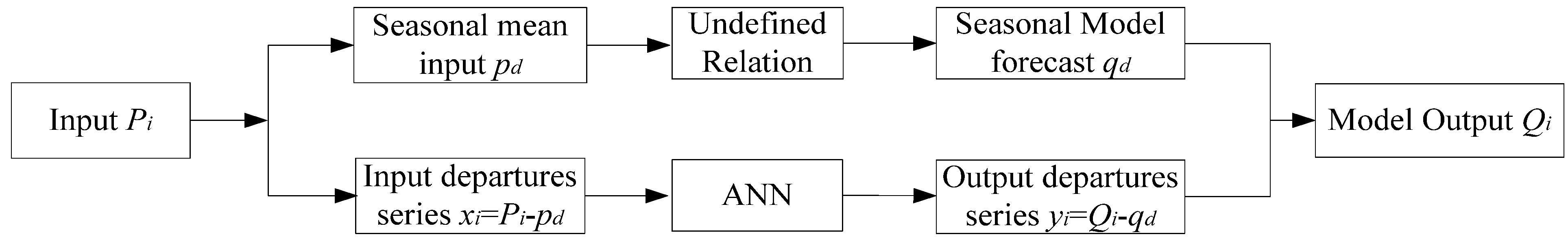
2.1. NLPM-ANN Model

2.2. Singular Spectrum Analysis
2.3. Artificial Neural Network
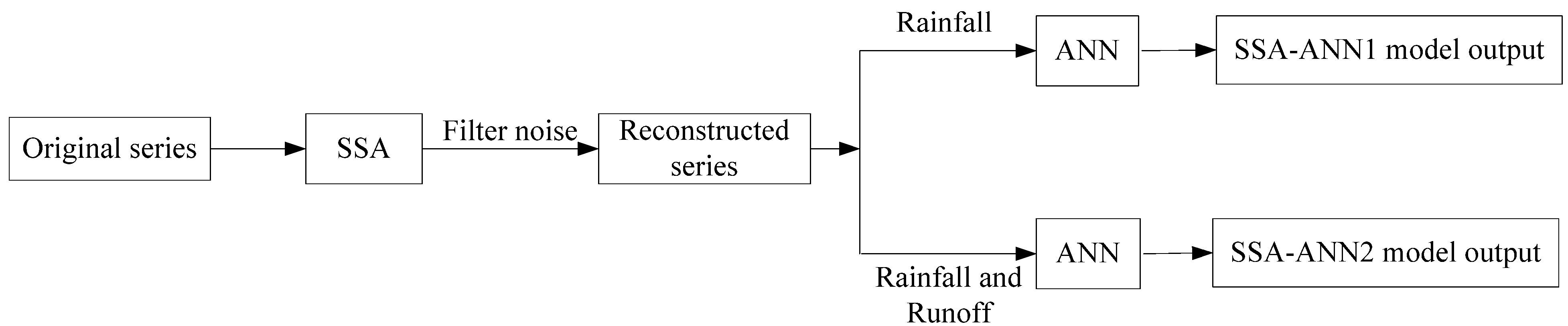
2.4. Proposed SSA-ANN Models

2.5. Evaluation of Model Performances
- (1)
- Determination coefficient (or Nash-Sutcliffe criterion) (R2)
- (2)
- Water balance coefficient (WB)
3. Comparative Study
3.1. Data

| Watershed and Datasets | Statistical Parameters | Data Period | |||||
|---|---|---|---|---|---|---|---|
| μ | Sx | Xmax | Xmin | ||||
| Jiahe area: 5578 km2 | rainfall (mm) | whole data | 2.3 | 5.9 | 71.4 | 0 | January 1980–December 1990 |
| training data | 2.3 | 6.0 | 68.9 | 0 | |||
| cross-validation data | 2.3 | 6.2 | 71.4 | 0 | |||
| testing data | 2.1 | 5.3 | 44.2 | 0 | |||
| runoff (m3) | whole data | 58.7 | 125.1 | 2620 | 6.5 | ||
| training data | 61.9 | 141.6 | 2620 | 6.5 | |||
| cross-validation data | 55.3 | 99.6 | 1220 | 7.9 | |||
| testing data | 50.7 | 76.4 | 1080 | 10.1 | |||
| Laoguanhe area: 4217 km2 | rainfall (mm) | whole data | 2.2 | 6.4 | 69.4 | 0 | January 1980–December 1990 |
| training data | 2.3 | 6.8 | 69.2 | 0 | |||
| cross-validation data | 2.0 | 5.8 | 56.0 | 0 | |||
| testing data | 2.0 | 5.7 | 69.4 | 0 | |||
| runoff (m3) | whole data | 27.1 | 73.6 | 1460 | 0.1 | ||
| training data | 33.5 | 84.1 | 1460 | 0.4 | |||
| cross-validation data | 16.8 | 50.6 | 586 | 0.1 | |||
| testing data | 14.8 | 46.1 | 793 | 0.2 | |||
| Baohe area: 3415 km2 | rainfall (mm) | whole data | 2.5 | 6.9 | 80.6 | 0 | January 1980–December 1990 |
| training data | 2.5 | 7.1 | 80.6 | 0 | |||
| cross-validation data | 2.2 | 6.0 | 51.3 | 0 | |||
| testing data | 2.6 | 6.8 | 80.5 | 0 | |||
| runoff (m3) | whole data | 46.5 | 129.4 | 4020 | 0 | ||
| training data | 49.7 | 150.7 | 4020 | 1.2 | |||
| cross-validation data | 31.4 | 54.8 | 523 | 3.8 | |||
| testing data | 50.3 | 96.8 | 2010 | 0.0 | |||
| Mumahe area: 1224 km2 | rainfall (mm) | whole data | 3.2 | 8.8 | 132.8 | 0 | January 1980–December 1990 |
| training data | 3.2 | 8.6 | 132.8 | 0 | |||
| cross-validation data | 3.3 | 9.3 | 98.6 | 0 | |||
| testing data | 2.9 | 9.1 | 94.4 | 0 | |||
| runoff (m3) | whole data | 39.3 | 80.3 | 1270 | 1.2 | ||
| training data | 41.0 | 80.8 | 1270 | 1.2 | |||
| cross-validation data | 40.6 | 82.1 | 796 | 4.6 | |||
| testing data | 32.1 | 76.4 | 990 | 2 | |||
| Nianyushan area: 924 km2 | rainfall (mm) | whole data | 3.8 | 11.6 | 269.5 | 0 | January 1975–December 1999 |
| training data | 3.9 | 12.2 | 269.5 | 0 | |||
| cross-validation data | 3.3 | 9.3 | 102.5 | 0 | |||
| testing data | 3.7 | 10.8 | 144.7 | 0 | |||
| runoff (m3) | whole data | 18.5 | 62.1 | 2095 | 0 | ||
| training data | 19.8 | 68.3 | 2095 | 0 | |||
| cross-validation data | 13.5 | 33.2 | 508 | 0 | |||
| testing data | 17.6 | 55.9 | 822 | 0 | |||
| Gaoguan area: 303 km2 | rainfall (mm) | whole data | 4.2 | 12.5 | 179.1 | 0 | January 1984–December 1999 |
| training data | 4.4 | 12.8 | 179.1 | 0 | |||
| cross-validation data | 3.5 | 11.3 | 143.8 | 0 | |||
| testing data | 4.2 | 12.7 | 116.0 | 0 | |||
| runoff (m3) | whole data | 5.8 | 15.1 | 246 | 0 | ||
| training data | 5.7 | 14.2 | 237 | 0 | |||
| cross-validation data | 5.1 | 13.5 | 246 | 0 | |||
| testing data | 7.7 | 20.5 | 214 | 0 | |||
| Shimen area: 271.25 km2 | rainfall (mm) | whole data | 3.8 | 11.4 | 141.3 | 0 | January 1989–December 1999 |
| training data | 3.5 | 10.1 | 114.9 | 0 | |||
| cross-validation data | 5.1 | 15.1 | 141.3 | 0 | |||
| testing data | 3.8 | 11.8 | 116.8 | 0 | |||
| runoff (m3) | whole data | 4.9 | 15.2 | 296 | 0 | ||
| training data | 3.7 | 9.9 | 150 | 0 | |||
| cross-validation data | 8.7 | 25.1 | 296 | 0 | |||
| testing data | 5.5 | 17.9 | 172 | 0 | |||
| Tiantang area: 220 km2 | rainfall (mm) | whole data | 3.7 | 12.1 | 193.4 | 0 | January 1973–December 1984 |
| training data | 3.6 | 11.6 | 175.0 | 0 | |||
| cross-validation data | 3.7 | 11.4 | 151.7 | 0 | |||
| testing data | 4.2 | 14.7 | 193.4 | 0 | |||
| runoff (m3) | whole data | 6.1 | 18.4 | 535 | 0 | ||
| training data | 5.6 | 16.5 | 400 | 0 | |||
| cross-validation data | 5.6 | 16.5 | 378 | 0.3 | |||
| testing data | 8.2 | 25.6 | 535 | 0.3 | |||
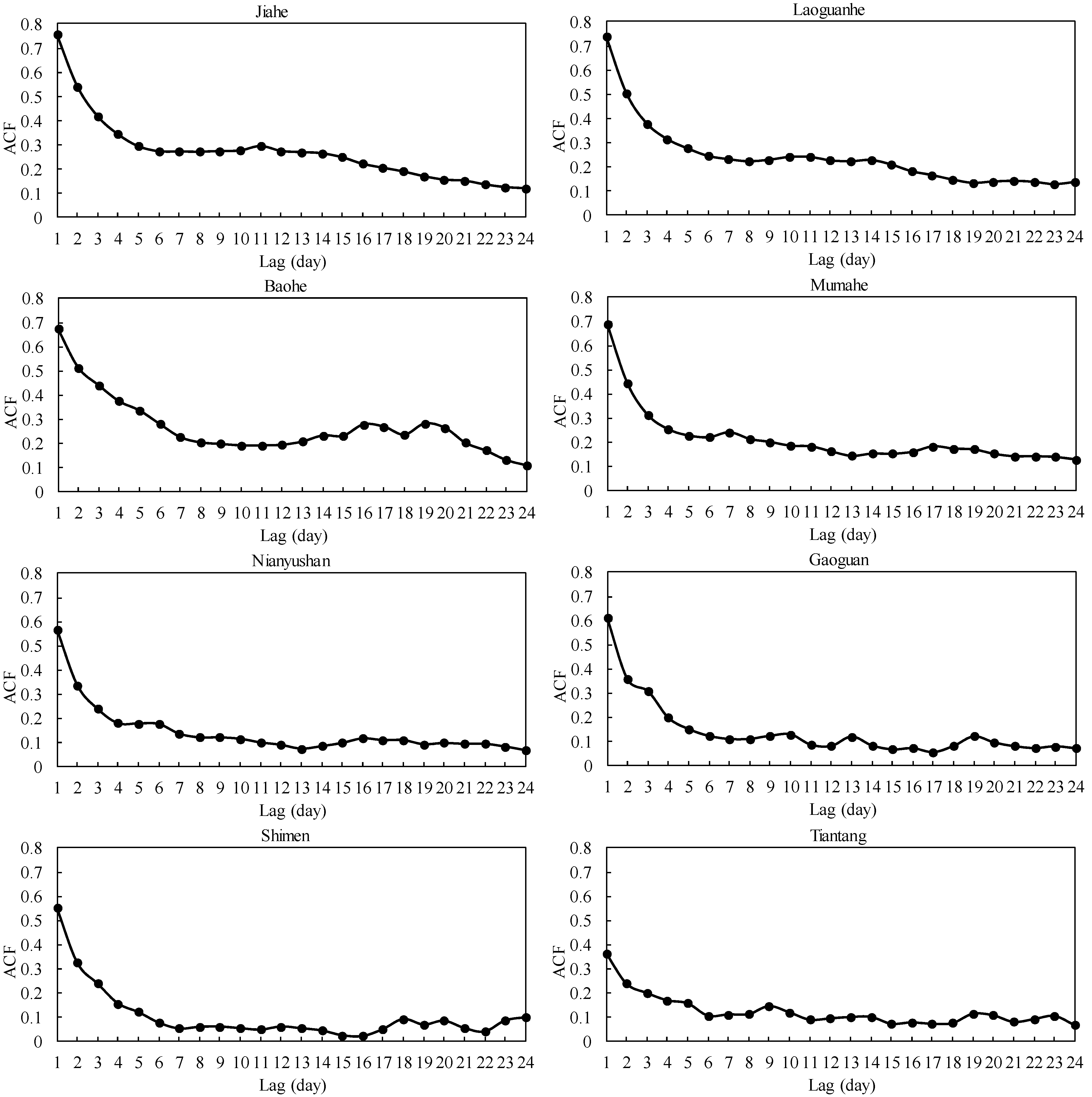
3.2. Determination of Model Inputs

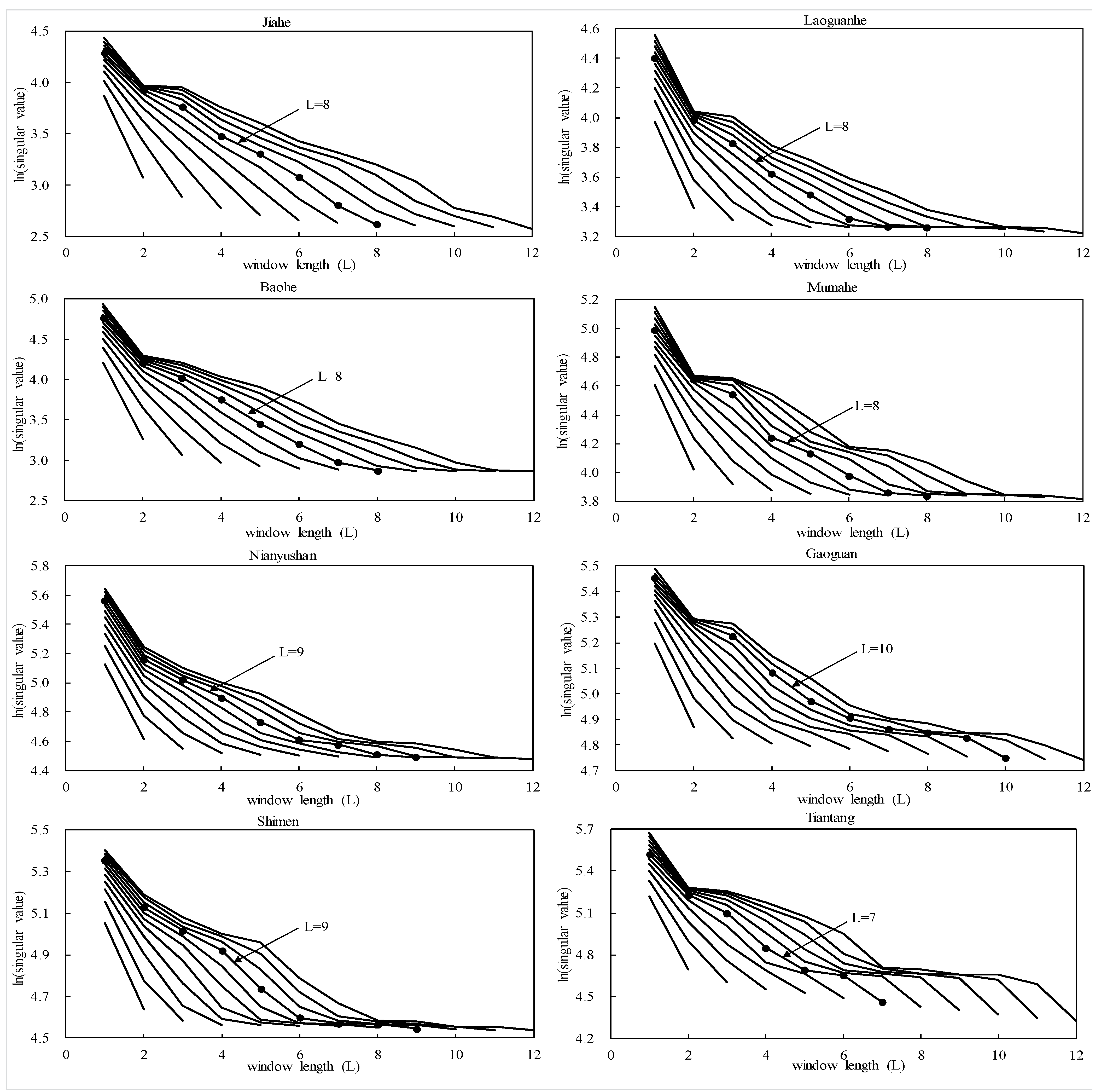
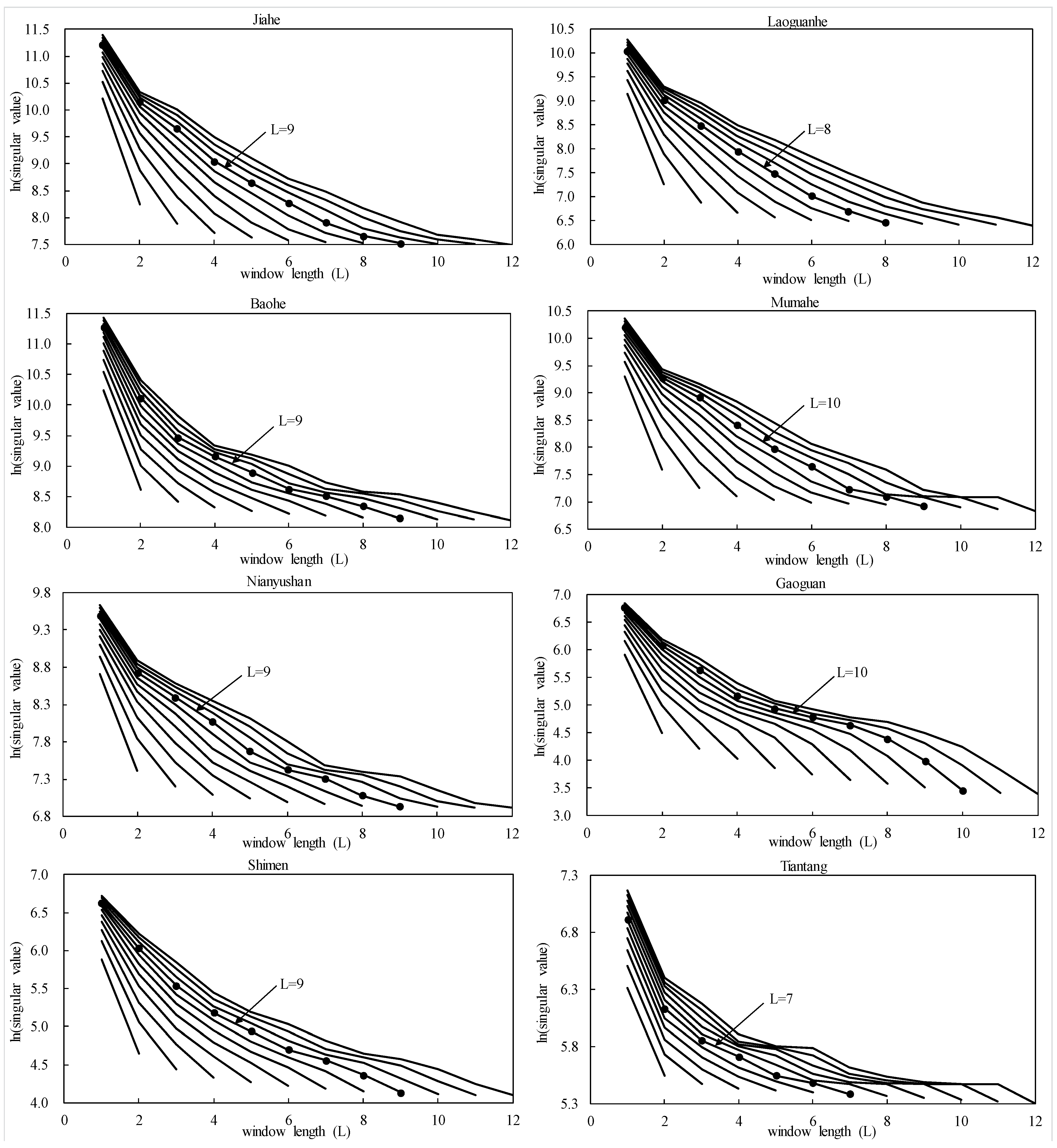
3.3. Data Preprocessing


| Watershed | Decomposed Components | L | p | ||||||||||
|---|---|---|---|---|---|---|---|---|---|---|---|---|---|
| 1 | 2 | 3 | 4 | 5 | 6 | 7 | 8 | 9 | 10 | ||||
| Jiahe | rainfall | −0.26 | −0.27 | −0.19 | −0.05 | 0.13 | 0.36 | 0.50 | 0.55 | – | – | 8 | 4 |
| runoff | −0.14 | −0.15 | −0.11 | −0.05 | 0.05 | 0.18 | 0.39 | 0.55 | 0.77 | – | 9 | 5 | |
| Laoguanhe | rainfall | −0.36 | −0.33 | −0.24 | −0.06 | 0.12 | 0.33 | 0.47 | 0.53 | – | – | 8 | 4 |
| runoff | −0.15 | −0.15 | −0.10 | 0.00 | 0.14 | 0.35 | 0.55 | 0.77 | – | – | 8 | 4 | |
| Baohe | rainfall | −0.26 | −0.26 | −0.18 | −0.04 | 0.14 | 0.35 | 0.50 | 0.60 | – | – | 8 | 4 |
| runoff | −0.18 | −0.20 | −0.16 | −0.08 | 0.04 | 0.16 | 0.33 | 0.54 | 0.76 | – | 9 | 5 | |
| Mumahe | rainfall | −0.34 | −0.32 | −0.22 | −0.06 | 0.13 | 0.34 | 0.47 | 0.52 | – | – | 8 | 4 |
| runoff | −0.15 | −0.18 | −0.14 | −0.09 | −0.01 | 0.11 | 0.25 | 0.41 | 0.56 | 0.71 | 10 | 5 | |
| Nianyushan | rainfall | −0.33 | −0.33 | −0.26 | −0.13 | 0.02 | 0.19 | 0.35 | 0.47 | 0.51 | – | 9 | 5 |
| runoff | −0.22 | −0.22 | −0.16 | −0.03 | 0.15 | 0.34 | 0.54 | 0.68 | – | – | 8 | 4 | |
| Gaoguan | rainfall | −0.32 | −0.37 | −0.30 | −0.18 | −0.07 | 0.09 | 0.23 | 0.37 | 0.46 | 0.43 | 10 | 5 |
| runoff | −0.14 | −0.19 | −0.17 | −0.12 | −0.03 | 0.09 | 0.23 | 0.42 | 0.58 | 0.67 | 10 | 5 | |
| Shimen | rainfall | −0.34 | −0.34 | −0.32 | −0.28 | 0.01 | 0.19 | 0.35 | 0.47 | 0.48 | – | 9 | 5 |
| runoff | −0.21 | −0.23 | −0.18 | −0.09 | 0.04 | 0.19 | 0.39 | 0.58 | 0.66 | – | 9 | 5 | |
| Tiantang | rainfall | −0.32 | −0.34 | −0.19 | 0.03 | 0.28 | 0.46 | 0.53 | – | – | – | 7 | 4 |
| runoff | −0.31 | −0.31 | −0.16 | 0.03 | 0.25 | 0.46 | 0.62 | – | – | – | 7 | 4 | |
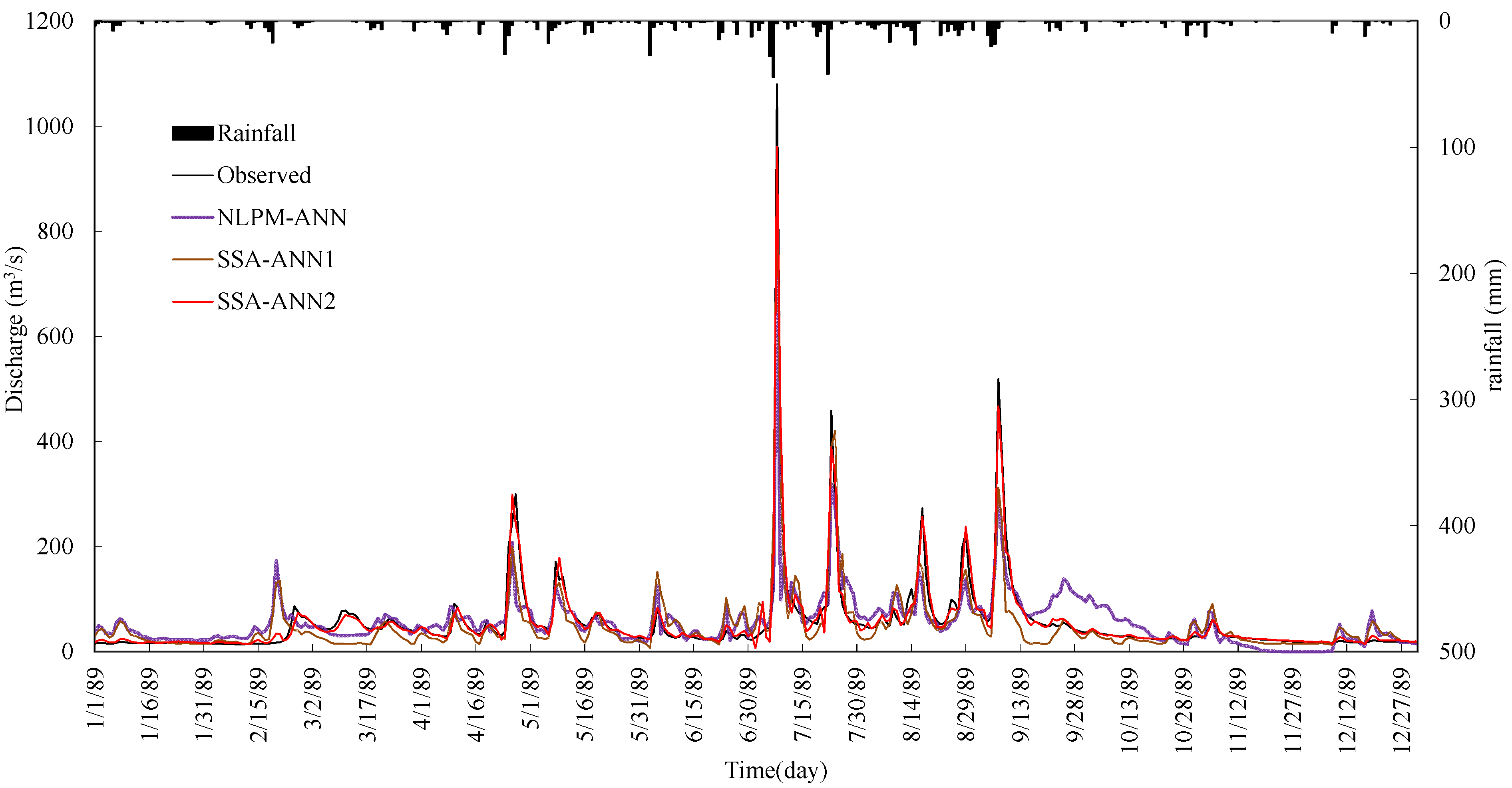
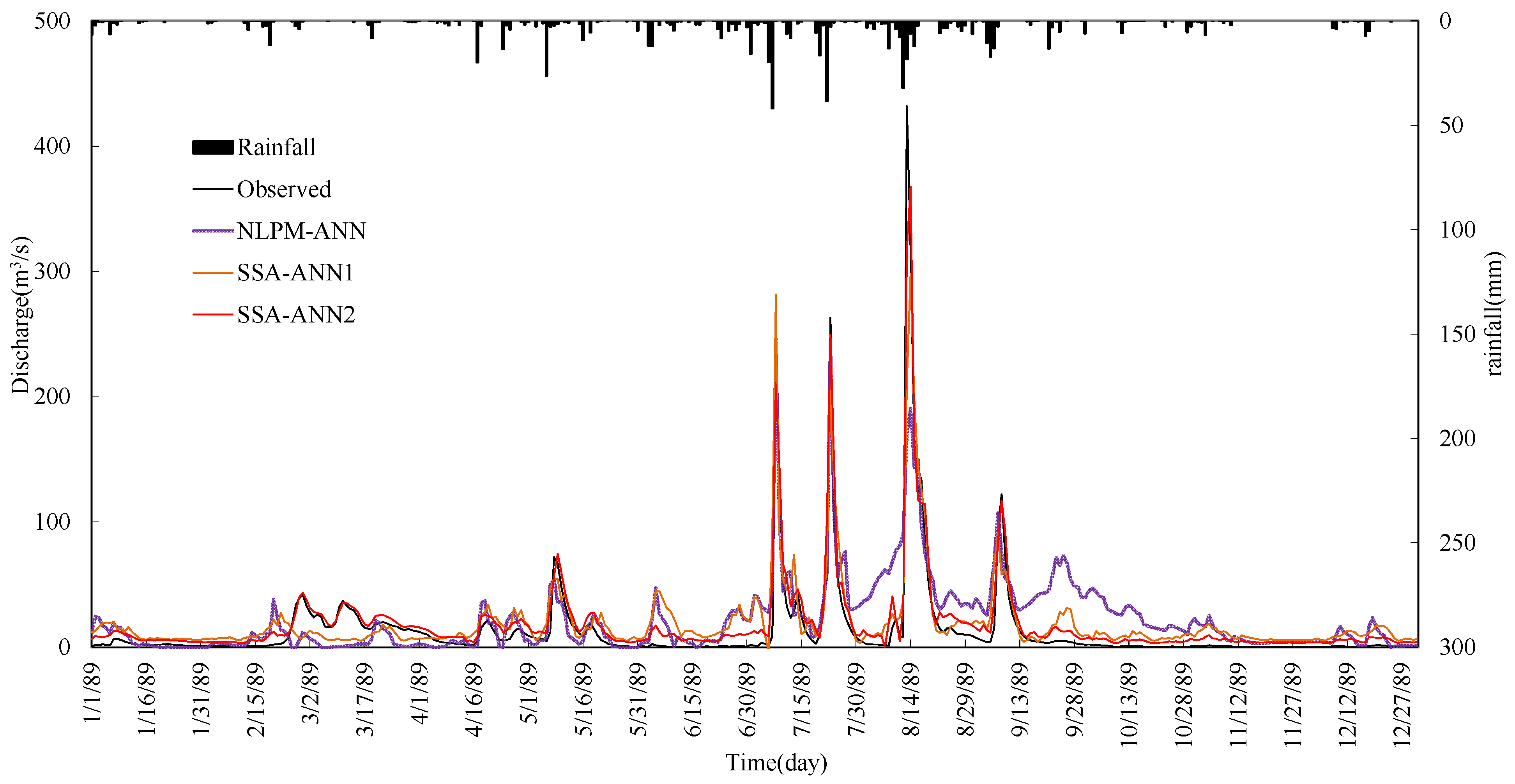
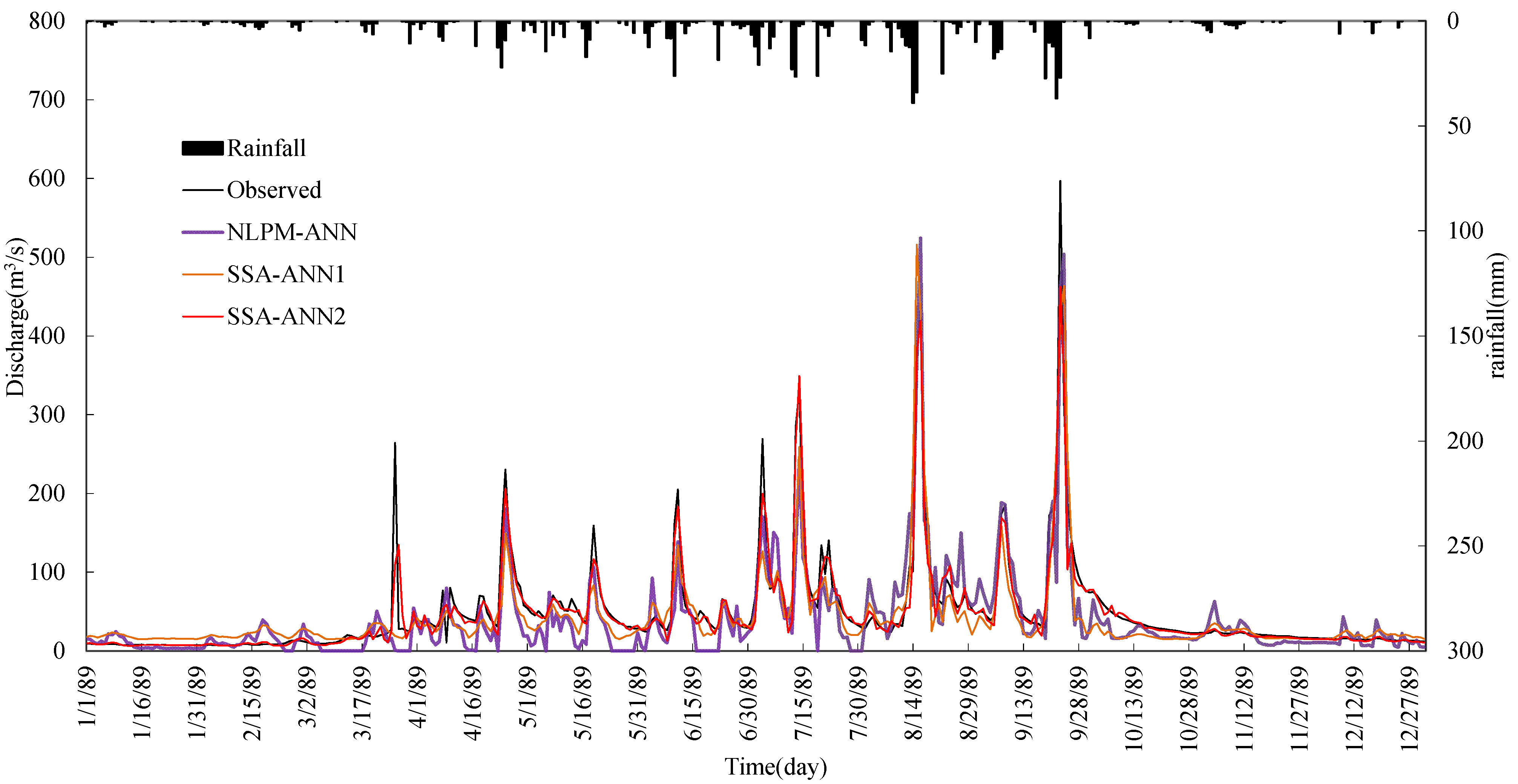
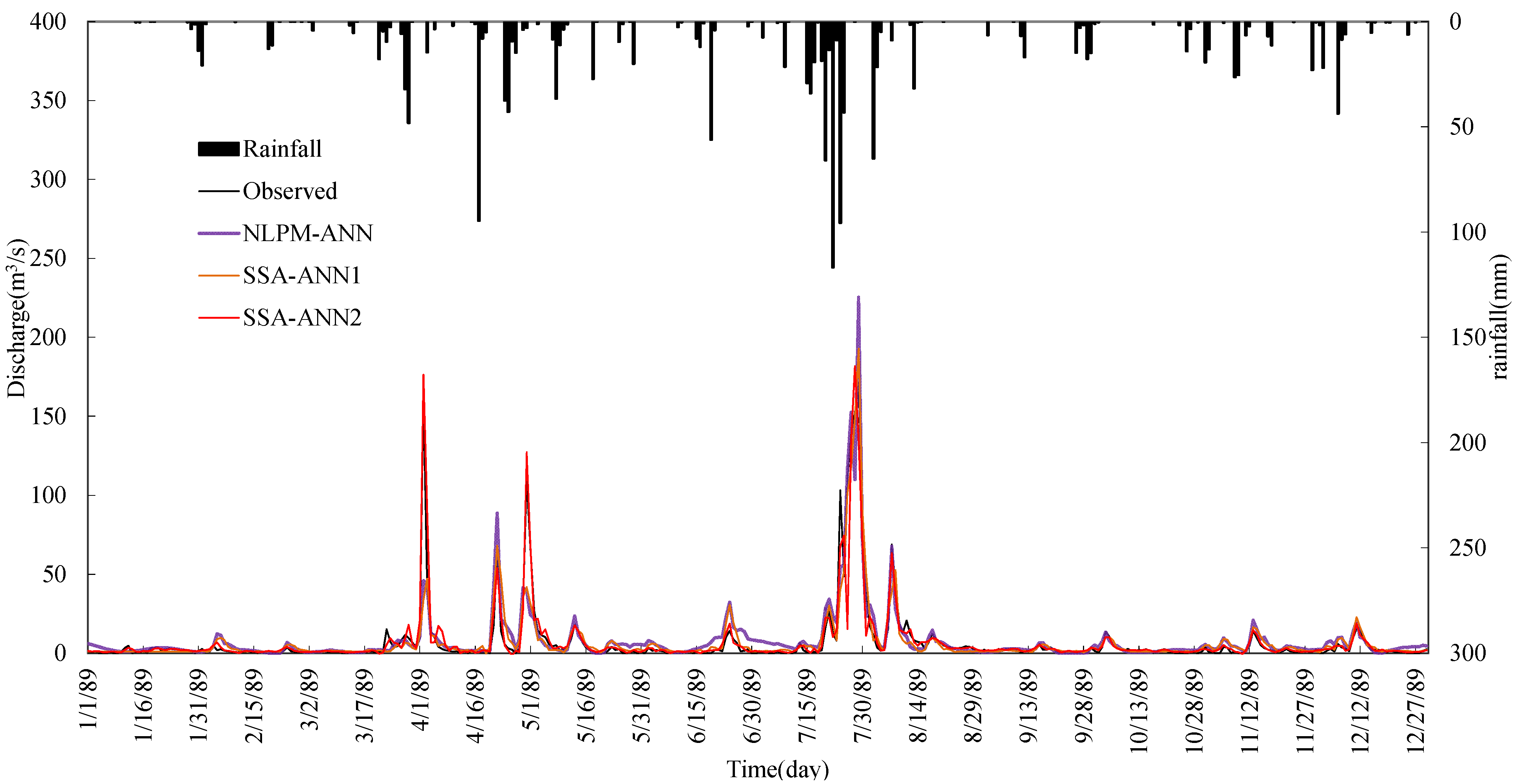
4. Results Analysis
| Watershed | ANN | NLPM-ANN | SSA-ANN1 | SSA-ANN2 | |||||
|---|---|---|---|---|---|---|---|---|---|
| R2 (%) | WB | R2 (%) | WB | R2 (%) | WB | R2 (%) | WB | ||
| Jiahe | calibration | 68.19 | 1.023 | 85.46 | 1.015` | 80.97 | 0.982 | 96.09 | 1.013 |
| testing | 61.48 | 0.866 | 61.31 | 1.119 | 74.91 | 0.975 | 92.40 | 1.013 | |
| Laoguanhe | calibration | 69.72 | 1.048 | 85.66 | 1.042 | 82.29 | 0.972 | 96.31 | 1.186 |
| testing | 60.42 | 1.058 | 68.25 | 1.412 | 78.44 | 1.464 | 93.20 | 1.407 | |
| Baohe | calibration | 64.75 | 0.975 | 70.93 | 1.039 | 88.50 | 1.029 | 94.01 | 1.006 |
| testing | 68.62 | 0.667 | 69.38 | 0.893 | 74.03 | 0.927 | 94.31 | 0.956 | |
| Mumahe | calibration | 80.64 | 0.950 | 90.18 | 1.050 | 87.86 | 0.976 | 95.08 | 1.019 |
| testing | 80.17 | 0.913 | 85.6 | 1.410 | 92.41 | 1.108 | 94.71 | 1.053 | |
| Nianyushan | calibration | 75.8 | 0.941 | 83.44 | 1.084 | 84.89 | 0.910 | 85.86 | 1.020 |
| testing | 82.38 | 0.803 | 85.39 | 1.329 | 88.30 | 0.939 | 88.39 | 1.077 | |
| Gaoguan | calibration | 66.16 | 1.035 | 77.6 | 1.045 | 80.17 | 1.002 | 93.24 | 1.005 |
| testing | 76.38 | 0.957 | 77.97 | 0.894 | 80.43 | 0.840 | 89.85 | 0.962 | |
| Shimen | calibration | 65.03 | 0.848 | 64.85 | 1.068 | 73.85 | 1.141 | 94.53 | 1.084 |
| testing | 72 | 0.772 | 75.72 | 1.281 | 76.90 | 1.089 | 87.99 | 1.055 | |
| Tiantang | calibration | 65.47 | 0.985 | 73.06 | 1.049 | 78.08 | 0.960 | 88.66 | 1.131 |
| testing | 59.79 | 0.895 | 81.96 | 0.956 | 79.54 | 1.015 | 91.32 | 1.043 | |
| Mean | calibration | 69.47 | 0.976 | 78.41 | 1.046 | 82.08 | 1.00 | 92.97 | 1.06 |
| testing | 70.16 | 0.879 | 75.86 | 1.155 | 80.62 | 1.04 | 91.52 | 1.07 | |


5. Summary and Conclusions
- (1)
- The performance of the ANN model can be improved by data preprocessing techniques. SSA is more effective and it can improve the learning and training ability of the ANN type model significantly. Results also show that the impact of noise in hydrological time series on model performance is bigger than the seasonal hydrological behavior.
- (2)
- Comparing the SSA-ANN1 model with the NLPM-ANN model, the mean values of R2 and WB for the SSA-ANN1 model are 82.08% and 80.62%, and 1.0 and 1.04, during calibration and testing periods, respectively, which are much better than that of the NLPM-ANN model.
- (3)
- The SSA-ANN2 model performs best for daily runoff forecasting for all selected watersheds. The effective way for increasing daily runoff forecasting accuracy is to preprocess data series by SSA and select both previous related rainfall and runoff as predictive factors.
- (4)
- There are some limitations in this study. The method to select the contributing components relies on liner correlation analysis, which disregards the existence of nonlinearity in the hydrologic process. The sensitivities and uncertainties of model parameters are not analyzed. All of these will be the focus in our future research.
Acknowledgment
Author Contributions
Conflicts of Interest
References
- Baratti, R.; Cannas, B.; Fanni, A.; Pintus, M.; Sechi, G.M.; Toreno, N. River flow forecast for reservoir management through neural networks. Neurocomputing 2003, 55, 421–437. [Google Scholar] [CrossRef]
- Chang, F.J.; Chen, Y.C. A counterpropagation fuzzy-neural network modeling approach to real time streamflow prediction. J. Hydrol. 2001, 245, 153–164. [Google Scholar] [CrossRef]
- Nayak, P.C.; Sudheer, K.P.; Ramasastri, K.S. Fuzzy computing based rainfall–runoff model for real time flood forecasting. Hydrol. Process. 2005, 19, 955–968. [Google Scholar] [CrossRef]
- French, M.N.; Krajewski, W.F.; Cuykendall, R.R. Rainfall forecasting in space and time using a neural network. J. Hydrol. 1992, 137, 1–31. [Google Scholar] [CrossRef]
- Hsu, K.L.; Gupta, H.V.; Sorooshian, S. Artificial neural network modeling of the rainfall–runoff process. Water Resour. Res. 1995, 31, 2517–2530. [Google Scholar] [CrossRef]
- Sivakumar, B.; Liong, S.Y.; Liaw, C.Y. Evidence of chaotic behavior in Singapore rainfall. J. Am. Water Resour. Assoc. 1998, 34, 301–310. [Google Scholar] [CrossRef]
- Whigam, P.A.; Crapper, P.F. Modelling rainfall–runoff relationships using genetic programming. Math. Comput. Model. 2001, 33, 707–721. [Google Scholar] [CrossRef]
- Liong, S.Y.; Sivapragasm, C. Hood stage forecasting with SVM. J. Am. Water Resour. Assoc. 2002, 38, 173–186. [Google Scholar] [CrossRef]
- Govindaraju, R.S. Artificial neural networks in hydrology. I: Preliminary concepts. J. Hydrol. Eng. 2000, 5, 115–123. [Google Scholar]
- Govindaraju, R.S. Artificial neural networks in hydrology. II: Hydrological applications. J. Hydrol. Eng. 2000, 5, 124–137. [Google Scholar]
- Maier, H.R.; Dandy, G.C. Neural networks for the prediction and forecasting of water resources variables: A review of modelling issues and applications. Environ. Modell. Softw. 2000, 15, 101–124. [Google Scholar] [CrossRef]
- Dawson, C.W.; Wilby, R.L. Hydrological modeling using artificial neural networks. Progr. Phys. Geogr. 2001, 25, 80–108. [Google Scholar] [CrossRef]
- Sudheer, K.P.; Gosain, A.K.; Ramasastri, K.S. A data-driven algorithm for constructing artificial neural network rainfall-runoff models. Hydrol. Process. 2002, 16, 1325–1330. [Google Scholar] [CrossRef]
- Xiong, L.H.; O’Connor, K.M.; Guo, S.L. Comparison of three updating schemes using Artificial Neural Network in flow forecasting. Hydrol. Earth Syst. Sci. 2004, 8, 247–255. [Google Scholar] [CrossRef]
- Kumar, A.R.S.; Sudheer, K.P.; Jain, S.K.; Agarwal, P.K. Rainfall-runoff modelling using artificial neural networks: Comparison of network types. Hydrol. Process. 2005, 19, 1277–1291. [Google Scholar] [CrossRef]
- Pang, B.; Guo, S.L.; Xiong, L.H.; Li, C.Q. A nonlinear perturbation model based on artificial neural network. J. Hydrol. 2007, 333, 504–516. [Google Scholar] [CrossRef]
- Rezaeian, Z.M.; Amin, S.; Khalili, D.; Singh, V.P. Daily outflow prediction by multilayer perceptron with logistic sigmoid and tangent sigmoid activation functions. Water Resour. Manag. 2010, 24, 2673–2688. [Google Scholar] [CrossRef]
- Rezaeian, Z.M.; Stein, A.; Tabari, H.; Abghari, H.; Jalalkamali, N.; Hosseinipour, E.Z.; Singh, V.P. Assessment of a conceptual hydrological model and artificial neural networks for daily out-flows forecasting. Int. J. Environ. Sci. Technol. 2013, 10, 1181–1192. [Google Scholar] [CrossRef]
- Shamseldin, A.Y. Artificial neural network model for river flow forecasting in a developing country. J. Hydroinform. 2010, 12, 22–35. [Google Scholar] [CrossRef]
- Wu, J.S.; Han, J.; Annambhotla, S.; Bryant, S. Artificial neural networks for forecasting watershed runoff and stream flows. J. Hydrol. Eng. 2005, 10, 216–222. [Google Scholar] [CrossRef]
- Taormina, R.; Chau, K. Neural network river forecasting with multi-objective fully informed particle swarm optimization. J. Hydroinform. 2015, 17, 99–113. [Google Scholar] [CrossRef]
- Wu, C.L.; Chau, K.W.; Li, Y.S. Methods to improve neural network performance in daily flows prediction. J. Hydrol. 2009, 372, 80–93. [Google Scholar] [CrossRef]
- Nash, J.E.; Brasi, B.I. A hybrid model for flow forecasting on large catchments. J. Hydrol. 1983, 65, 125–137. [Google Scholar] [CrossRef]
- Liang, G.C.; Nash, J.E. Linear models for river flow routing on large catchments. J. Hydrol. 1988, 103, 157–188. [Google Scholar] [CrossRef]
- Sivapragasam, C.; Liong, S.Y.; Pasha, M.F.K. Rainfall and runoff forecasting with SSA-SVM approach. J. Hydroinform. 2001, 3, 141–152. [Google Scholar]
- Marques, C.A.F.; Ferreira, J.; Rocha, A.; Castanheira, J.; Goncalves, P.; Vaz, N.; Dias, J.M. Singular spectral analysis and forecasting of hydrological time series. Phys. Chem. Earth. 2006, 31, 1172–1179. [Google Scholar] [CrossRef]
- Wang, W.S.; Jin, J.L.; Li, Y.Q. Prediction of inflow at Three Gorges Dam in Yangtze River with wavelet network model. Water Resour. Manage. 2009, 23, 2791–2803. [Google Scholar] [CrossRef]
- Wang, Y.; Guo, S.L.; Chen, H.; Zhou, Y.L. Comparative study of monthly inflow prediction methods for the Three Gorges Reservoir. Stoch. Environ. Res. Risk Assess. 2014, 28, 555–570. [Google Scholar] [CrossRef]
- Wu, C.L.; Chau, K.W. Rainfall-runoff modeling using artificial neural network coupled with singular spectrum analysis. J. Hydrol. 2011, 399, 394–409. [Google Scholar] [CrossRef]
- Vautard, R.; Yiou, P.; Ghil, M. Singular-spectrum analysis: A toolkit for short, noisy and chaotic signals. Physica. D. 1992, 58, 95–126. [Google Scholar] [CrossRef]
- Golyandina, N.; Nekrutkin, V.; Zhigljavsky, A. Analysis of time Series Structure: SSA and the Related Techniques; CRC Press: Boca Raton, FL, USA, 2001. [Google Scholar]
- Toth, E.; Brath, A.; Montanari, A. Comparison of short-term rainfall prediction models for real-time flood forecasting. J. Hydrol. 2000, 239, 132–147. [Google Scholar] [CrossRef]
- Wu, C.L.; Chau, K.W.; Li, Y.S. Predicting monthly streamflow using data-driven models coupled with data-preprocessing techniques. Water Resour. Res. 2009, 45, 2263–2289. [Google Scholar] [CrossRef]
© 2015 by the authors; licensee MDPI, Basel, Switzerland. This article is an open access article distributed under the terms and conditions of the Creative Commons Attribution license (http://creativecommons.org/licenses/by/4.0/).
Share and Cite
Wang, Y.; Guo, S.; Xiong, L.; Liu, P.; Liu, D. Daily Runoff Forecasting Model Based on ANN and Data Preprocessing Techniques. Water 2015, 7, 4144-4160. https://doi.org/10.3390/w7084144
Wang Y, Guo S, Xiong L, Liu P, Liu D. Daily Runoff Forecasting Model Based on ANN and Data Preprocessing Techniques. Water. 2015; 7(8):4144-4160. https://doi.org/10.3390/w7084144
Chicago/Turabian StyleWang, Yun, Shenglian Guo, Lihua Xiong, Pan Liu, and Dedi Liu. 2015. "Daily Runoff Forecasting Model Based on ANN and Data Preprocessing Techniques" Water 7, no. 8: 4144-4160. https://doi.org/10.3390/w7084144