Heuristic Methods for Reservoir Monthly Inflow Forecasting: A Case Study of Xinfengjiang Reservoir in Pearl River, China

Abstract

Reservoir monthly inflow is rather important for the security of long-term reservoir operation and water resource management. The main goal of the present research is to develop forecasting models for the reservoir monthly inflow. In this paper, artificial neural networks (ANN) and support vector machine (SVM) are two basic heuristic forecasting methods, and genetic algorithm (GA) is employed to choose the parameters of the SVM. When forecasting the monthly inflow data series, both approaches are inclined to acquire relatively poor performances. Thus, based on the thought of refined prediction by model combination, a hybrid forecasting method involving a two-stage process is proposed to improve the forecast accuracy. In the hybrid method, the ANN and SVM are, first, respectively implemented to forecast the reservoir monthly inflow data. Then, the processed predictive values of both ANN and SVM are selected as the input variables of a newly-built ANN model for refined forecasting. Three models, ANN, SVM, and the hybrid method, are developed for the monthly inflow forecasting in Xinfengjiang reservoir with 71-year discharges from 1944 to 2014. The comparison of results reveal that three models have satisfactory performances in the Xinfengjiang reservoir monthly inflow prediction, and the hybrid method performs better than ANN and SVM in terms of five statistical indicators. Thus, the hybrid method is an efficient tool for the long-term operation and dispatching of Xinfengjiang reservoir.

1. Introduction

Long-term hydrological prediction is of significance for water resource activities, such as reservoir operation [1,2,3,4,5], water resource planning [6,7,8,9], risk management [10,11,12,13], and urbanization [14,15]. Hence, hydrologic time-series forecasting, especially monthly inflow, has triggered great interest in hydrology and water resources fields [16,17]. In the past several decades, the study of the hydrologic time-series forecasting has produced tremendous excitement and attention, and a large number of models and approaches have been proposed to improve the quality of forecasting accuracy. These developed models can be divided approximately into statistical methods, physical methods, and intelligent approaches. However, there was no one method that was appropriate, universally, for any reservoirs because the hydrological characteristics of river basins and regions change with variation of time and space, and each kind of method has various merits and defects. Statistical methods represented by autoregressive moving-average models are rather simple and mature but with lower accuracy [18,19]. Physical models like soil and water assessment tool (SWAT) [20] have the clear physical mechanism of the rainfall-runoff relation and reflect the nature and features of the hydrologic data series from different angles. However, the parameters of these models are not easy to determine and the predictive ability is limited in many situations [21,22,23]. Intelligent methods usually have strong robustness and are widely used in many areas, while have a low identifying speed and easy to encounter local optimum [24,25,26,27,28].

Reservoir monthly inflow data is influenced by various unstable factors and always present such characteristics as time-varying, non-stationary, and significant outliers. The characteristics of inflow data change the correlation between the past and the future. Moreover, there are many noise levels in different time-series regions, which further increase the difficulty of forecasting models. Hence, it is hard for a single time-series forecasting model to capture the dynamic changing processes and features, which may encounter local under-fitting or over-fitting problems [29,30,31,32,33]. The accuracy of a single forecast method always has limited effects. In order to obtain better performance, researchers have been constantly developing new technologies and methods for the hydrological prediction. In recent years, many hybrid approaches take advantage of more than one forecasting method to carry out the research work and engineering practice related to the reservoir inflow [34,35,36,37,38,39]. Application results indicate that the hybrid methods have higher forecasting precision than a single forecasting method.

Many successful applications demonstrate that, with the advantages of good generalizability and forecast accuracy, both artificial neural network (ANN) and support vector machine (SVM) are two types of efficient and promising approaches in hydrological prediction. Moreover, the research can be promoted rapidly on the basis of our early works on ANN and SVM [8,40,41]. Hence, we choose ANN and SVM for reservoir monthly inflow forecasting. However, when handling with the monthly inflow prediction of Xinfengjiang reservoir, both methods are inclined to acquire relatively poor performances. Thus, there are certain promotion spaces for the hydrological series forecasting in Xinfengjiang reservoir. Therefore, in this paper, based on the thought of refined prediction by model combination, we propose a hybrid forecasting approach for the reservoir monthly inflow based on three classical heuristic algorithms: ANN, SVM, and GA (genetic algorithm). The proposed method involves a two-stage forecasting process. In the first phase, with multiple hydrological input parameters, ANN and SVM are, respectively, implemented to forecast the reservoir monthly inflow data to identify the characteristic correlation, and GA is used for the parameter selection of SVM to reduce its performance volatility. In the second stage, in order to enhance the forecasting accuracy further, the results of the aforementioned ANN and SVM are selected as the input values of a newly-built ANN model, while the observed monthly inflow data are the output variables. When the training process is finished, the newly-built ANN model will be used for forecasting, and its forecasting results are the final values for operational prediction. In this research, the hybrid method was developed and compared with conventional ANN model and SVM model for one month-ahead forecasting of inflow data from Xinfengjiang reservoir in Guangdong province, China. It can be revealed from the result analysis that the proposed method is characterized by reasonable operation and high accuracy.

The rest of this paper is organized as follows. The description of the Xinfengjiang reservoir and data sets are given in Section 2. Section 3 introduces the information of the forecasting methodologies. Five different types of error measurements are introduced in Section 4. In Section 5, the implementation, including the input variables determination and model developments, and results of the forecast models are discussed, and the proposed hybrid method has the best forecasting performance. Section 6 briefly presents the major conclusions, limitations and future directions of the study.

2. Study Area and Data Sets

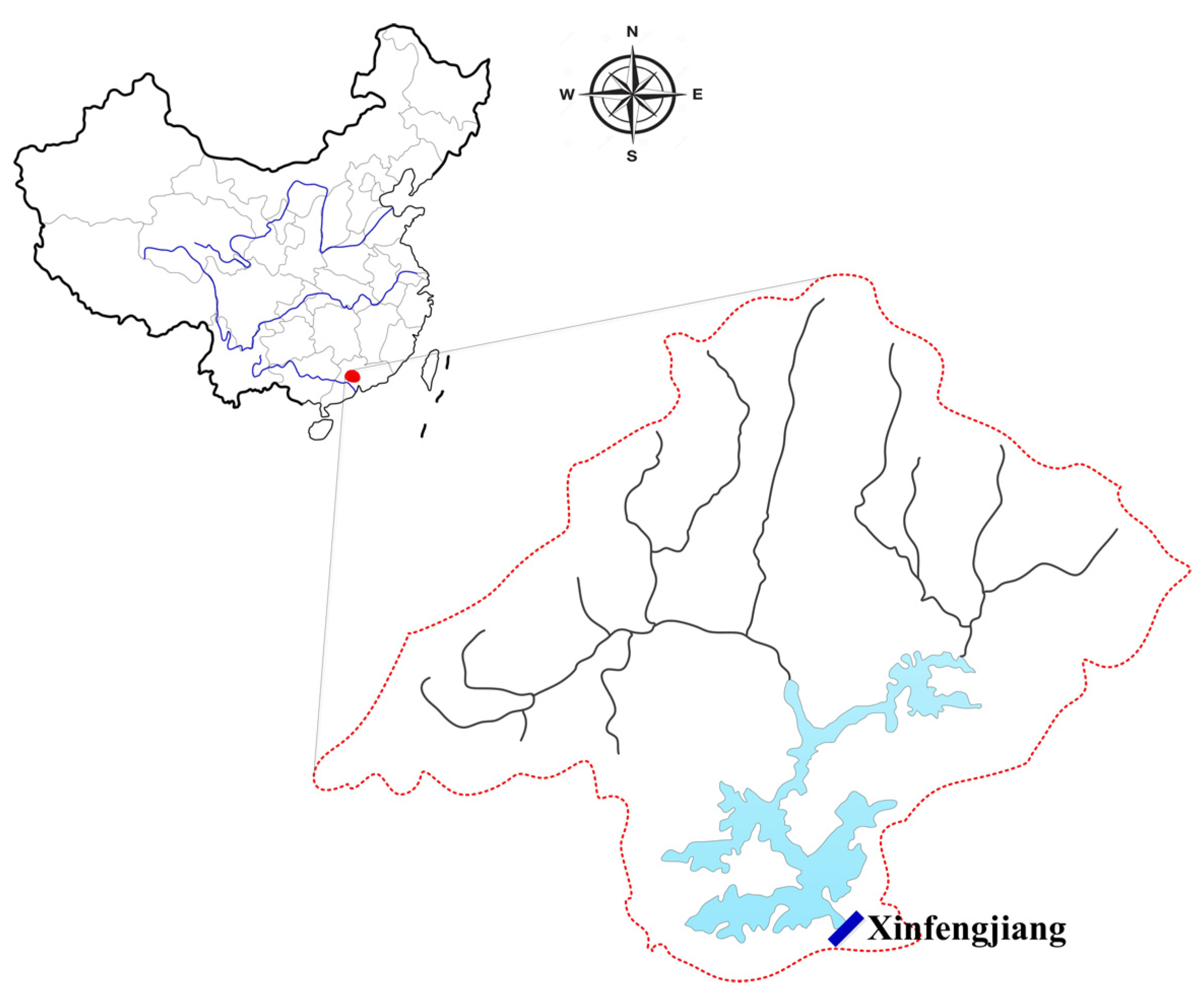
2.1. Study Area

The Pearl River (named Zhujiang in Chinese) is one of the world’s 25 largest rivers in terms of annual water discharge and sediment load [42]. The Pearl River originates from the Yunnan Plateau, crosses hill country and mountainous areas, and drains into the South China Sea. The Pearl River controls a drainage area of 450,000 km² and reaches a total length of 2400 km. The rainy season extends from April to September, followed by a dry season from October to March.

The Xinfengjiang reservoir, also known as Evergreen Lake, is within the boundaries of Guangdong Province, about six kilometers away from Heyuan City. Figure 1 shows the location of the study area and the Xinfengjiang reservoir. The reservoir is located on the outlet of Xinfengjiang River, which is a tributary of the East River. The East River is one of the three main tributaries of the Pearl River. The drainage area of the reservoir is 5740 km², which accounts for about one quarter of the East River Basin area. The average annual rainfall is about 1974.7 mm. The annual inflow at the dam site is about 192 m³/s. Since being put into production in October 1960, the reservoir began to play comprehensive benefit in power generation, flood control, navigation, water supply, etc. The reservoir is equipped with four units and its installed capacity arrives 302 million watts. The average annual energy generation is 0.99 billion kW·h. As the largest artificial reservoir with multi-year regulating storage in south China, the reservoir has the total capacity of 13.90 billion m³, where the dead storage capacity is 4.31 billion m³. Its normal water level is 116 m at non-flood season while the corresponding storage is 10.8 billion m³. Its flood control level is 114 m during the first half of flood season from 1 April to 30 June, whilst that is 115 m during the second half of flood season from 1 July to 30 September.

Figure 1. Location of the study area and Xinfengjiang reservoir.

Figure 1. Location of the study area and Xinfengjiang reservoir.

2.2. Division of Data

For meta-heuristic algorithms, such as ANN and SVM, the overtraining problem is likely to happen, which means that the models have excellent performance on the training data, but do not fit well to new data. In order to prevent the overtraining problem, Chau et al. (2005) suggested dividing the data into three subsets [5]: Training set for model training, testing set for monitoring the training process and validation set for model validation. Hence, in this study, the available data are divided into these above three data sets. The feasible monthly inflow data consists of 71 years (852 months) from 1944 to 2014 in Xinfengjiang reservoir. The first 55 years’ monthly inflow data were used as the training set while the last 16 years’ data were for validation. Moreover, of the training data, the first 40 years’ data was for model training, and the other 15 years’ data was for the purpose of confirming and validating the initial analysis.

It is hard to extrapolate for forecasting methods when the validation data contains variables beyond the range of training data. Table 1 shows the statistical parameters of various data sets, where X_mean, S_d, X_min, X_max, and R_ange respectively stand for the mean, standard deviation, minimum, maximum, and range of various data sets. We can find that the monthly inflow data for Xinfengjiang reservoir varies over a relative wide range from 9.3 to 1506 m³/s. The scope of the training data set includes that of testing and validation sets fully. The statistical parameters of the training set are close to the testing and validation sets. Hence, the data used for various data sets are representative of the same population, so there is no need to extrapolate beyond the range of the data for training.

Table 1. The information of various datasets in Xinfengjiang reservoir.

Datasets	Statistic
	Xmean	Sd	Xmin	Xmax	Range
Training set	204.1	14.3	9.3	1506.0	1496.7
Testing set	192.1	13.9	24.5	1300.2	1275.7
Validation set	176.3	13.3	22.3	1496.4	1474.1
Original data	195.3	14.0	9.3	1506.0	1496.7

Table 1. The information of various datasets in Xinfengjiang reservoir.

Datasets	Statistic
	Xmean	Sd	Xmin	Xmax	Range
Training set	204.1	14.3	9.3	1506.0	1496.7
Testing set	192.1	13.9	24.5	1300.2	1275.7
Validation set	176.3	13.3	22.3	1496.4	1474.1
Original data	195.3	14.0	9.3	1506.0	1496.7

2.3. Data Preprocessing

Moreover, according to Lin et al. in 2006 [41] and Wang et al. in 2009 [17], in consideration of the numerical difficulties caused by the large attribute values dominating the smaller ones, the normalization is an essential process for the raw data before applying the forecasting models to prediction in various data sets. Using the following Equation, the values have to be scaled to the range between 0 and 1 in the modeling process.

$$q_i^{\prime }=\frac{q_i-q_{\min }}{q_{\max }-q_{\min }}$$

(1)

where $q_i$ and $q_i^{\prime }$ is the original inflow value and scaled inflow value, respectively. $q_{\max }$ and $q_{\min }$ are the maximum and minimum of flow series, respectively.

3. Forecasting Methodology

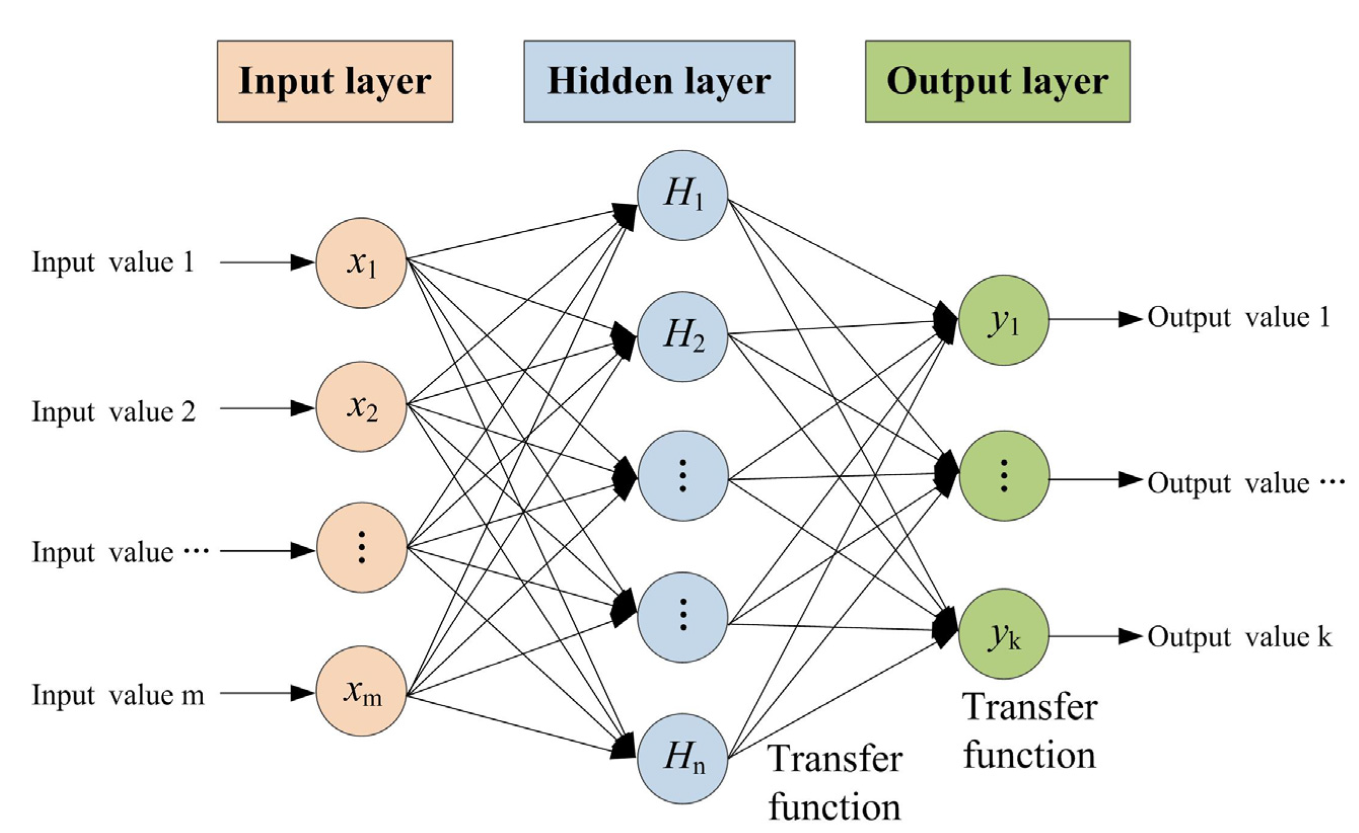
3.1. Artificial Neural Network (ANN)

As one of the most widely-used artificial intelligence methods, ANN has achieved great success in various fields by many researchers and scientists, like time-series prediction and simulation in water resources [5]. Through many investigations and practices, ANN has been proven that it is an efficient and reliable method in modeling nonlinear relationships between inputs and desired outputs in hydrologic time-series forecasting [16,17]. The ANN existence has much different kind of ways. ANN is commonly arranged in a series of layers composed of some close-connected processing neurons. Three-layer ANN, including one input layer, one hidden layer, and one output layer, is usually preferred in practical engineering applications because it can approximate almost any form of complex functional relationships between the inputs and desired outputs to arbitrary accuracy. Figure 2 shows the sketch map of a typical three-layer ANN. Every node usually gets an accumulated value by summing the values of its inputs multiplied by the corresponding weights associated with each interconnection, and then send the accumulated value to a nonlinear activation function to generate an output value which will be delivered to the following layer. Moreover, any one node of the previous layer is fully interconnected to all the nodes of the next layer, and there is no interconnection between any two nodes in the same layer.

Figure 2. Sketch map of a typical three-layer ANN.

Figure 2. Sketch map of a typical three-layer ANN.

The back propagation algorithm is one of the most popular learning methods for the ANN training. In addition, with our early research works, back propagation can be easily implemented and integrated in practical forecasting system [40]. Back propagation can be roughly divided into two stages: a feed-forward stage and a backward stage. In the feed-forward stage, the input information is delivered to the input layer, the hidden layer and the output layer in sequence, to obtain the output information. In the backward stage, the connection weights and thresholds are modified by the differences between the computed and desired output values. Without knowing the detailed information about the nature of the complex system, ANN can approach the optimal or near-optimal relationship between the input data set and the output data set by optimizing the structure of the network constantly. Mathematically, the network can be expressed as follow:

$$\mathit{Y}=f\left({\displaystyle \mathbf{\sum }\mathit{W}\mathit{X}+\mathit{B}}\right)$$

(2)

where Y is the output vector. f is the transfer function. W is the weight vector. X is the weight vector. B is the bias vector.

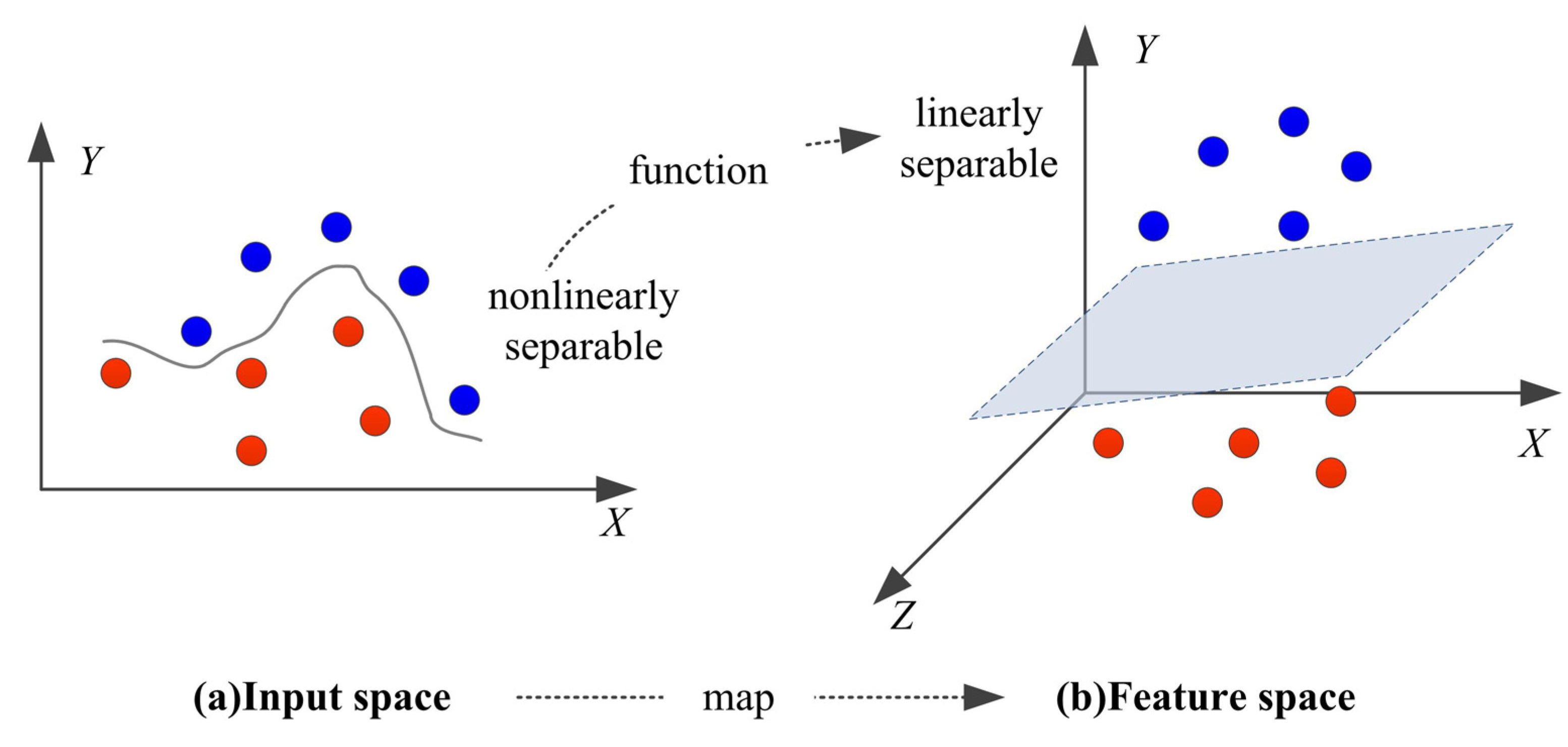
3.2. Support Vector Machine (SVM)

Support Vector Machine (SVM), proposed by Vapnik in 1995 [41], is a novel and useful tool for data classification and regression analysis. SVM is built on the basis of statistical learning methods and the structural risk minimization principle instead of the empirical risk minimization [19,31]. SVM can achieve a global optimum, in theory, and has been applied in many fields over the past decades, such as hydrology and computer science [43,44,45]. There are abundant papers about the detailed theory of SVM. Here, we introduce the information of SVM in brief, and the interested readers can find the detailed theory of SVM by referring to more papers. The fundamental idea of the SVM technique is to take advantage of a linear or nonlinear model to map the target input data into a higher dimensional characteristic space, so that the primary problem can be solved in the new space. For example, as shown in Figure 3, the problem of data classification which cannot be linearly separated on the plane may be linearly separable in the space with three or higher dimensions.

Figure 3. 2D input space mapping into 3D feature space to separate data linearly.

Figure 3. 2D input space mapping into 3D feature space to separate data linearly.

In SVM, the map model is usually defined as the kernel function to yield the inner products in the feature space and keep the calculated load reasonable. There are four kinds of commonly used kernel functions, including linear kernel, polynomial kernel, radial basis function (RBF) kernel, and sigmoid kernel [30,41]. Unlike the linear kernel, the RBF kernel can easily handle the non-linear relation between class labels and attributes. Compared with polynomial and sigmoid kernels, the RBF kernel has fewer tuning parameters, which reduces the complexity of model parameters selection. Moreover, the RBF kernel has good performance under general smoothness assumptions. In summary, the RBF kernel can improve the computational efficiency and enhance the generalization performance of SVM. Hence, the RBF kernel, as shown in Equation (3), is adopted as the kernel function in this study:

$$k\left(x_i,x\right)=\exp \left\{\frac{-{\Vert x-x_i\Vert }^2}{2{\text{σ}}^2}\right\}$$

(3)

where k represents the kernel function.

In the RBF kernel function, there are three parameters needed to be confirmed: the parameter C denotes the positive constant, the parameter ε represents the insensitive loss function, and the parameter σ denotes the Gaussian noise level of the standard deviation. Different parameter combinations can lead to large differences in the forecasting result. Thus, the combination of the three parameters has to be optimized, first, in order to improve the forecasting accuracy. Many methods are used to select these parameters, such as grid search technique, particle swarm optimization, and genetic algorithm. However, at present, no general guidelines are available for the parameter selection of SVM because each method has certain advantages and disadvantages. For example, the grid search technique has the advantages of simplicity and intuition but is more computationally expensive than other optimization techniques. As one of the most classic and popular evolutionary methods, genetic algorithm was widely employed to calibrate the combination of the three parameters due to its good robustness, adaptability, and simplicity, and satisfied results were also achieved in considerable research work. Therefore, for the better forecasting accuracy, we apply the GA to automatically choose the effective parameters combination of SVM kernel function.

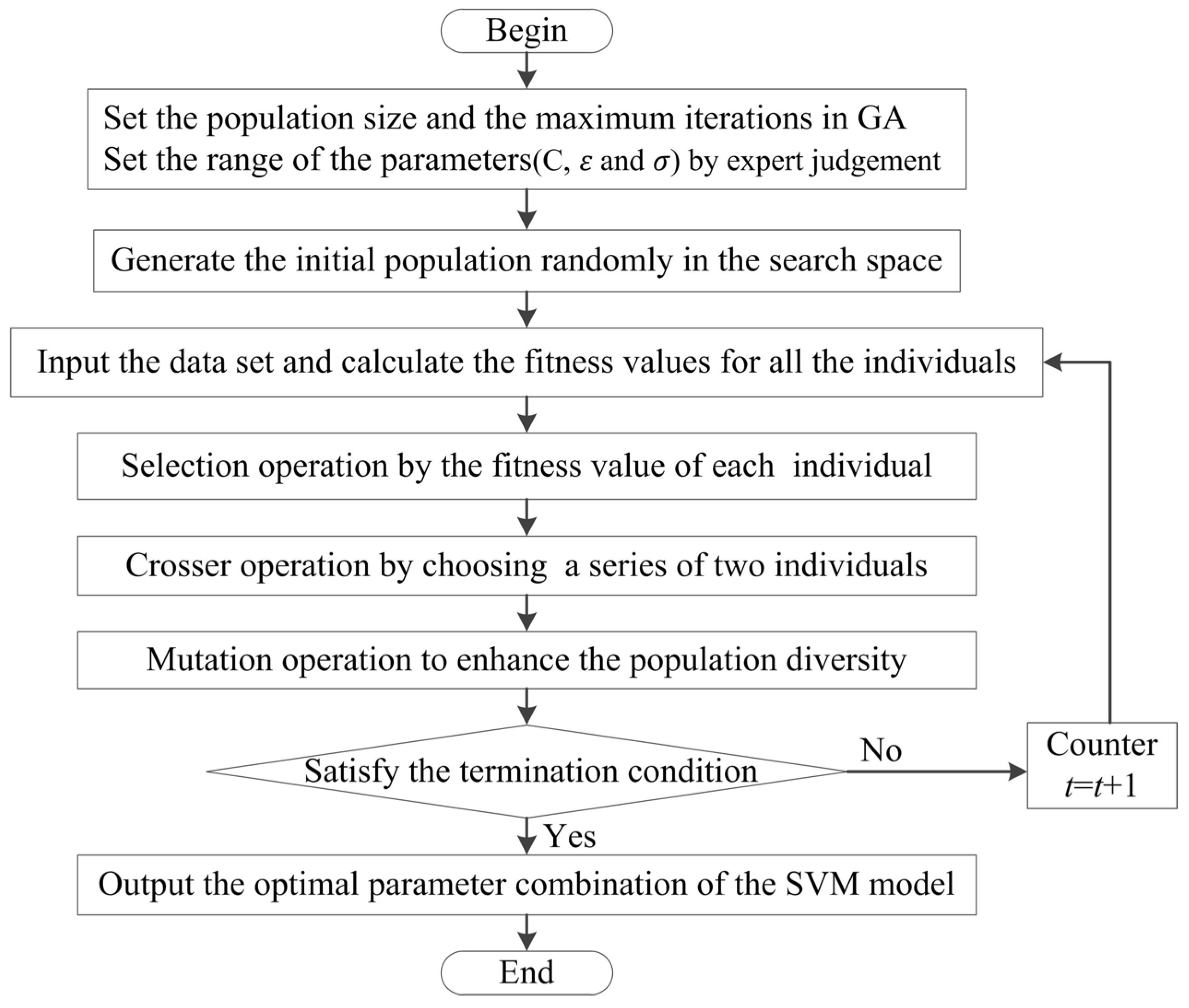
3.3. Genetic Algorithm (GA)

In nature, for the limited resources, the grim competition exists in different individuals of the same or different species, resulting in the fittest individuals outmatching the weaker ones [2,23]. GA is a classical heuristic search algorithm which mimics the thought of natural selection and genetic evolution in Darwin’s theory. By the power of evolution, GA can provide an efficient and robust search capability for the optimization problems associated with numerous complex constraints [34,35]. In GA, each potentially feasible or infeasible solution to the problem is encoded as a string of chromosomes. GA usually starts from a population of the given size which is generated randomly in the search space. Then GA evolves through three essential operators: A selection operator representing the survival of the fittest, a crossover operator equating to the mating between individuals, and a mutation operator increasing the diversity. On the basis of the initial population, GA calculates the fitness values of all the individuals, and the fitness value $F\left(\text{θ}\right)$ of the individual $\text{θ}$ uses the following formula:

$$F\left(\text{θ}\right)=\frac{1}{n}{\displaystyle \sum _{i=1}^n{\left[Y_i-SVM\left({\mathit{X}}_i,\text{θ}\right)\right]}^2}$$

(4)

where i represents the i-th data; n is the number of training data pairs; Y_i is the i-th observed data; X_i is the i-th input data vector; $SVM\left({\mathit{X}}_i,\text{θ}\right)$ represents the corresponding simulated value of SVM.

Then, the members with better fitness values are selected to form the population of the next generation. GA uses the crossover and mutation operators to enhance the population diversity. GA repeats the above-mentioned process until a certain terminal condition is met and the best individual represents the approximate optimal solution of the problem. Here, GA is employed to optimize the parameter combinations of the SVM model, and the objective is to minimize the fitness value of the optimal individual in the population, i.e., $\min F\left(\text{θ}\right)$. The flowchart is shown in Figure 4.

Figure 4. The flow chart of optimizing SVM using GA.

Figure 4. The flow chart of optimizing SVM using GA.

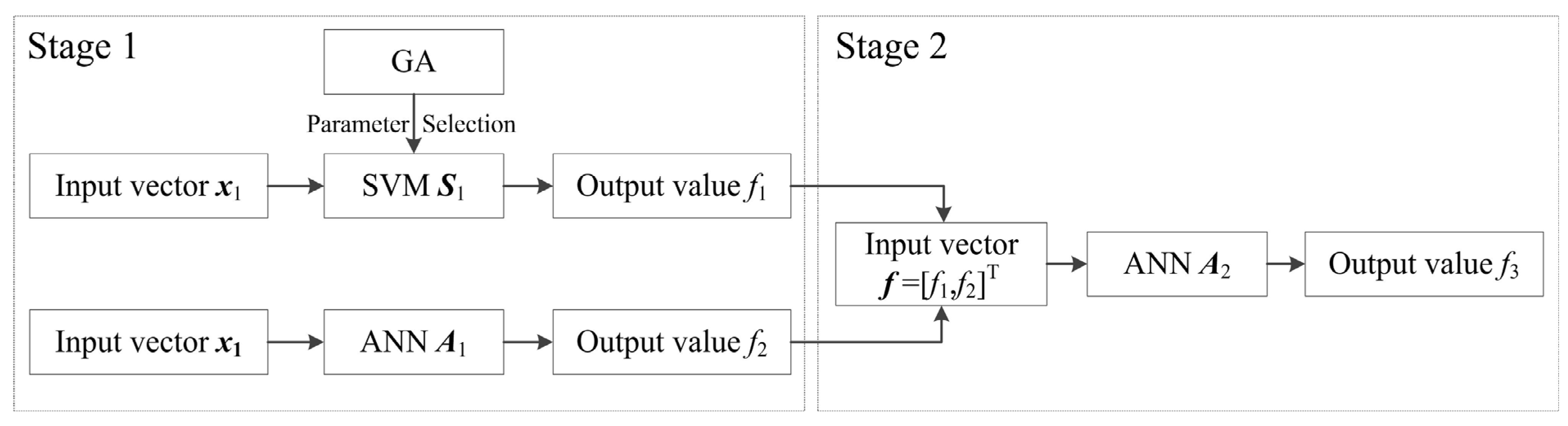
3.4. Hybrid Forecasting Method

The reservoir monthly inflow data series is controlled by a number of factors in the real world, including weather conditions, underlying surface, human activities, and others. These time-varying factors can introduce considerable uncertainty and noise, and affect the process of the inflow data series collection, pre-process, and prediction accuracy in the forecasting model. Hence, the reservoir monthly inflow data series usually presents the strong properties of randomness and volatility. On the one hand, a single forecasting model may reflect only one aspect of the character of the reservoir inflow in most cases so it is rather difficult to forecast the monthly inflow data accurately with one forecasting model because the bias or a large deviation always exists in the forecasting model. On the other hand, the results of two or more forecasting models can show the inflow characteristics from various perspectives. It is possible to further improve the prediction accuracy using different forecasting results. Therefore, to enhance the performance of the model, special treatment is required for the forecasting results to reduce the prediction errors of different models.

To deal with the problem of noise data caused by these aforementioned uncertain factors, this paper develops a hybrid forecast model based on ANN and SVM, which has many advantages discussed in the previous sections. The hybrid method is a two-stage process which can find an appropriate forecasting model to capture the complex relationship of the nonlinear system. First of all, the ANN A₁ and SVM S₁ forecasting model are driven to forecast the targeted reservoir inflow data, respectively, gaining two different forecasting results. Secondly, a new ANN model A₂ is built for the operational prediction, where the two different forecasting results of ANN and SVM are selected as the input variables and the real reservoir inflow data is used as the desired value. The two-stage forecasting process can be helpful to eliminate random errors of different models and improve the prediction ability to a certain degree. The framework of the proposed hybrid method is shown in Figure 5, and the process is described as below.

Step 1. Data processing. Divide the original valid monthly inflow data into various data sets, and these raw data are normalized to the preset range from 0 to 1.

Step 2. Model training in the first stage. Determine the structure of the ANN model A₁ and SVM model S₁, and use the abovementioned data to train both models, respectively, where GA is employed for the parameter selection of the SVM model S₁.

Step 3. Model training in the second stage. Determine the ANN model A₂ structure and use the processed data of the ANN model A₁ and SVM model S₁ as the input variables to train the model A₂.

Step 4. Model forecasting. The three optimized forecasting models are used to get the future values.

Figure 5. Sketch map of the hybrid method.

Figure 5. Sketch map of the hybrid method.

4. Statistical Measures

In this paper, the following five different types of error measurements are employed to evaluate the quality of the forecasting model. They are root mean square error (RMSE) and mean absolute error (MAE), mean absolute percentage error (MAPE), coefficient of correlation (R) and Nash-Sutcliffe (NS) efficiency coefficient. RMSE can be an arbitrary positive value and perform better when it is close to zero. MAE shows the degree of the absolute error between the forecasted and measured data. MAPE can express the relative absolute model error as a percentage. R, which ranges from −1 to 1, is a statistical measure of linear relationship between the observed and forecasted data. NS is less than or equal to 1, and has better forecasting capability when it is close to 1. The smaller the values of RMSE, MAE and MAPE are, the better the performance of the model shows. On the contrary, the larger the values of NS and R are, the better the forecasting model performs. The five criteria are calculated using the following Equations:

$$RMSE=\sqrt{\frac{1}{m}{\displaystyle \sum _{i=1}^m{\left(y_i-{\stackrel{⌢}{y}}_i\right)}^2}}$$

(5)

$$MAE=\frac{1}{m}{\displaystyle \sum _{i=1}^m\left|y_i-{\stackrel{⌢}{y}}_i\right|}$$

(6)

$$MAPE=\frac{1}{m}{\displaystyle \sum _{i=1}^m\left|\frac{y_i-{\stackrel{⌢}{y}}_i}{y_i}\right|}\times 100\%$$

(7)

$$R=\frac{{\displaystyle \sum _{i=1}^m\left[\left(y_i-\overline{y}\right)\left({\stackrel{⌢}{y}}_i-\tilde{y}\right)\right]}}{\sqrt{{\displaystyle \sum _{i=1}^m{\left(y_i-\overline{y}\right)}^2{\left({\stackrel{⌢}{y}}_i-\tilde{y}\right)}^2}}}$$

(8)

$$NS=1-\frac{{\displaystyle \sum _{i=1}^m{\left(y_i-{\stackrel{⌢}{y}}_i\right)}^2}}{{\displaystyle \sum _{i=1}^m{\left(y_i-\overline{y}\right)}^2}}$$

(9)

where $y_i$ and ${\stackrel{⌢}{y}}_i$ represent the i-th actual value and the i-th forecasted value of the forecasting model, respectively; $m$ is the total number of data set for comparison; $\overline{y}$ represents the average value of the observed data, $\overline{y}\text{=}\frac{1}{m}{\displaystyle \sum _{i=1}^m{y}_i}$; $\tilde{y}$ is the average value of the forecasted data, $\tilde{y}\text{=}\frac{1}{m}{\displaystyle \sum _{i=1}^m{\stackrel{⌢}{y}}_i}$.

5. Results and Discussion

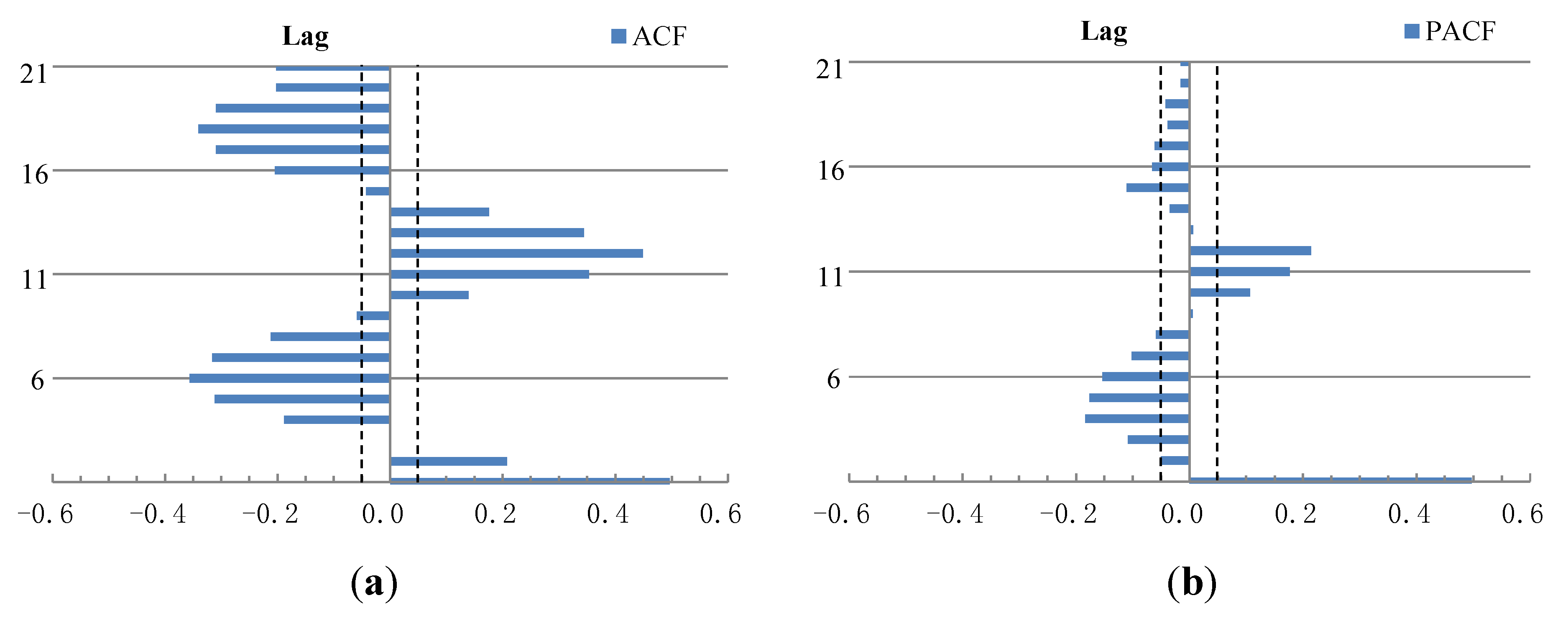
5.1. Input Variables Determination

Reasonable input variables can help capture the nonlinear features underlying the process and contribute to good model performance. For time-series forecasting, the autocorrelation function (ACF) and partial autocorrelation function (PACF) are two common parameters used to diagnose the order of the autoregressive process and determine the input vector of the model, too [17,41]. Figure 6 shows the ACF and PACF of the Xinfengjiang monthly inflow series with 95% confidence bands. Obviously, both ACF and PACF exhibit the peak value at lag 12, which indicates that twelve antecedent inflow values have the most useful information for the inflow forecasting. Hence, 12 antecedent inflow values are selected as the input vector based on autocorrelation coefficient analysis in this paper. The purpose of this study is to predict the inflow Q_t+1 at the time t+1. Hence, the relationship between the output and input variables can be expressed as the following Equation:

$$Q_{t+1}=R\left(Q_t,Q_{t-1},Q_{t-2},Q_{t-3},Q_{t-4},Q_{t-5},Q_{t-6},Q_{t-7},Q_{t-8},Q_{t-9},Q_{t-10},Q_{t-11}\right)$$

(10)

where $R$ denotes the nonlinear relationship, which are the corresponding model when ANN, SVM, and the hybrid method are used for inflow forecasting, respectively.

Figure 6. The (a) ACF and (b) PACF of Xinfengjiang monthly inflow series.

Figure 6. The (a) ACF and (b) PACF of Xinfengjiang monthly inflow series.

5.2. Development of Various Models

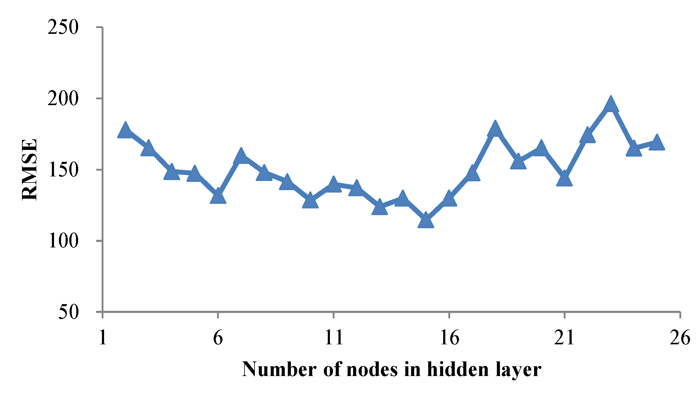
5.2.1. ANN Model A₁ Development

In the paper, we use a typical three-layer ANN model to forecast the monthly inflow in Xinfengjiang reservoir. All the neurons of hidden and output layers use the sigmoid transfer function. The twelve inputs and one output are applied to the ANN model, and all variables in the input and output data sets are normalized to the range between 0 and 1. The optimal network can be obtained using a trial and error procedure to train ANN models with various numbers of nodes in the hidden layer. As previously shown, the training data are further divided into the training set and the testing set. Based on the performances at different epochs, the cross-validation technique is used to select the optimum number of hidden neurons. Training is stopped when the error of the testing set starts to increase. Figure 7 shows the performances for the testing set with different hidden neurons from 2 to 25. When there are 15 neurons in the hidden layer, the testing error reached the minimum. Hence, the optimal ANN A₁ architecture is (12, 15, 1).

Figure 7. Performance of ANN model with different hidden nodes.

Figure 7. Performance of ANN model with different hidden nodes.

5.2.2. SVM Model S₁ Development

The setting of parameters plays an important role in the learning and generalization abilities of SVM. Larger search space is helpful for better parameters. Hence, the search scopes of three parameters are $C\in \left[2^{-5},2^{10}\right]$, $\text{σ}\in \left[2^{-5},2^{10}\right]$ and $\text{ε}\in \left[2^{-13},2^5\right]$. GA is used for the parameter selection of the SVM model. The SVM parameters are directly encoded using real value data in the chromosomes of the GA. The maximum iteration of GA is 500 and the population size is set to 300. Similar to the ANN model, the same data sets are used to optimize the parameters of SVM. To obtain more appropriate parameters, the overall process is repeated five times and the best model is selected as the final forecasting model. Table 2 displays the performance statistics of SVM models. The results indicate that, in the fourth run, SVM model with the optimal parameters (C, ε, σ) = (9.425, 0.823, 0.081) behaved the best and should be selected as the forecast model for Xinfengjiang reservoir.

Table 2. The performance statistics of SVM models using GA over five runs.

Trial No.	Optimal Parameters (C, ε, σ)	Training					Validation
		RMSE	MAPE	MAE	NS	R	RMSE	MAPE	MAE	NS	R
1	(10.653, 1.032, 0.078)	151.00	59.19	87.85	0.49	0.70	153.90	70.23	93.03	0.42	0.64
2	(9.827, 0.435, 0.064)	144.82	54.29	85.60	0.53	0.73	133.07	61.87	82.54	0.56	0.75
3	(2.783, 0.678, 0.125)	152.46	61.54	88.08	0.48	0.69	152.51	66.38	89.44	0.43	0.65
4	(9.425, 0.823, 0.081)	118.66	70.48	82.44	0.68	0.83	96.60	75.73	74.36	0.77	0.89
5	(11.803, 1.254, 0.708)	147.80	64.17	88.98	0.51	0.71	154.22	74.28	94.58	0.41	0.65

Table 2. The performance statistics of SVM models using GA over five runs.

Trial No.	Optimal Parameters (C, ε, σ)	Training					Validation
		RMSE	MAPE	MAE	NS	R	RMSE	MAPE	MAE	NS	R
1	(10.653, 1.032, 0.078)	151.00	59.19	87.85	0.49	0.70	153.90	70.23	93.03	0.42	0.64
2	(9.827, 0.435, 0.064)	144.82	54.29	85.60	0.53	0.73	133.07	61.87	82.54	0.56	0.75
3	(2.783, 0.678, 0.125)	152.46	61.54	88.08	0.48	0.69	152.51	66.38	89.44	0.43	0.65
4	(9.425, 0.823, 0.081)	118.66	70.48	82.44	0.68	0.83	96.60	75.73	74.36	0.77	0.89
5	(11.803, 1.254, 0.708)	147.80	64.17	88.98	0.51	0.71	154.22	74.28	94.58	0.41	0.65

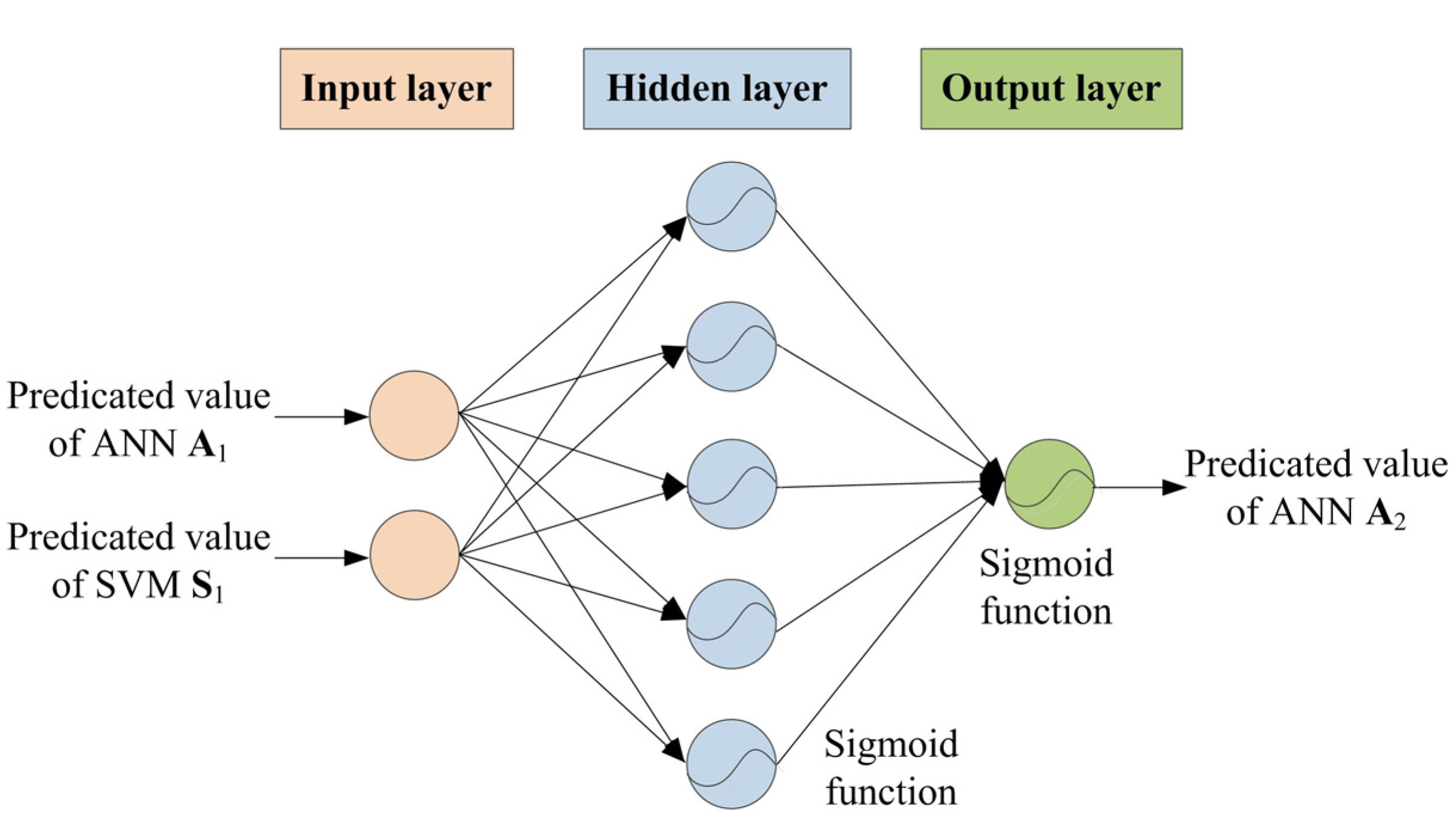
5.2.3. ANN Model A₂ Development

The two above models, ANN and SVM, are executed to respectively obtain the predicted data. The ANN model A₂ uses the results of both ANN model A₁ and SVM model S₁ as its input variables. There are two inputs and one output in the model. A typical three-layer network is used. The sigmoid transfer function is used in all neurons of the hidden layer and the output layer. To ensure the generalization, all variables are normalized, and a trial-and-error process is repeated to determine the optimal hidden layer nodes. The number of neuron in the hidden layer vary from two to nine, and all the statistical indexes of different network structures are recorded and compared during the calculation procedure. Finally, the optimal neural network adopted was (2, 5, 1), as shown in Figure 8, which was selected as the final forecasting model.

Figure 8. The optimal structure for ANN model A₂.

Figure 8. The optimal structure for ANN model A₂.

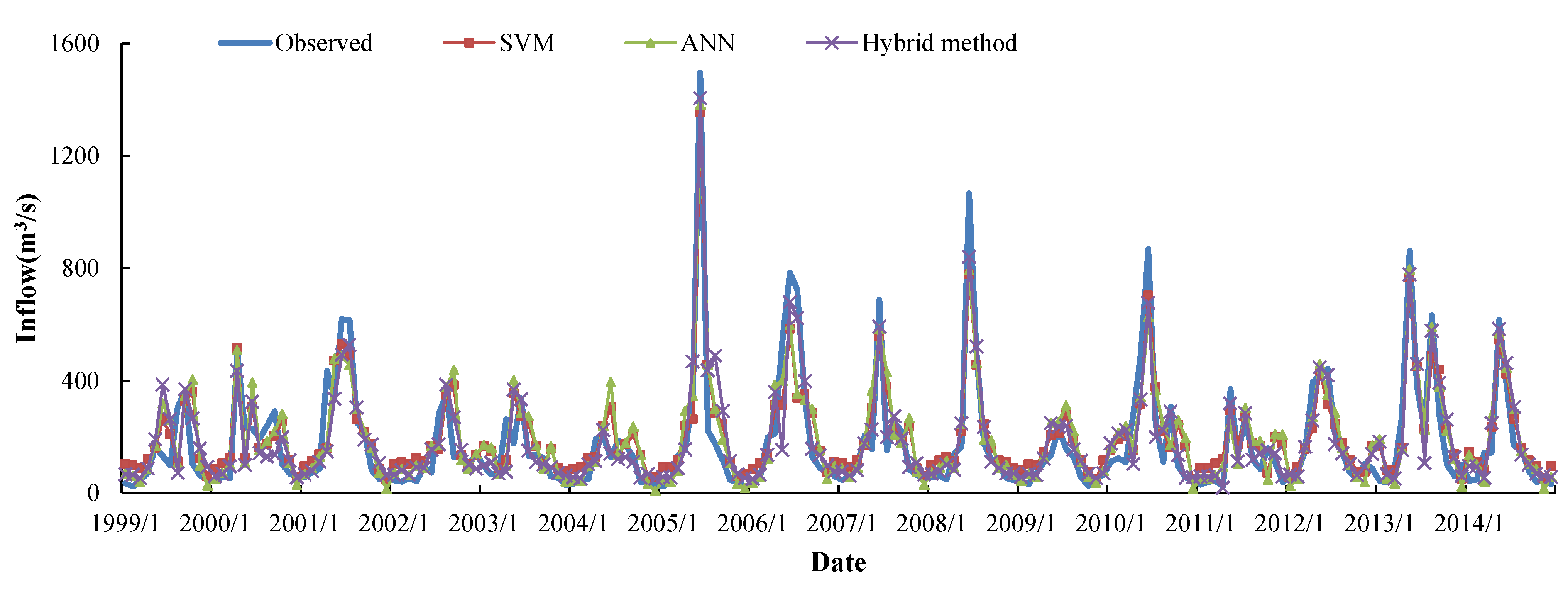
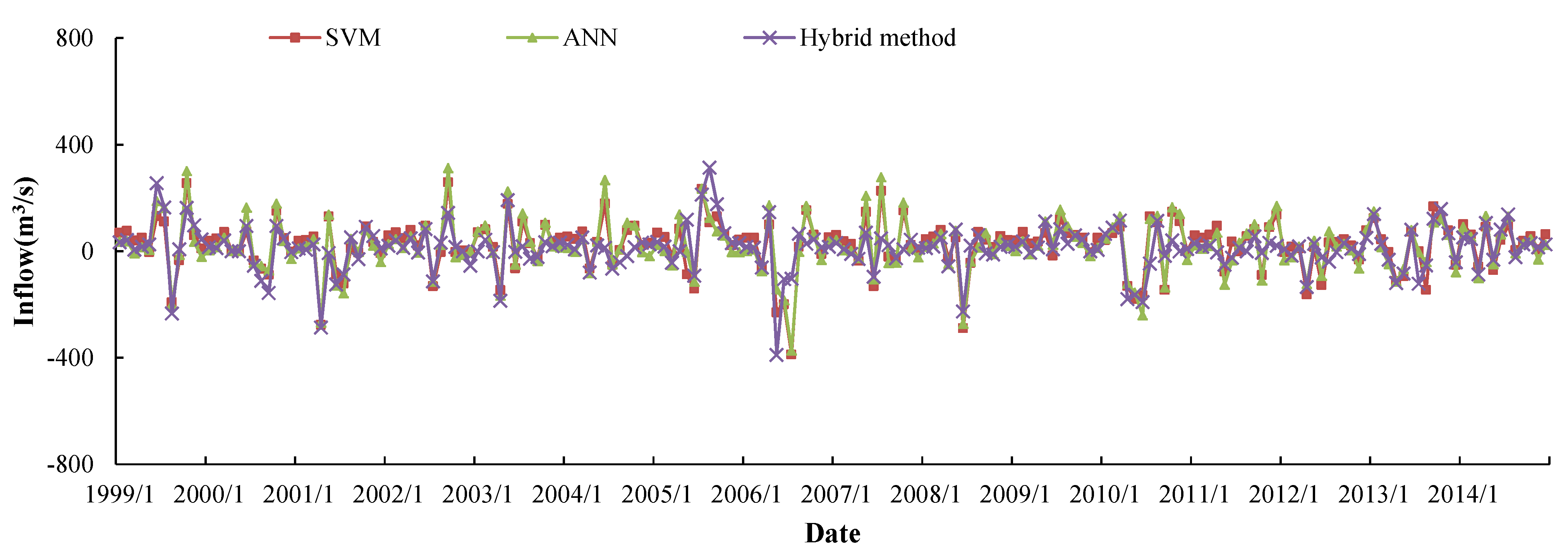
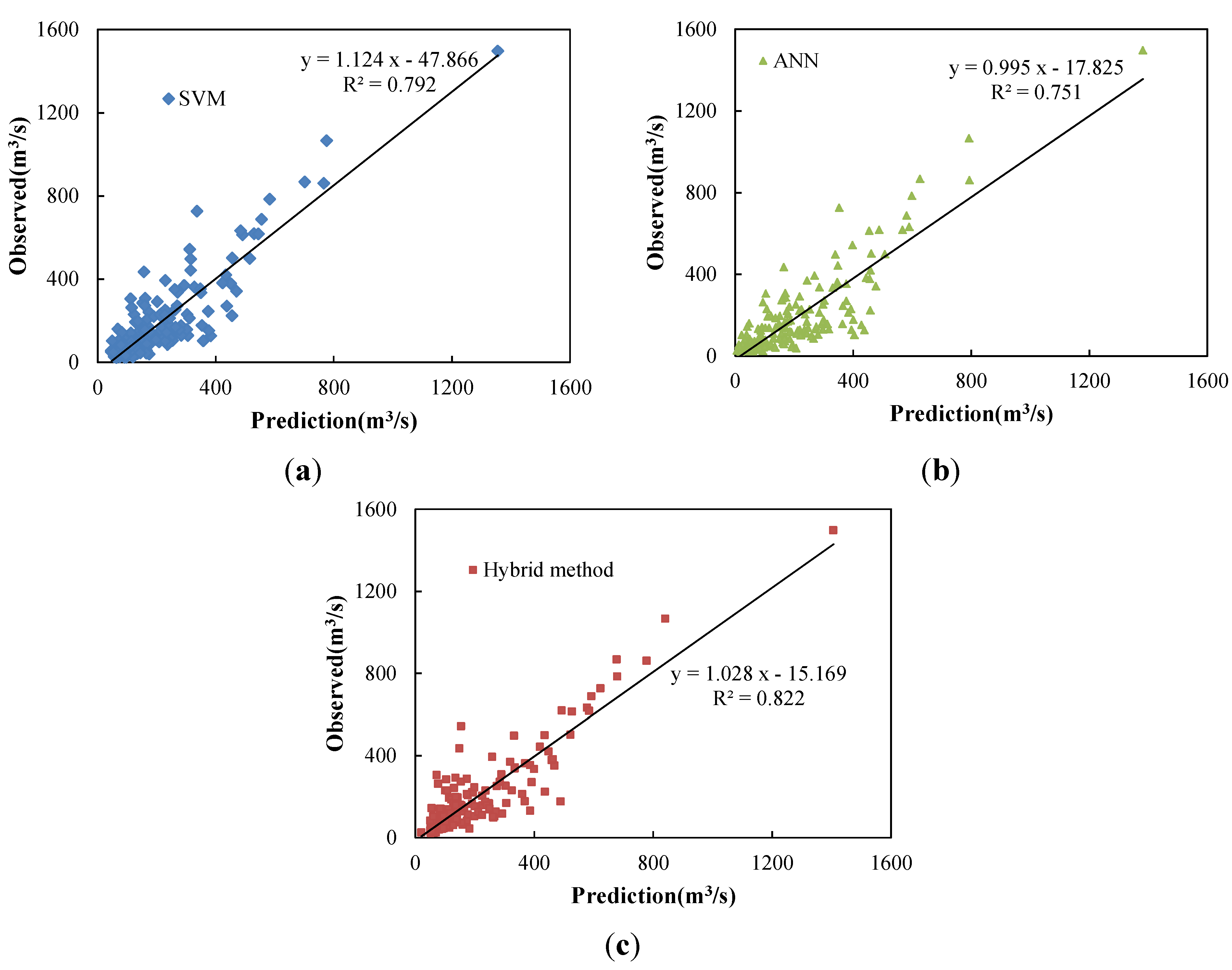
5.3. Comparison and Discussion

For the sake of comparison, three forecasting methods, namely ANN, SVM, and the hybrid method are tested under the same experimental conditions. The same data sets are used to verify the performance of various forecasting models in the same way. Every one-month step is predicted and compared with the actual inflow data to calculate the errors. The process is repeated over the whole time series, and then the average errors of all the months data are calculated. The obtained appropriate architectures of the ANN model A₁ and A₂ for Xinfengjiang reservoir are (12, 15, 1) and (2, 5, 1), respectively. Moreover, using GA for parameter selection, the SVM model with parameters (C, ε, σ) = (9.425, 0.823, 0.081) is the forecasting model for Xinfengjiang reservoir.

Table 3 summarizes the statistical values of the three models in both training and validation periods. We can efficiently execute the analysis of the predictive ability of different models for Xinfengjiang reservoir. When compared to the original ANN and SVM, the hybrid method can produce better and closer prediction accuracy in term of all five measures during various periods. In the training period, the hybrid method achieves 19.21%, 24.26%, and 31.50% reduction in the RMSE, MAE, and MAPE values of SVM, respectively. Compared with ANN model, improvements of the hybrid model’s forecast results regarding the R and NS were approximately 7.23% and 16.18%, respectively. In the validation period, the hybrid method can make 16.03%, 20.63%, and 21.83% improvements of the ANN forecast results related to the RMSE, MAE, and MAPE, respectively. The R and NS values of the hybrid method increase by 2.25% and 6.49% when compared with the SVM model, respectively. Thus, the above analysis indicates that the proposed method is able to obtain the best results in terms of all five different evaluation measures during both training and validation periods. The hybrid method starts the operational prediction using the processed data with more abundant information rather than original input vector, which help the forecasting model raise the cognitive level for the characteristics of time-variable monthly inflow data. By combining advantages of ANN and SVM, the hybrid method can effectively eliminate the noise of the original hydrological series. Therefore, the hybrid method can improve the forecasting accuracy of the monthly inflow data from Xinfengjiang reservoir.

Table 3. Model statistics of three models for Xinfengjiang reservoir.

Models	Training					Validation
	RMSE	MAPE	MAE	NS	R	RMSE	MAPE	MAE	NS	R
SVM	118.66	70.48	82.44	0.68	0.83	96.60	75.73	74.36	0.77	0.89
ANN	118.60	55.20	79.73	0.68	0.83	102.09	63.68	73.49	0.74	0.87
Hybrid Method	95.86	48.28	62.44	0.79	0.89	85.72	49.78	58.33	0.82	0.91

Table 3. Model statistics of three models for Xinfengjiang reservoir.

Models	Training					Validation
	RMSE	MAPE	MAE	NS	R	RMSE	MAPE	MAE	NS	R
SVM	118.66	70.48	82.44	0.68	0.83	96.60	75.73	74.36	0.77	0.89
ANN	118.60	55.20	79.73	0.68	0.83	102.09	63.68	73.49	0.74	0.87
Hybrid Method	95.86	48.28	62.44	0.79	0.89	85.72	49.78	58.33	0.82	0.91

Figure 9 and Figure 10 respectively shows a comparison of forecasted versus observed values, and errors by predicted minus observed of the three models for the Xinfengjiang reservoir in the validation period. Figure 11 shows the scatterplots of observed inflow data versus forecast inflow of the three prediction models. Figure 9 demonstrates that the simulation results accord well with the observed results and the three models can capture the whole trend of the data series in the validation stage. The plots of errors in Figure 10 illustrate that a certain underestimation or overestimation exists in the monthly inflow predication value of each model. Due to the small magnitude and frequent occurrences of the low inflow pattern, all three models have slightly smaller errors and better generalization in these regions than high inflow pattern. The results are consistent with that in Table 3 and Table 4. The linear trend line of the hybrid method in Figure 11 has the biggest R-squared value, which means that the trend line is closest to the perfect 45-degree line. From Figure 9, Figure 10 and Figure 11, it can be observed that, when employed for monthly inflow data prediction, three models can achieve satisfactory performances for simulating the monthly inflow of Xinfengjiang reservoir, the hybrid method has high consistency and good stability, and performs better than SVM and ANN models in different inflow levels. To sum up, in the hybrid method, the ANN and SVM models are first used for the structure identification of different resolution in the hydrological time series, and then a newly-built ANN model is constructed for the refined prediction so as to enhance the prediction capability of the forecasting model. Therefore, the proposed method has satisfied performance when predicting the monthly inflow data series.

Figure 9. Comparison of forecasted versus observed data by various methods during the validation period.

Figure 9. Comparison of forecasted versus observed data by various methods during the validation period.

Figure 10. Comparison of errors by various methods during the validation period.

Figure 10. Comparison of errors by various methods during the validation period.

Figure 11. Scatter plots of forecasted versus observed data by various methods during the validation period. (a) SVM; (b) ANN and (c) Hybrid method.

Figure 11. Scatter plots of forecasted versus observed data by various methods during the validation period. (a) SVM; (b) ANN and (c) Hybrid method.

Table 4 lists the peak flow estimation of SVM, ANN, and the hybrid method for Xinfengjiang reservoir during the validation period. The maximum observed peak inflow is 1496.4 m³/s in June 2015, while the forecast value of the SVM, ANN, and hybrid method are 1355.5, 1381.3, and 1405.7 m³/s, about 9.4%, 7.7% and 6.1% underestimation, respectively. For the second maximum peak inflow in June 2008, the SVM, ANN, and the hybrid method can obtain 776.5, 792.3, and 840.5 m³/s instead of the observed 1066 m³/s, about 27.2%, 25.7% and 21.2% underestimation, respectively. Moreover, for the 16 peak flows, the absolute average relative error of the SVM, ANN, and the hybrid method are 15.2%, 15.5% and 10.6%, respectively. Thus, it can be concluded that for peak inflow prediction, the hybrid method can obtain better forecast precision than SVM and ANN, while there is no significant difference between ANN and SVM.

Table 4. Peak flow estimates of three models for Xinfengjiang reservoir during the validation period.

Peak No.	Date	Observed	Forecast Peak			Relative Error (%)
		Peak	SVM	ANN	Hybrid Method	SVM	ANN	Hybrid Method
1	1999/9	362.0	327.9	346.9	369.5	−9.4	−4.2	2.1
2	2000/4	497.9	516.0	507.5	434.9	3.6	1.9	−12.7
3	2001/6	618.1	530.3	488.4	492.9	−14.2	−21.0	−20.3
4	2002/8	352.6	349.1	376.7	386.2	−1.0	6.8	9.5
5	2003/6	336.2	272.0	285.6	334.4	−19.1	−15.1	−0.5
6	2004/5	202.8	237.3	236.8	225.8	17.0	16.8	11.3
7	2005/6	1496.4	1355.5	1381.3	1405.7	−9.4	−7.7	−6.1
8	2006/6	783.8	583.2	598.1	679.5	−25.6	−23.7	−13.3
9	2007/6	687.5	555.7	581.4	592.1	−19.2	−15.4	−13.9
10	2008/6	1066.0	776.5	792.3	840.5	−27.2	−25.7	−21.2
11	2009/6	228.2	211.5	252.4	236.1	−7.3	10.6	3.5
12	2010/6	867.5	701.4	626.7	677.5	−19.2	−27.8	−21.9
13	2011/5	369.6	293.5	244.1	319.3	−20.6	−34.0	−13.6
14	2012/6	442.3	315.6	348.7	419.6	−28.6	−21.2	−5.1
15	2013/5	860.9	766.5	794.2	778.3	−11.0	−7.7	−9.6
16	2014/5	616.2	544.8	567.0	584.9	−11.6	−8.0	−5.1
Average (absolute)						15.2	15.5	10.6

Table 4. Peak flow estimates of three models for Xinfengjiang reservoir during the validation period.

Peak No.	Date	Observed	Forecast Peak			Relative Error (%)
		Peak	SVM	ANN	Hybrid Method	SVM	ANN	Hybrid Method
1	1999/9	362.0	327.9	346.9	369.5	−9.4	−4.2	2.1
2	2000/4	497.9	516.0	507.5	434.9	3.6	1.9	−12.7
3	2001/6	618.1	530.3	488.4	492.9	−14.2	−21.0	−20.3
4	2002/8	352.6	349.1	376.7	386.2	−1.0	6.8	9.5
5	2003/6	336.2	272.0	285.6	334.4	−19.1	−15.1	−0.5
6	2004/5	202.8	237.3	236.8	225.8	17.0	16.8	11.3
7	2005/6	1496.4	1355.5	1381.3	1405.7	−9.4	−7.7	−6.1
8	2006/6	783.8	583.2	598.1	679.5	−25.6	−23.7	−13.3
9	2007/6	687.5	555.7	581.4	592.1	−19.2	−15.4	−13.9
10	2008/6	1066.0	776.5	792.3	840.5	−27.2	−25.7	−21.2
11	2009/6	228.2	211.5	252.4	236.1	−7.3	10.6	3.5
12	2010/6	867.5	701.4	626.7	677.5	−19.2	−27.8	−21.9
13	2011/5	369.6	293.5	244.1	319.3	−20.6	−34.0	−13.6
14	2012/6	442.3	315.6	348.7	419.6	−28.6	−21.2	−5.1
15	2013/5	860.9	766.5	794.2	778.3	−11.0	−7.7	−9.6
16	2014/5	616.2	544.8	567.0	584.9	−11.6	−8.0	−5.1
Average (absolute)						15.2	15.5	10.6

6. Conclusions

In order to improve the forecasting accuracy of monthly inflow in Xinfengjiang reservoir, this paper develops a hybrid forecasting method based on artificial neural network (ANN), support vector machine (SVM) and genetic algorithm (GA) to forecast the monthly inflow data series. The forecasting process of the hybrid method can be divided into two stages. In the first stage, SVM and ANN are used to identify the complex nonlinear characteristic correlation between the input and the output data, and GA is implemented to seek for the parameter combination of the SVM model. In the second stage, for better forecasting accuracy, the results of the SVM and ANN are taken as input variables of a new ANN model, and the corresponding predicative results of the new ANN model is the final forecasting inflow value. Three different models, ANN, SVM, and the hybrid prediction model are applied to forecast the monthly inflow data from Xinfengjiang dam reservoir of Pearl River Basin in China, and five statistical measures are employed to evaluate the performances of these various models. From the detailed analysis in this work, it can be concluded that these three models can obtain the satisfactory forecasting accuracy for the monthly inflow data in Xinfengjiang reservoir, and the proposed hybrid method significantly outperforms the traditional ANN and SVM. Therefore, the hybrid forecasting method proposed in this paper can capture the potential information and relationship of the monthly inflow data series and will be helpful for Xinfengjiang reservoir managers to obtain more accurate and stable forecasting results. However, due to the limitation of the authors’ time and energy, there are, undoubtedly, some defects needed to deepen in further research work. For example, only ANN and SVM are compared and considered in the present study for simplicity, more approaches can be considered and involved in the hybrid method, to enhance the generalizability of the forecasting model. In addition, the accuracy and applicability of the hybrid method in different reservoirs’ monthly or other-scale inflow under different climate conditions can also be further examined.

References

1. Zhao, T.; Zhao, J. Joint and respective effects of long and short-term forecast uncertainties on reservoir operations. J. Hydrol. 2014, 517, 83–94. [Google Scholar] [CrossRef]
2. Chiu, Y.C.; Chang, L.C.; Chang, F.J. Using a hybrid genetic algorithm-simulated annealing algorithm for fuzzy programming of reservoir operation. Hydrol. Process. 2007, 21, 3162–3172. [Google Scholar] [CrossRef]
3. Karamouz, M.; Ahmadi, A.; Moridi, A. Probabilistic reservoir operation using bayesian stochastic model and support vector machine. Adv. Water Resour. 2009, 32, 1588–1600. [Google Scholar] [CrossRef]
4. Lian, J.; Yao, Y.; Ma, C.; Guo, Q. Reservoir operation rules for controlling algal blooms in a tributary to the impoundment of three gorges dam. Water 2014, 6, 3200–3223. [Google Scholar] [CrossRef]
5. Chau, K.W.; Wu, C.L.; Li, Y.S. Comparison of several flood forecasting models in Yangtz River. J. Hydrol. Eng. 2005, 10, 485–491. [Google Scholar] [CrossRef]
6. Liu, P.; Lin, K.; Wei, X. A two-stage method of quantitative flood risk analysis for reservoir real-time operation using ensemble-based hydrologic forecasts. Stoch. Env. Res. Risk A 2014, 29, 803–813. [Google Scholar] [CrossRef]
7. Chau, K.W.; Wu, C.A. Hybrid model coupled with singular spectrum analysis for daily rainfall prediction. J. Hydroinform. 2010, 12, 458–473. [Google Scholar] [CrossRef]
8. Cheng, C.T.; Lin, J.Y.; Sun, Y.G.; Chau, K.W. Long-term prediction of discharges in Manwan hydropower using adaptive-network-based fuzzy inference systems models. Lect. Notes Comput. Sci. 2005, 3612, 1152–1161. [Google Scholar]
9. Fleming, S.W.; Weber, F.A. Detection of long-term change in hydroelectric reservoir inflows: Bridging theory and practice. J. Hydrol. 2012, 470, 36–54. [Google Scholar] [CrossRef]
10. Wu, C.L.; Chau, K.W.; Li, Y.S. Methods to improve neural network performance in daily flows prediction. J. Hydrol. 2009, 372, 80–93. [Google Scholar] [CrossRef]
11. Lund, J.R. Flood Management in California. Water 2012, 4, 157–169. [Google Scholar] [CrossRef]
12. Muttil, N.; Chau, K.W. Machine learning paradigms for selecting ecologically significant input variables. Eng. Appl. Artif. Intell. 2007, 20, 735–744. [Google Scholar] [CrossRef] [Green Version]
13. Coulibaly, P.; Haché, M.; Fortin, V.; Bobée, B. Improving daily reservoir inflow forecasts with model combination. J. Hydrol. Eng. 2005, 10, 91–99. [Google Scholar] [CrossRef]
14. Zhu, T.; Lund, J.R.; Jenkins, M.W.; Marques, G.F.; Ritzema, R.S. Climate change, urbanization, and optimal long-term floodplain protection. Water Resour. Res. 2007, 43, 122–127. [Google Scholar] [CrossRef]
15. Wu, C.L.; Chau, K.W. Data-driven models for monthly streamflow time series prediction. Eng. Appl. Artif. Intell. 2010, 23, 1350–1367. [Google Scholar] [CrossRef]
16. Valipour, M.; Banihabib, M.E.; Behbahani, S.M.R. Comparison of the ARMA, ARIMA and the autoregressive artificial neural network models in forecasting the monthly inflow of Dez dam reservoir. J. Hydrol. 2013, 476, 433–441. [Google Scholar] [CrossRef]
17. Wang, W.C.; Chau, K.W.; Cheng, C.T.; Qiu, L. A comparison of performance of several artificial intelligence methods for forecasting monthly discharge time series. J. Hydrol. 2009, 374, 294–306. [Google Scholar] [CrossRef]
18. Taormina, R.; Chau, K.W. Neural network river forecasting with multi-objective fully informed particle swarm optimization. J. Hydroinform. 2015, 17, 99–113. [Google Scholar] [CrossRef]
19. Lin, G.F.; Chen, G.R.; Huang, P.Y. Effective typhoon characteristics and their effects on hourly reservoir inflow forecasting. Adv. Water Resour. 2010, 33, 887–898. [Google Scholar] [CrossRef]
20. Demirel, M.C.; Venancio, A.; Kahya, E. Flow forecast by SWAT model and ANN in Pracana basin, Portugal. Adv. Eng. Softw. 2009, 40, 467–473. [Google Scholar] [CrossRef]
21. Saeidifarzad, B.; Nourani, V.; Aalami, M.; Chau, K.W. Multi-site calibration of linear reservoir based geomorphologic rainfall-runoff models. Water 2014, 6, 2690–2716. [Google Scholar] [CrossRef]
22. Chen, W.; Chau, K.W. Intelligent manipulation and calibration of parameters for hydrological models. Int. J. Environ. Pollut. 2006, 28, 432–447. [Google Scholar] [CrossRef]
23. Cheng, C.T.; Ou, C.P.; Chau, K.W. Combining a fuzzy optimal model with a genetic algorithm to solve multi-objective rainfall-runoff model calibration. J. Hydrol. 2002, 268, 72–86. [Google Scholar] [CrossRef]
24. Gupta, H.V.; Kling, H.; Yilmaz, K.K.; Martinez, G.F. Decomposition of the mean squared error and NSE performance criteria: Implications for improving hydrological modelling. J. Hydrol. 2009, 377, 80–91. [Google Scholar] [CrossRef]
25. Sattari, M.T.; Yurekli, K.; Pal, M. Performance evaluation of artificial neural network approaches in forecasting reservoir inflow. Appl. Math. Model. 2012, 36, 2649–2657. [Google Scholar] [CrossRef]
26. Maier, H.R.; Dandy, G.C. Neural networks for the prediction and forecasting of water resources variables: A review of modeling issues and applications. Environ. Modell. Softw. 2000, 15, 101–124. [Google Scholar] [CrossRef]
27. Taormina, R.; Chau, K.W.; Sethi, R. Artificial neural network simulation of hourly groundwater levels in a coastal aquifer system of the venice lagoon. Eng. Appl. Artif. Intell. 2012, 25, 1670–1676. [Google Scholar] [CrossRef]
28. Kisi, O.; Cimen, M. A wavelet-support vector machine conjunction model for monthly streamflow forecasting. J. Hydrol. 2011, 399, 132–140. [Google Scholar] [CrossRef]
29. Yang, J.S.; Yu, S.P.; Liu, G.M. Multi-step-ahead predictor design for effective long-term forecast of hydrological signals using a novel wavelet neural network hybrid model. Hydrol. Earth Syst. Sci. 2013, 17, 4981–4993. [Google Scholar] [CrossRef]
30. Noori, R.; Karbassi, A.R.; Moghaddamnia, A.; Han, D.; Zokaei-Ashtiani, M.H.; Farokhnia, A.; Gousheh, M.G. Assessment of input variables determination on the SVM model performance using PCA, Gamma test, and forward selection techniques for monthly stream flow prediction. J. Hydrol. 2011, 40, 177–189. [Google Scholar] [CrossRef]
31. Lin, G.F.; Chen, G.R.; Wu, M.C.; Chou, Y.C. Effective forecasting of hourly typhoon rainfall using support vector machines. Water Resour. Res. 2009, 45, 560–562. [Google Scholar] [CrossRef]
32. Bazartseren, B.; Hildebrandt, G.; Holz, K.P. Short-term water level prediction using neural networks and neuro-fuzzy approach. Neurocomputing 2003, 55, 439–450. [Google Scholar] [CrossRef]
33. Coulibaly, P.; Anctil, F.; Bobee, B. Daily reservoir inflow forecasting using artificial neural networks with stopped training approach. J. Hydrol. 2000, 230, 244–257. [Google Scholar] [CrossRef]
34. Su, J.; Wang, X.; Zhao, S.; Chen, B.; Li, C.; Yang, Z. A structurally simplified hybrid model of genetic algorithm and support vector machine for prediction of chlorophyll a in reservoirs. Water 2015, 7, 1610–1627. [Google Scholar] [CrossRef]
35. Kuo, J.T.; Wang, Y.Y.; Lung, W.S. A hybrid neural-genetic algorithm for reservoir water quality management. Water Res. 2006, 40, 1367–1376. [Google Scholar] [CrossRef] [PubMed]
36. Guo, Z.H.; Wu, J.; Lu, H.Y.; Wang, J.Z. A case study on a hybrid wind speed forecasting method using bp neural network. Knowl. Based Syst. 2011, 24, 1048–1056. [Google Scholar] [CrossRef]
37. Thirumalaiah, K.; Deo, M.C. River stage forecasting using artificial neural networks. J. Hydrol. Eng. 1998, 3, 26–32. [Google Scholar] [CrossRef]
38. Alvisi, S.; Mascellani, G.; Franchini, M.; Bardossy, A. Water level forecasting through fuzzy logic and artificial neural network approaches. Hydrol. Earth Syst. Sci. 2006, 10, 1–17. [Google Scholar] [CrossRef]
39. Seo, Y.; Kim, S.; Kisi, O.; Singh, V.P. Daily water level forecasting using wavelet decomposition and artificial intelligence techniques. J. Hydrol. 2015, 520, 224–243. [Google Scholar] [CrossRef]
40. Zhang, J.; Cheng, C.T.; Liao, S.L.; Wu, X.Y.; Shen, J.J. Daily reservoir inflow forecasting combining QPF into ANNs model. Hydrol. Earth Syst. Sci. 2009, 6, 121–150. [Google Scholar] [CrossRef]
41. Lin, J.Y.; Cheng, C.T.; Chau, K.W. Using support vector machines for long-term discharge prediction. Hydrol. Sci. J. 2006, 51, 599–612. [Google Scholar] [CrossRef]
42. Wu, C.S.; Yang, S.L.; Lei, Y.P. Quantifying the anthropogenic and climatic impacts on water discharge and sediment load in the Pearl River (Zhujiang), China (1954–2009). J. Hydrol. 2012, 452, 190–204. [Google Scholar] [CrossRef]
43. Yu, P.S.; Chen, S.T.; Chang, I.F. Support vector regression for real-time flood stage forecasting. J. Hydrol. 2006, 328, 704–716. [Google Scholar] [CrossRef]
44. Lin, G.F.; Chen, G.R.; Huang, P.Y.; Chou, Y.C. Support vector machine-based models for hourly reservoir inflow forecasting during typhoon-warning periods. J. Hydrol. 2009, 372, 17–29. [Google Scholar] [CrossRef]
45. Wu, C.L.; Chau, K.W.; Li, Y.S. River stage prediction based on a distributed support vector regression. J. Hydrol. 2008, 358, 96–111. [Google Scholar] [CrossRef]