
A CN-Based Ensembled Hydrological Model for Enhanced Watershed Runoff Prediction


Abstract
:1. Introduction
2. Materials and Methods
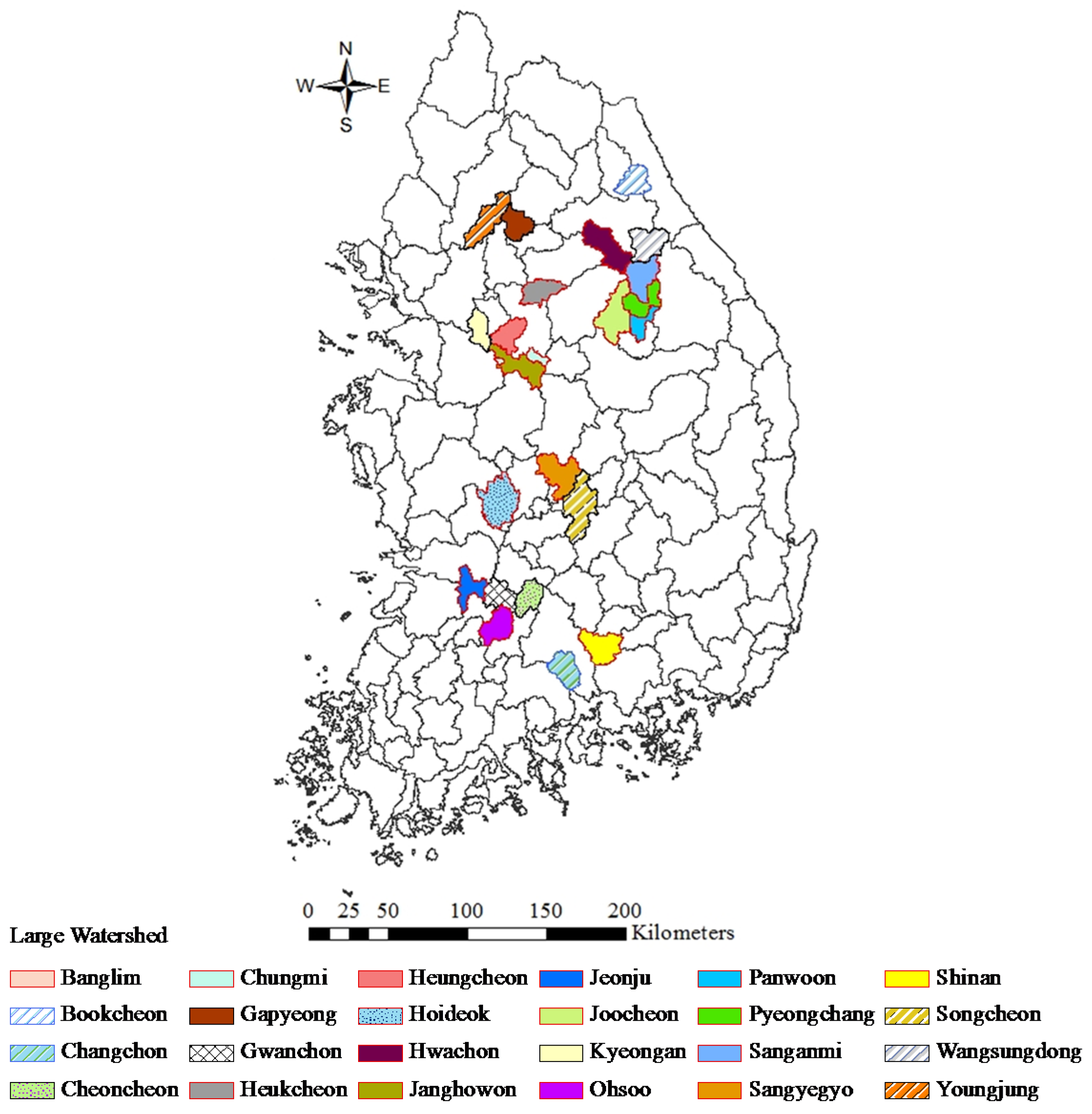
2.1. Study Area and Data

| WS ID | Watershed Name | Major Land Cover Distribution (km2) | Area | NOE | ME | α | CN | |||
|---|---|---|---|---|---|---|---|---|---|---|
| Forests | Agriculture | Urbanized | Grass | (km2) | (m) | (%) | ||||
| Small watersheds, Area ≤ 250 km2 | ||||||||||
| WS01 | Cheonwang | 97.05 | 57.51 | 30.82 | 3.86 | 42.32 | 29 | 26 | 13.40 | 66 |
| WS02 | Daeri | 47.31 | 1.67 | 0.39 | 0.25 | 60.45 | 39 | 424 | 48.13 | 75 |
| WS03 | Janggi | 36.76 | 23.80 | 2.44 | 1.11 | 62.80 | 42 | 146 | 21.50 | 70 |
| WS04 | Dopyeong | 106.03 | 27.75 | 15.42 | 3.70 | 138.36 | 34 | 173 | 28.71 | 64 |
| WS05 | Chunyang | 105.06 | 23.66 | 2.69 | 5.20 | 143.10 | 40 | 197 | 34.30 | 60 |
| WS06 | Cheongju | 14.95 | 14.48 | 17.23 | 0.50 | 161.44 | 70 | 202 | 20.10 | 69 |
| WS07 | Boksu | 119.09 | 30.83 | 5.02 | 1.30 | 161.90 | 26 | 343 | 35.50 | 60 |
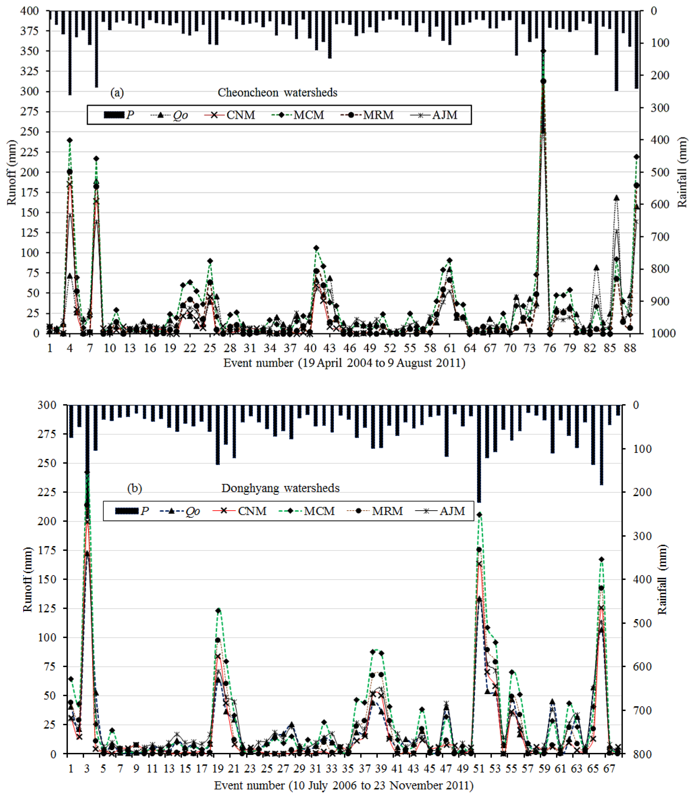
| WS08 | Donghyang | 111.34 | 44.76 | 4.51 | 2.67 | 164.66 | 68 | 911 | 35.09 | 64 |
| WS09 | Maeil | 152.06 | 20.79 | 0.48 | 0.13 | 174.86 | 60 | 517 | 39.65 | 53 |
| WS10 | Yulgeuk | 42.41 | 110.95 | 15.47 | 3.72 | 179.95 | 38 | 113 | 7.50 | 71 |
| WS11 | Toigyewon | 137.55 | 37.86 | 14.06 | 6.05 | 200.45 | 44 | 285 | 26.70 | 64 |
| WS12 | Jungrang | 94.17 | 15.54 | 83.26 | 2.01 | 208.41 | 42 | 219 | 17.30 | 67 |
| WS13 | Soochon | 79.46 | 108.11 | 18.42 | 2.09 | 223.19 | 31 | 76 | 15.40 | 73 |
| WS14 | Guryong | 163.71 | 65.18 | 7.08 | 3.95 | 245.50 | 33 | 244 | 26.60 | 65 |
| WS15 | Yoosung | 167.64 | 48.15 | 17.64 | 7.29 | 249.63 | 65 | 349 | 27.30 | 71 |
| Large watersheds, Area > 250 km2 | ||||||||||
| WS01 | Kyeongan | 153.70 | 44.73 | 37.15 | 11.50 | 256.91 | 89 | 165 | 22.86 | 63 |
| WS02 | Jeonju | 169.78 | 59.36 | 39.36 | 5.03 | 278.00 | 72 | 168 | 28.33 | 70 |
| WS03 | Cheoncheon | 183.91 | 72.31 | 8.18 | 16.85 | 284.03 | 89 | 554 | 32.23 | 58 |
| WS04 | Gwanchon | 217.56 | 62.11 | 7.90 | 7.65 | 301.26 | 49 | 420 | 33.70 | 70 |
| WS05 | Gapyeong | 274.05 | 18.52 | 5.28 | 2.21 | 305.12 | 39 | 490 | 45.40 | 69 |
| WS06 | Heukcheon | 232.82 | 57.19 | 13.04 | 3.75 | 307.82 | 19 | 253 | 32.70 | 59 |
| WS07 | Heungcheon | 124.45 | 135.52 | 31.07 | 7.32 | 309.08 | 28 | 112 | 13.80 | 67 |
| WS08 | Bookcheon | 377.04 | 123.35 | 36.04 | 15.97 | 330.20 | 38 | 733 | 53.53 | 52 |
| WS09 | Changchon | 280.95 | 35.50 | 5.64 | 2.45 | 335.07 | 83 | 523 | 41.82 | 68 |
| WS10 | Ohsoo | 210.60 | 118.95 | 11.00 | 3.92 | 350.09 | 61 | 243 | 24.60 | 62 |
| WS11 | Wangsungdong | 374.02 | 20.97 | 1.33 | 2.12 | 378.67 | 24 | 866 | 47.80 | 61 |
| WS12 | Sanganmi | 350.57 | 40.55 | 4.31 | 2.62 | 402.45 | 26 | 778 | 39.40 | 61 |
| WS13 | Shinan | 301.16 | 87.52 | 9.36 | 3.32 | 411.96 | 56 | 244 | 31.25 | 71 |
| WS14 | Janghowon | 181.36 | 182.02 | 23.52 | 10.92 | 431.23 | 26 | 678 | 16.80 | 65 |
| WS15 | Youngjung | 288.93 | 101.36 | 30.87 | 12.28 | 445.36 | 29 | 268 | 27.00 | 61 |
| WS16 | Sangyegyo | 331.21 | 134.62 | 13.42 | 3.29 | 496.30 | 35 | 268 | 29.40 | 71 |
| WS17 | Cheongmi | 215.69 | 219.85 | 29.82 | 14.12 | 514.66 | 30 | 147 | 16.70 | 78 |
| WS18 | Hwachon | 443.38 | 50.85 | 6.45 | 0.91 | 523.20 | 59 | 499 | 41.40 | 57 |
| WS19 | Banglim | 448.67 | 56.84 | 5.81 | 3.30 | 527.12 | 30 | 763 | 40.20 | 63 |
| WS20 | Joocheon | 449.10 | 68.49 | 5.74 | 1.90 | 533.23 | 65 | 608 | 38.12 | 58 |
| WS21 | Hoideok | 362.89 | 105.74 | 94.04 | 23.68 | 609.15 | 41 | 170 | 25.70 | 70 |
| WS22 | Songcheon | 455.78 | 131.15 | 11.86 | 4.54 | 612.17 | 54 | 386 | 33.25 | 64 |
| WS23 | Pyeongchang | 609.60 | 79.87 | 8.92 | 4.47 | 697.67 | 64 | 734 | 40.30 | 64 |
| WS24 | Panwoon | 757.06 | 99.67 | 11.18 | 6.29 | 888.01 | 37 | 678 | 40.88 | 60 |
| Data Type | Parameter/Model | Statistics | |||||||
|---|---|---|---|---|---|---|---|---|---|
| Min | Mean | Median | Max | SD | Skewness | 25th Percentile | 75th Percentile | ||
| Observed data | P (mm) | 25.12 | 78.94 | 58.32 | 519.68 | 60.89 | 2.32 | 40.03 | 94.02 |
| P5 (mm) | 0.00 | 58.18 | 34.80 | 629.80 | 75.12 | 2.63 | 6.95 | 79.00 | |
| T (h) | 1.50 | 19.62 | 16.00 | 154.00 | 13.96 | 2.71 | 11.00 | 24.00 | |
| Qo (mm) | 0.17 | 37.26 | 19.36 | 364.38 | 46.81 | 2.46 | 8.10 | 46.96 | |
| Modeled data (Qc(mm)) | CNM | 0.00 | 24.36 | 6.22 | 415.63 | 44.50 | 3.50 | 1.49 | 24.48 |
| MCM | 0.56 | 44.56 | 26.08 | 487.31 | 55.02 | 2.63 | 7.71 | 56.38 | |
| MRM | 0.00 | 30.84 | 11.42 | 432.04 | 48.60 | 3.01 | 1.17 | 37.64 | |
| AJM | 1.62 | 34.69 | 20.05 | 375.63 | 41.52 | 2.97 | 9.95 | 40.47 | |

2.2. Development of a New Hydrological Model
2.2.1. The Traditional CN Model (CNM)
2.2.2. Mishra et al. Model (MRM)
2.2.3. Michel et al. Model (MCM)
2.2.4. The Proposed Model (AJM)
| Model ID | λ | CN | Model Expression | Remarks |
|---|---|---|---|---|
| CNM | 0.20 | NEH-4 Tables | Equations (1) and (2) | Original CN model in [17] |
| MCM | -do- | -do- | Equations (2), (5), (6) and (7) | Modification in [11] |
| MRM | -do- | -do- | Equations (2)–(4) | Modification in [1] |
| AJM | -do- | -do- | Equations (2) and (22) | Proposed Model |
3. Models’ Goodness-of-Fit Evaluation
4. Results and Discussion


| According to [35] | |||||
| Model | Performance Index Range | 0.75 < NSE ≤ 1.00 | 0.65 < NSE ≤ 0.75 | 0.50 < NSE ≤ 0.65 | NSE ≤ 0.50 |
| Performance Rating | Very good | Good | Satisfactory | Unsatisfactory | |
| CNM | 14 | 2 | 12 | 11 | |
| MCM | 10 | 8 | 13 | 8 | |
| MRM | 15 | 8 | 12 | 4 | |
| AJM | 36 | 3 | 0 | 0 | |
| According to [36] | |||||
| Model | Performance index range | NSE ≥ 0.90 | 0.80 ≤ NSE < 0.90 | 0.65 ≤ NSE < 0.80 | NSE < 0.65 |
| Performance rating | Very good | Good | Satisfactory | Unsatisfactory | |
| CNM | 2 | 6 | 8 | 23 | |
| MCM | 1 | 3 | 14 | 21 | |
| MRM | 1 | 10 | 12 | 16 | |
| AJM | 13 | 17 | 9 | 0 | |
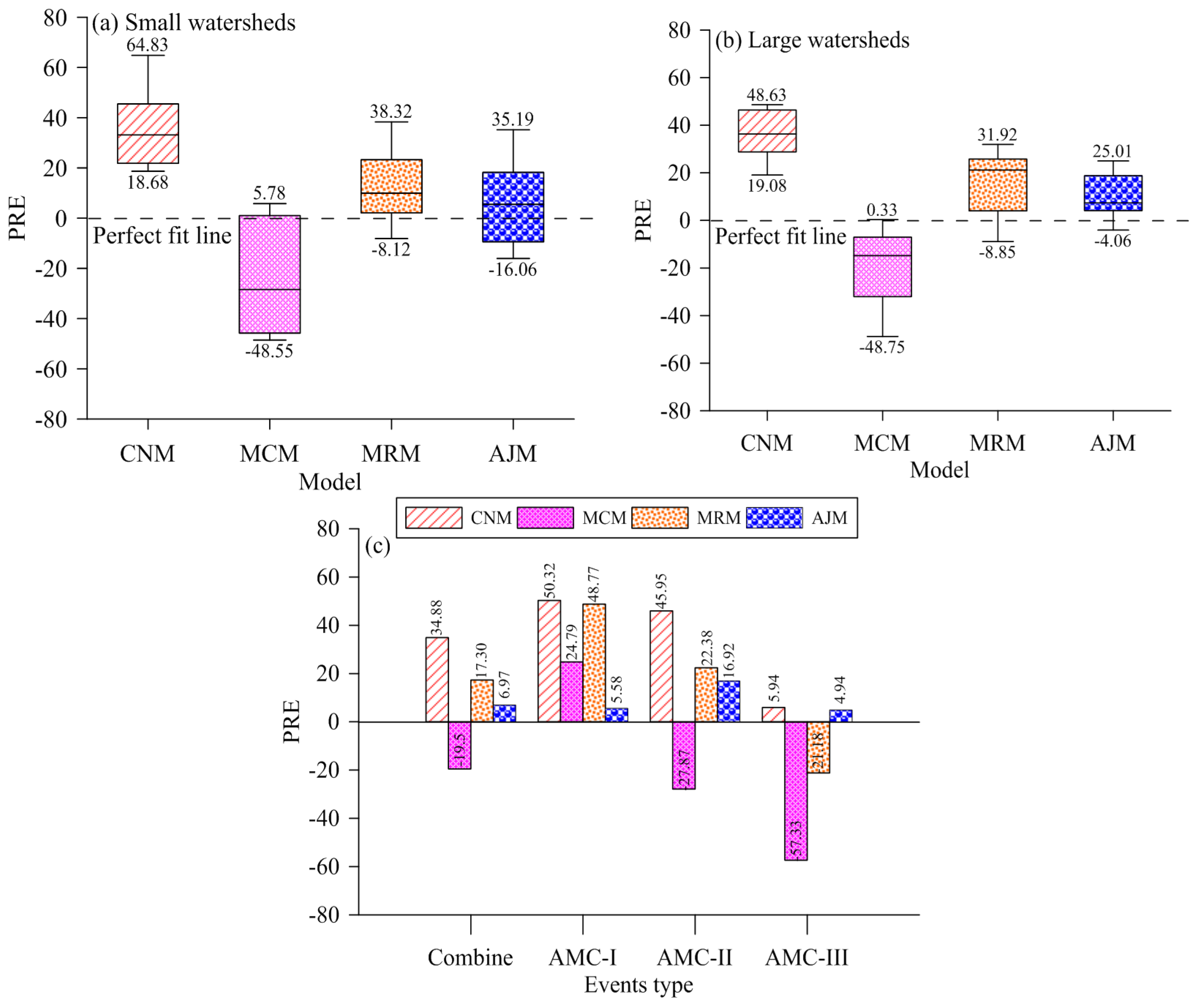
| According to [4,35] | |||||
| Model | Performance index range | PRE < 10 | 10 ≤ PRE < 15 | 15 ≤ PRE < 25 | PRE ≥ 25 |
| Performance rating | Very good | Good | Satisfactory | Unsatisfactory | |
| CNM | 1 | 0 | 10 | 28 | |
| MCM | 14 | 25 | 21 | 17 | |
| MRM | 14 | 2 | 13 | 10 | |
| AJM | 19 | 8 | 11 | 5 | |
| Test Type | ||||
|---|---|---|---|---|
| Data Type/Model | Kolmogorov-Smirnov | Anderson Darling | Chi-Squared | |
| Runoff | Best-fit distribution (Statistic) | |||
| Observed (Qo) | LP3 (0.023) | LP3 (1.273) | LP3 (21.821) | |
| Modeled (Qc) | CNM | PBW (0.033) | W (39.865) | PBW (30.628) |
| MCM | W (0.021) | LP3 (8.696) | GP (48.923) | |
| MRM | GEV (0.145) | W (37.654) | W (89.477) | |
| AJM | LP3 (0.024) | LP3 (1.523) | LP3 (15.949) | |


5. Conclusions
Acknowledgments
Author Contributions
Conflicts of Interest
References
- Mishra, S.K.; Sahu, R.K.; Eldho, T.I.; Jain, M.K. An improved Ia-S relation incorporating antecedent moisture in SCS-CN methodology. Water Resour. Manag. 2006, 20, 643–660. [Google Scholar] [CrossRef]
- Chung, W.H.; Wang, I.T.; Wang, R.Y. Theory-based SCS-CN method and its applications. J. Hydrol. Eng. 2010, 15, 1045–1058. [Google Scholar] [CrossRef]
- Garen, D.C.; Moore, D.S. Curve number hydrology in water quality modeling: Uses, abuses, and future directions. J. Am. Water Resour. Assoc. 2005, 41, 377–388. [Google Scholar] [CrossRef]
- Durbude, D.G.; Jain, M.K.; Mishra, S.K. Long-term hydrologic simulation using SCS-CN-based improved soil moisture accounting procedure. Hydrol. Process. 2011, 25, 561–579. [Google Scholar] [CrossRef]
- Grimaldi, S.; Petroselli, A.; Romano, N. Green-Ampt curve number mixed procedure as an empirical tool for rainfall-runoff modelling in small and ungauged basins. Hydrol. Process. 2013, 27, 1253–1264. [Google Scholar] [CrossRef]
- Patil, J.P.; Sarangi, A.; Singh, A.K.; Ahmad, T. Evaluation of modified CN methods for watershed runoff estimation using a GIS-based interface. Biosyst. Eng. 2008, 100, 137–146. [Google Scholar] [CrossRef]
- Wang, X.; Liu, T.; Yang, W. Development of a robust runoff-prediction model by fusing the rational equation and a modified SCS-CN method. Hydrol. Sci. J. 2012, 57, 1118–1140. [Google Scholar] [CrossRef]
- Garg, V.; Nikam, B.R.; Thakur, P.K.; Aggarwal, S.P. Assessment of the effect of slope on runoff potential of a watershed using NRCS-CN method. Int. J. Hydrol. Sci. Technol. 2013, 3, 141–159. [Google Scholar] [CrossRef]
- Ponce, V.M.; Hawkins, R.H. Runoff curve number: Has it reached maturity? J. Hydrol. Eng. 1996, 1, 11–19. [Google Scholar] [CrossRef]
- Schneider, L.E.; McCuen, R.H. Statistical guidelines for curve number generation. J. Irrig. Drain. Eng. 2005, 131, 282–290. [Google Scholar] [CrossRef]
- Michel, C.; Andréassian, V.; Perrin, C. Soil conservation service curve number method: How to mend a wrong soil moisture accounting procedure. Water Resour. Res. 2005, 41, 1–6. [Google Scholar] [CrossRef]
- Sahu, R.K.; Mishra, S.K.; Eldho, T.I.; Jain, M.K. An advanced soil moisture accounting procedure for SCS curve number method. Hydrol. Process. 2007, 21, 2872–2881. [Google Scholar] [CrossRef]
- Massari, C.; Brocca, L.; Barbetta, S.; Papathanasiou, C.; Mimikou, M.; Moramarco, T. Using globally available soil moisture indicators for flood modelling in Mediterranean catchments. Hydrol. Earth Syst. Sci. 2014, 18, 839–853. [Google Scholar] [CrossRef]
- Ajmal, M.; Kim, T.-W. Quantifying excess stormwater using SCS-CN-based rainfall runoff models and different curve number determination methods. J. Irrig. Drain. Eng. 2015, 141, 04014058. [Google Scholar] [CrossRef]
- Deshmukh, D.S.; Chaube, U.C.; Hailu, A.E.; Gudeta, D.A.; Kassa, M.T. Estimation and comparison of curve numbers based on dynamic land use land cover change, observed rainfall-runoff data and land slope. J. Hydrol. 2013, 492, 89–101. [Google Scholar] [CrossRef]
- Hawkins, R.H.; Ward, T.J.; Woodward, D.E.; van Mullem, J.A. Curve Number Hydrology-State of Practice; The American Society of Civil Engineers (ASCE): Reston, VA, USA, 2009. [Google Scholar]
- Natural Resources Conservation Service. Chapter 10: Hydrology. In National Engineering Handbook, Supplement A, Section 4; The United States Department of Agriculture: Washington, DC, USA, 2004. [Google Scholar]
- Seibert, J. On the need for benchmarks in hydrological modelling. Hydrol. Process. 2001, 15, 1063–1064. [Google Scholar] [CrossRef]
- Tramblay, Y.; Bouaicha, R.; Brocca, L.; Dorigo, W.; Bouvier, C.; Camici, S.; Servat, E. Estimation of antecedent wetness conditions for flood modelling in northern Morocco. Hydrol. Earth Syst. Sci. 2001, 16, 75–86. [Google Scholar]
- Woodward, D.E.; Hawkins, R.H.; Jiang, R.; Hjelmfelt, A.T., Jr.; van Mullem, J.A.; Quan, D.Q. Runoff curve number method: Examination of the initial abstraction ratio. In Proceedings of the World Water and Environmental Resources Congress, Philadelphia, PA, USA, 23–26 June 2003.
- Baltas, E.A.; Dervos, N.A.; Mimikou, M.A. Technical Note: Determination of the SCS initial abstraction ratio in an experimental watershed in Greece. Hydrol. Earth Syst. Sci. 2007, 11, 1825–1829. [Google Scholar] [CrossRef]
- D’Asaro, F.; Grillone, G. Empirical investigation of curve number method parameters in the Mediterranean area. J. Hydrol. Eng. 2012, 17, 1141–1152. [Google Scholar] [CrossRef]
- Perrin, C.; Michel, C.; Andréassian, V. Improvement of a parsimonious model for streamflow simulation. J. Hydrol. 2003, 279, 275–289. [Google Scholar] [CrossRef]
- Yuan, Y.; Nie, W.; McCutcheon, S.C.; Taguas, E.V. Initial abstraction and curve numbers for semiarid watersheds in southeastern Arizona. Hydrol. Process. 2014, 28, 774–783. [Google Scholar] [CrossRef]
- Yuan, Y.; Mitchell, J.K.; Hirschi, M.C.; Cooke, R.A.C. Modified SCS curve number method for predicting subsurface drainage flow. Trans. Am. Soc. Agric. Eng. 2001, 44, 1673–1682. [Google Scholar] [CrossRef]
- Brocca, L.; Melone, F.; Moramarco, T.; Singh, V.P. Assimilation of observed soil moisture data in storm rainfall-runoff modeling. J. Hydrol. Eng. 2009, 14, 153–165. [Google Scholar] [CrossRef]
- Tramblay, Y.; Bouvier, C.; Martin, C.; Didon-Lescot, J.F.; Todorovik, D.; Domergue, J.M. Assessment of initial soil moisture conditions for event-based rainfall-runoff modelling. J. Hydrol. 2010, 387, 176–187. [Google Scholar] [CrossRef]
- Beck, H.E.; de Jeu, R.A.M.; Schellekens, J.; van Dijk, A.I.J.M.; Bruijnzeel, L.A. Improving curve number based storm runoff estimates using soil moisture proxies. IEEE J. Sel. Top. Appl. Earth Obs. Remote Sens. 2009, 2, 250–259. [Google Scholar] [CrossRef]
- Massari, L.; Brocca, L.; Moramarco, T.; Tramblay, Y.; Lescot, J.-F.D. Potential of soil moisture observations in flood modelling: Estimating initial conditions and correcting rainfall. Adv. Water Res. 2014, 74, 44–53. [Google Scholar] [CrossRef]
- Harmel, R.D.; Smith, P.K.; Migliaccio, K.W.; Chaubey, I.; Douglas-Mankin, K.R.; Benham, B.; Shukla, S.; Muñoz-Carpena, R.; Robson, B.J. Evaluating, interpreting, and communicating performance of hydrologic/water quality models considering intended use: A review and recommendations. Environ. Model. Softw. 2014, 57, 40–51. [Google Scholar] [CrossRef]
- Legates, D.R.; McCabe, G.J., Jr. Evaluating the use of “goodness-of-fit” measures in hydrologic and hydroclimatic model validation. Water Resour. Res. 1999, 35, 233–241. [Google Scholar] [CrossRef]
- Chen, X.Y.; Chau, K.W.; Busari, A.O. A comparative study of population-based optimization algorithms for downstream river flow forecasting by a hybrid neural network model. Eng. Appl. Artif. Intell. 2015, 46, 258–268. [Google Scholar] [CrossRef]
- Wu, C.L.; Chau, K.W.; Li, Y.S. Methods to improve neural network performance in daily flows prediction. J. Hydrol. 2009, 372, 80–93. [Google Scholar] [CrossRef]
- Nash, J.; Sutcliffe, J. River flow forecasting through conceptual models part I-A discussion of principles. J. Hydrol. 1970, 10, 282–290. [Google Scholar] [CrossRef]
- Moriasi, D.N.; Arnold, J.G.; van Liew, M.W.; Binger, R.L.; Harmel, R.D.; Veith, T. Model evaluation guidelines for systematic quantification of accuracy in watershed simulations. Trans. Am. Soc. Agric. Biosyst. Eng. 2013, 50, 885–900. [Google Scholar]
- Ritter, A.; Muñoz-Carpena, R. Performance evaluation of hydrological models: Statistical significance for reducing subjectivity in goodness-of-fit assessments. J. Hydrol. 2013, 480, 33–45. [Google Scholar] [CrossRef]
- EasyFit Professional (Version 5.5). Mathwave Technologies, 2004–2010. Available online: www.mathwave.com (accessed on 15 July 2015).
© 2016 by the authors; licensee MDPI, Basel, Switzerland. This article is an open access article distributed under the terms and conditions of the Creative Commons by Attribution (CC-BY) license (http://creativecommons.org/licenses/by/4.0/).
Share and Cite
Ajmal, M.; Khan, T.A.; Kim, T.-W. A CN-Based Ensembled Hydrological Model for Enhanced Watershed Runoff Prediction. Water 2016, 8, 20. https://doi.org/10.3390/w8010020
Ajmal M, Khan TA, Kim T-W. A CN-Based Ensembled Hydrological Model for Enhanced Watershed Runoff Prediction. Water. 2016; 8(1):20. https://doi.org/10.3390/w8010020
Chicago/Turabian StyleAjmal, Muhammad, Taj Ali Khan, and Tae-Woong Kim. 2016. "A CN-Based Ensembled Hydrological Model for Enhanced Watershed Runoff Prediction" Water 8, no. 1: 20. https://doi.org/10.3390/w8010020