Case Study: A Real-Time Flood Forecasting System with Predictive Uncertainty Estimation for the Godavari River, India

Abstract

This work presents the application of the multi-temporal approach of the Model Conditional Processor (MCP-MT) for predictive uncertainty (PU) estimation in the Godavari River basin, India. MCP-MT is developed for making probabilistic Bayesian decision. It is the most appropriate approach if the uncertainty of future outcomes is to be considered. It yields the best predictive density of future events and allows determining the probability that a critical warning threshold may be exceeded within a given forecast time. In Bayesian decision-making, the predictive density represents the best available knowledge on a future event to address a rational decision-making process. MCP-MT has already been tested for case studies selected in Italian river basins, showing evidence of improvement of the effectiveness of operative real-time flood forecasting systems. The application of MCP-MT for two river reaches selected in the Godavari River basin, India, is here presented and discussed by considering the stage forecasts provided by a deterministic model, STAFOM-RCM, and hourly dataset based on seven monsoon seasons in the period 2001–2010. The results show that the PU estimate is useful for finding the exceedance probability for a given hydrometric threshold as function of the forecast time up to 24 h, demonstrating the potential usefulness for supporting real-time decision-making. Moreover, the expected value provided by MCP-MT yields better results than the deterministic model predictions, with higher Nash–Sutcliffe coefficients and lower error on stage forecasts, both in term of mean error and standard deviation and root mean square error.

1. Introduction

The severe effects of flooding events are usually mitigated through structural measures, such as river banks, flood dykes and dams, that reduce but do not eliminate the risk. Therefore, in many cases, it is necessary to develop complementary non-structural measures, mainly real-time Flood Forecasting and Warning Systems (FFWSs), in order to be able to improve the population resilience to natural hazards [1].

The forecasting models are fundamental components of the FFWSs and provide river stage/discharge predictions at sections of particular interest with forecast horizons appropriate to support the decision-makers activities, addressed to flood effect mitigation. However, these models only provide a deterministic forecast for the future event and do not deal with the decision-maker uncertainty on decisions.

Flood forecasting has been typically approached through rainfall-runoff and/or flood routing models. The former predict the discharge at selected river sections with a lead-time depending on the watershed time of concentration; the latter provide forecasts at downstream ends of river reaches with a lead-time limited by the wave travel time. Whatever the used model, many errors influence the forecast, making the assessment of the uncertainty of predictions fundamental to properly support the decision-makers’ activities [2,3,4,5,6,7,8,9,10]. Many studies are available in the literature on generating probabilistic forecasting from deterministic forecast by modeling the uncertainty in the single-valued hydrologic forecast [11,12,13]. These approaches address forecasting in terms of a single value plus uncertainty. Alternatively, the introduction of the Hydrological Uncertainty Processor [14,15] created the basis for the estimation of the flood predictive uncertainty, PU, which represents our best knowledge of the future outcomes. Specifically, the PU represents the probability of occurrence of a future value of a predictant conditional on all the information that can be obtained on the future value, usually provided by forecasting models [14,16].

Different processors for PU assessment have been introduced starting from Krzysztofowicz [14] who created the basis for PU estimation by introducing the Bayesian Forecasting System (BFS). Several other approaches to predictive uncertainty assessment were developed [4,17,18] which aim at assessing the mean and variance conditional on forecasts from several models. Todini [19] proposed the Model Conditional Processor (MCP) for estimating the PU. MCP allows the analytical treatment of the multivariate probability densities after converting both observations and model(s) predictions into the Normal space, as suggested by Krzysztofowicz [14]. Afterward, MCP was extended to the multi-model approach by Coccia and Todini [16] allowing a decision based on “multiple forecasts” provided by different deterministic models at the same time. The use of outputs from more than one model can significantly improve conditional forecasts of discharges or water stages, provided the models are structurally different as demonstrated by means of a systematic uncertainty analysis by Plate and Shahzad [20].

Moreover, Coccia [21] introduced the multi-temporal approach of MCP that answers questions such as “Which is the probability that the threshold will be exceeded within the next 24 h?” by considering several forecast time steps provided by the available forecasting models at the same time and including all of them into the Bayesian formulation. The multi-temporal approach of MCP (MCP-MT) has been tested on case studies selected in Italy by verifying if it could have represented a useful support for improving the effectiveness of forecast models already operational within the local FFWS. The analysis showed that the MCP-MT is potentially useful for supporting real-time decision-making mainly because it can provide information on the hydrometric thresholds exceedance probability within the time forecast horizon.

The present paper applies the MCP-MT to a study area, whose properties are very different from those of the case studies already analyzed mainly characterized by Mediterranean climate condition, steep river bed slope and small-medium drainage areas. Specifically, this work analyzes two reaches of the Godavari River, in India, that is affected by severe flooding problems during the monsoon season and flood forecasting issue is of great importance in this area. The selected case study is characterized by a very large drainage area and gentle river bed slope (≅0.3‰). Embankments have been constructed to prevent the flooding of deltaic areas, however considerably long reaches of the river upstream of the delta are vulnerable to floods. Scientific flood forecasting and advance warning have been found to be extremely beneficial to reduce the flood damages in these reaches. Flood forecasting activity started in 1974 with the opening of a Division office of Central Water Commission, but it is essentially based on real-time observations of the monitoring network and deterministic forecasts. This paper shows that in areas located in developing countries significant additional benefits for the FFWS could be obtained, if the MCP-MT is used to estimate the predictive uncertainty of the forecasts. STAFOM-RCM is used as basic forecast model [22].

The paper is organized as follows: Section 2 summarizes the main characteristics of the multi-temporal approach of MCP. Section 3 is dedicated to a brief overview of the forecasting model STAFOM-RCM. Section 4 contains the description of the selected case study and dataset. Section 5 presents the analysis of the results obtained through the application of the multi-temporal approach of MCP, based on performance evaluation measures clearly defined. Section 6 outlines final remarks on the potential usefulness of the approach in the selected study area.

2. Predictive Uncertainty Assessment: The Model Conditional Processor in the Multi-Temporal Approach

The main characteristics of the multi-temporal approach of the Model Conditional Processor, MCP-MT, used in this study for predictive uncertainty estimate are outlined in what follows. For additional details, the reader can refer to Coccia [21] and Coccia and Todini [16].

MCP was first derived in single-temporal approach [16] and is essentially based on the definition of the multi-variate conditional distribution, i.e., the density of the predictant conditional model predictions by considering a unique forecast horizon. This is obtained by dividing the joint predictand-prediction distribution, a multi-normal in the homoscedastic case or a multi-truncated-normal in the heteroscedastic case, by the joint marginal distribution of the predictor(s) [16]. These distributions are estimated by simulating forecasts, through the application of any forecasting model, for an identified calibration data period. Specifically, the calibration consists in identifying the joint and marginal probability distributions required for Bayes theorem application.

Since multivariate joint distributions can be formulated and effectively analytically treated in a very limited number of cases, Krzysztofowicz [14] suggested transforming the observations and model forecasts into a Gaussian or normal space via a non-parametric transformation based on the Normal Quantile Transform (NQT) [23,24,25]. The MCP application is based on four steps depicted in Figure 1.

• First, the observations, $y$, and the forecasts, ${\widehat{y}}_k$ (k = 1, …, M, M = number of available forecasts provided by M different forecasting models), are converted into the normal space using the NQT (Figure 1, blue box on the left side). The original variables, $y$ and ${\widehat{y}}_k$, whose empirical cumulative distribution functions are computed using the Weibull plotting position (see Equations (1) and (2)), are converted to their transformed values $\eta$ and ${\widehat{\eta }}_k$, respectively, which are normally distributed with zero mean and unit variance. According to the NQT definition, the probability of each element of $\eta$ and ${\widehat{\eta }}_k$ is the same as its original corresponding value in $y$ and ${\widehat{y}}_k$. Thus, the relation between the original variables and their transformed values is:

  $$P(y<y_i)=\frac{i}{n+1}=P(\eta <{\eta }_i)$$

  (1)

  $$P({\widehat{y}}_k<{\widehat{y}}_{ki})=\frac{i}{n+1}=P({\widehat{\eta }}_k<{\widehat{\eta }}_{ki})$$

  (2)

  with i = 1, …, n, n is the number of the historical available data, and i is the plotting position order.
• In the normal space, the joint probability distribution of observed and predicted variables, $f(\eta ,{\widehat{\eta }}_k)$, is assumed to be a Normal Multivariate Distribution in the first formulation [19] (Figure 1, red box on the left side) or composed by two Truncated Normal Multivariate Distributions as proposed by Coccia and Todini [16].
• The predictive density is obtained applying the Bayes Theorem (Figure 1, green box on the right side):

  $$f(\eta |{\widehat{\eta }}_k)=\frac{f(\eta ,{\widehat{\eta }}_1,.......,{\widehat{\eta }}_M)}{f({\widehat{\eta }}_1,.......,{\widehat{\eta }}_M)}$$

  (3)
  It is normally distributed with mean, $\mu (\eta |{\widehat{\eta }}_k)$, and variance, ${\sigma }^2(\eta |{\widehat{\eta }}_k)$, defined as:

  $$\mu (\eta |{\widehat{\eta }}_k)={\Sigma }_{\eta \widehat{\eta }}\cdot {{\Sigma }_{\eta \widehat{\eta }}}^{-1}\cdot \left[\begin{array}{l}{\widehat{\eta }}_1\\ .\\ .\\ {\widehat{\eta }}_M\end{array}\right]$$

  (4)

  $${\sigma }^2(\eta |\widehat{\eta })=1-{\Sigma }_{\eta \widehat{\eta }}\cdot {{\Sigma }_{\eta \widehat{\eta }}}^{-1}\cdot {{\Sigma }_{\eta \widehat{\eta }}}^T$$

  (5)
• The PU in the normal space is finally reconverted to the real space by applying the Inverse NQT (Figure 1, grey box on the right side).

The described approach can be computed for single or multi-model applications, i.e., M = 1 or M > 1, respectively, and also allows assessing the flooding probability, i.e., the probability to exceed established water levels, of fundament interest within FFWSs based on fixed hydrometric thresholds. The probability to exceed a threshold value, a, can be easily computed as the PU integral above the threshold value, ${\eta }_a$, in the normal space (Figure 1, left side):

$$P(y>a|\widehat{y}={\widehat{y}}^{*})={\displaystyle \underset{a}{\overset{\infty }{\int }}f(y|\widehat{y}={\widehat{y}}^{*})dy}={\displaystyle \underset{{\eta }_a}{\overset{\infty }{\int }}f(\eta |\widehat{\eta }={\widehat{\eta }}^{*})d\eta }$$

(6)

As mentioned above, the first MCP formulation [19] uses a single forecast horizon (single-temporal approach) and a unique data sample, while two Truncated Normal Distributions (TNDs) were introduced by Coccia and Todini [16] to distinguish between uncertainties for high and low flows. Specifically, the data are divided in two different samples, each supposed to belong to a different TND. The truncation threshold, splitting the whole dataset in two different samples, is identified over the predicted variable by minimizing the predictive variance for the upper sample, the one related to high flows.

The multi-temporal approach of MCP, named MCP-MT, is based on the same concepts but considers many forecasting horizons, i.e., lead-times, at the same time [21]. In detail, T forecast time steps are provided by the $M$ deterministic models of the early warning system and all of them are included into the Bayesian formulation [21]. The MCP-MT accounts for the time dependence of forecasting errors without the need of defining a specific error model and computes the errors independently for each forecast horizon, i.e., the forecast referring to a specific lead-time is compared with the corresponding observed value.

Specifically, the Normal Multivariate Space is composed by $T\times (M+1)$ variables, namely the observed values, ${\eta }_t$, t = 1, …, T, and the forecasts of the M models at each time step, ${\widehat{\eta }}_{t,k}$, k = 1, …, M, t = 1, …, T. Therefore, the predictive uncertainty in the normal space is a Normal Multivariate Distribution, composed by T variables, $f({\eta }_1,\dots ,{\eta }_T|{\widehat{\eta }}_{1,1},\dots ,{\widehat{\eta }}_{T,M})$, henceforth abbreviated as $f({\eta }_t|{\widehat{\eta }}_{t,k})$.

The joint distribution of observed and predicted variable is a normal $T\times (M+1)$-variate distribution with mean, ${\mu }_{{\eta }_t,{\widehat{\eta }}_t,k}$, and variance, ${\displaystyle {\sum }_{{\eta }_t,{\widehat{\eta }}_{t,k}}}$, equal to:

$${\mu }_{{\eta }_t,{\widehat{\eta }}_t,k}=\left[\begin{array}{c}0\\ ..\\ ..\\ 0\end{array}\right]$$

(7)

$${\displaystyle {\sum }_{{\eta }_{t,}{\widehat{\eta }}_{t,k}}=\left[\begin{array}{cc}{\Sigma }_{\eta \eta }& {\Sigma }_{\eta \widehat{\eta }}\\ {\Sigma }_{\eta \widehat{\eta }}^T& {\Sigma }_{\widehat{\eta }\widehat{\eta }}\end{array}\right]}$$

(8)

The PU can be expressed through a Bayesian combination as follows:

$$f({\eta }_t|{\widehat{\eta }}_{t,k})=\frac{f({\eta }_1,...,{\eta }_T,{\widehat{\eta }}_{1,1,}...,{\widehat{\eta }}_{T,M})}{f({\widehat{\eta }}_{1,1,}...,{\widehat{\eta }}_{T,M})}=\frac{f({\eta }_t,{\widehat{\eta }}_{t,k})}{f({\widehat{\eta }}_{t,k})}$$

(9)

By solving Equation (9), the PU is estimated through the normal distribution:

$$f({\eta }_t|{\widehat{\eta }}_{t,k}={\widehat{\eta }}_{t,k}^{*})=N\left({\mu }_{{\eta }_t|{\widehat{\eta }}_{t,k}={\widehat{\eta }}_{t,k}^{*}},{\Sigma }_{{\eta }_t|{\widehat{\eta }}_{t,k}={\widehat{\eta }}_{t,k}^{*}}\right)$$

(10)

where ${\widehat{\eta }}_{t,k}^{*}$ represents a realization of ${\widehat{\eta }}_{t,k}$.

The PU represented by Equation (10) describes the joint predictive distribution of the observed values for the different T predicted time steps, i.e., lead-times. This predictive distribution gives fundamental information such as the flooding probability within the time horizon T* (where 1 ≤ T* ≤ T) that can be computed using Equation (11), complementary to 1 of the integrative of the PU below the value of the threshold level:

$$P_{T^{*}}(max\left[{\eta }_t\right]>{\eta }_D|{\widehat{\eta }}_{i,k}={\widehat{\eta }}_{i,k}^{*})=1-{\displaystyle \underset{-\infty }{\overset{{\eta }_D}{\int }}....}{\displaystyle \underset{-\infty }{\overset{{\eta }_D}{\int }}f({\eta }_i|}{\widehat{\eta }}_{i,k}={\widehat{\eta }}_{i,k}^{*})d{\eta }_1\dots d{\eta }_t$$

(11)

where t = 1, …, T* and ${\eta }_D$ is the transformed of the threshold level in the Normal Space. This probability takes into account the fact that the flooding water level may be exceeded in any one of the considered time steps.

MCP-MT application requires as input the observed stage values and the ones forecasted by the deterministic model/models with different T lead-times and provides as output the density of the predictand conditional on the deterministic predictions. For each lead-time and for each time step MCP-MT provides as output the expected value of the identified multi-variate conditional distribution, the cumulated 0.05 probability quantiles (5%, 10%, …, 95%) and the probability of hydrometric thresholds exceedance within the considered lead-time.

3. Forecasting Model: STAFOM-RCM

For sake of completeness, the main characteristics of the forecasting model used in the study are briefly described in what follows. For additional details, the reader can refer to Barbetta et al. [22,26].

The real-time flood routing model named STAFOM-RCM (STAge FOrecasting Model-Rating Curve Model) provides future stage predictions by explicitly estimating at each time of forecast, $t_f$, the lateral inflow along the selected river reach [22]. STAFOM-RCM is based on two models coupled in such a way as to provide one forecast stage value at each time step. Specifically:

• STAFOM provides a first estimate of the forecast stage (preliminary forecast) at the downstream end, $h_d^{\prime }$, computed as:

  $$h_d^{\prime }\left(t_f+\Delta t^{*}\right)={\left\{\frac{1}{\lambda }\left[C_1^{*}\left(Q_u\left(t_f\right)+q_{for}\left(t_f\right)L\right)+C_2^{*}{\left(h_d\left(t_f\right)\right)}^{\delta }\right]\right\}}^{1/\delta }$$

  (12)

  where $h_d\left(t_f\right)$ is the stage observed at the downstream end at $t_f$, $\Delta t^{*}$ is the forecast lead-time (typically assumed equal to the mean observed wave travel time, T_L, of the reach), $Q_u\left(t_f\right)$ is the observed upstream discharge at $t_f$, L is the river reach length, and $\lambda$ and $\delta$ are parameters of the downstream rating curve ($Q_d=\lambda h_d^{\delta }$). $C_1^{*}$ and $C_2^{*}$ refer to the Muskingum parameters K and θ respecting the constraint $\Delta t^{*}=2K\theta$:

  $$C_1^{*}=\frac{K\theta +0.5\Delta t^{*}}{K-K\theta +0.5\Delta t^{*}};C_2^{*}=\frac{K-K\theta -0.5\Delta t^{*}}{K-K\theta +0.5\Delta t^{*}}$$

  (13)

  q_for is the lateral flow contribution for unit channel length estimated as [27]:

  $$q_{for}\left(t_f\right)=\frac{A_d\left(t_f\right)-A_u\left(t_f-T_L\right)}{T_L}$$

  (14)

  where $A_u$ and $A_d$ are the upstream and downstream flow areas, respectively, computed by using the relationship between the stage and the flow area estimated from the knowledge of the section geometry; T_L is the flood wave travel time assumed equal to the lead-time, $\Delta t^{*}$, for forecasting purposes. The lateral flow is assumed uniformly distributed along the branch and, hence, the total lateral discharge entering in the reach in the time interval $(t_f;t_f+\Delta t^{*})$, $Q_l$, is equal to $q_{for}(t_f)L$.
• RCM, improves the preliminary forecast stage from STAFOM by exploiting the following relationship between the upstream and downstream discharge, $Q_d$, [27,28]:

  $$Q_d\left(t+T_L\right)=\alpha \frac{A_d\left(t+T_L\right)}{A_u\left(t\right)}{Q}_u\left(t\right)+\beta$$

  (15)

  where α and β are the RCM model parameters.

Specifically, the preliminary forecast stage, $h_d^{\prime }$, is considered for computing the downstream flow area, $A_d^{\prime }$, at time $\left(t_f+\Delta t^{*}\right)$ and, hence, the quantity $\frac{A_d^{\prime }\left(t_f+\Delta t^{*}\right)}{A_u\left(t_f\right)}{Q}_u\left(t_f\right)$. The refined forecast stage is finally derived as:

$${\widehat{h}}_d\left(t_f+\Delta t^{*}\right)={\left\{\frac{1}{\lambda }\left[\alpha \frac{A_d^{\prime }\left(t_f+\Delta t^{*}\right)}{A_u\left(t_f\right)}{Q}_u\left(t_f\right)+\beta \right]\right\}}^{1/\delta }$$

(16)

The model requires as input data only the stages at the two end sections along with accurate rating curves, necessary to estimate the upstream inflow and to derive the downstream parameters λ and δ, and topographic surveys of both sections for the computation of the flow area. Finally, the availability of past recorded flood events is required to estimate the mean wave travel time and the relative α and β parameters.

STAFOM-RCM was tested on different river reaches, mainly located in the Upper-Middle Tiber River basin, central Italy, providing mostly reliable estimates of future stage with lead-time from a few up to several hours.

4. Study Area, Model Setting and Dataset

The Godavari River basin subtended by the hydrometric section of Polavaram gauged section is selected as study area. The Godavari River is the largest of the peninsular rivers and third largest in India. It drains a total area of 312,812 km² that is about 10% of India’s total geographical area. The Godavari River rises at an elevation of 1067 m a.s.l. in the Western Ghats, near Thriambak Hills in the Nasik district of Maharashrta, and after flowing for about 1465 km, in a generally southeast direction, it falls into the Bay of Bengal (see Figure 2). The mean annual rainfall varies from 1000 to 3000 mm. The Godavari basin receives its maximum rainfall during the Southwest monsoon; specifically, 84% of the annual rainfall falls during the period starting in mid June and ending by mid October. The monsoon currents strike the West Coast of the peninsula from west and southwest, meet the Western Ghats or Sahyadri Range which present almost an uninterrupted barrier ranging from 600 to 2100 m a.s.l. Rainfall is governed largely by the orography of the area, which leads to variation in the amount of precipitation.

Since the mid 1960s, the Central Water Commission is conducting hydro-meteorological observations in the Godavari basin. Specifically, hydrometric observation stations have been established on main Godavari River as well as on all the important tributaries. The monitoring network consists in more than 60 gauged stations, the location of most of which is shown in Figure 2 where the three gauged river sites selected for the study are also highlighted (Perur, Bhadrachalam and Polavaram hydrometric stations).

The network of river gauge, discharge and rainfall stations transmit the data collected on real-time basis to the flood forecasting center in the Lower Godavari Division at Hyderabad, using high frequency wireless sets. The river stage is observed at every hour on all days from 15 June to 15 October. River discharge is observed once in a day.

The two Godavari River reaches bounded upstream by the gauged section of Perur (drainage area = 268,200 km²) and Bhadrachalam (drainage area = 280,505 km²), and downstream by the hydrometric site of Polavaram (drainage area = 307,800 km²) are selected for the application of the STAFOM-RCM model.

During the monsoon, the Godavari River overtops its banks, inundating certain flood prone areas. One of these is situated between the gauged sections of Perur, upstream, and Polavaram, downstream.

Perur-Polavaram is a 206 km long branch with a large intermediate drainage area of 39,600 km², which represents 13% of the entire catchment. It has a mean observed wave travel time between 20 and 24 h. The shorter investigated reach, Bhadrachalam-Polavaram, is 73 km long and is characterized by an intermediate drainage area that is about 9% of the downstream total one. The mean wave travel time of the reach is found equal to about 10–12 h. The mean section width of the Godavari River between the gauged site of Perur and Polavaram is about 1300 m. The main properties of the investigated river reaches are summarized in

Table 1. Godavari River: main properties of the selected river reaches (L, length; Aup and Adown, upstream and downstream drainage area; Aint, intermediate drainage area; S₀, mean bed slope; B, mean section width; T_L, mean wave travel time).

	River Reach	L (km)	Aup (km2)	Adown (km2)	Aint (km2)	S0	B (m)	TL (h)
reach 1	Bhadrachalam-Polavaram	73	280,505	307,800	27,295 (9%)	0.00025	1300	10–12
reach 2	Perur-Polavaram	206	268,200		39,600 (13%)	0.0003		20–24

, while the geometry of the Polavaram gauged section, where the stage forecast and the PU estimate are provided, is represented in Figure 3.

As concerns the parameter setting, while the model parameters λ = 13.7, δ = 3 and θ = 0.5 are constant for both river reaches and all the lead times, K = Δt*, α and β change depending on the lead-time.

Continuous hourly stage data are available for the monsoon season (June–October) for the period 2001–2010. However, data checking showed that for 2006, 2008 and 2009 years the data series are affected by a large number of missing or unreliable values for at least one of the stations and, for this reason, these years are not included in the used dataset that, definitely, consists of 19,294 and 17,339 hourly stage data for Perur-Polavaram and Bhadrachalam-Polavaram, respectively.

5. Results and Discussion

The proper objective of a forecast is to obtain the predictive density conditional on prior information and in particular on model forecasts. Nonetheless, it is worthwhile showing that the expected value of the predictand conditional on the model forecasts already improves over the original model future prediction and, for this reason, statistics of both, the original model forecasts and the expected conditional values, were also discussed and compared. The metrics used for evaluation are delineated in what follows.

5.1. Performance Evaluation Measures

The accuracy of the STAFOM-RCM model is quantified by considering the following performance criteria. The same verification metrics are used for comparing the MCP-MT performance, in terms of expected value, with that of the deterministic forecasting model STAFOM-RCM.

The imminence with which the forecast model reproduces the observed stages can be measured using the Nash–Sutcliffe efficiency coefficient [29], NS:

$$NS=\left[1-\frac{{\displaystyle \sum _{i=1}^N{\left(h_{obsi}-h_{fori}\right)}^2}}{{\displaystyle \sum _{i=1}^N{\left(h_{obsi}-{\overline{h}}_{obs}\right)}^2}}\right]$$

(17)

where h_obsi is the ith ordinate of the observed stage-hydrograph; ${\overline{h}}_{obs}$ is the mean of the observed stage-hydrograph ordinates; h_fori is the ith ordinate of the forecast stage-hydrograph; and N is the total number of stage-hydrograph ordinates to be forecasted.

NS equal to 1 identifies a perfect model efficiency, while an efficiency lower than zero indicates that the mean value of the observed time series would have been a better predictor than the model output.

The Root Mean Square Error (RMSE) in reproducing the observed stage hydrograph is also used and computed as:

$$RMSE=\sqrt{\frac{{\displaystyle \sum _{i=1}^N{\left(h_{obsi}-h_{fori}\right)}^2}}{N}}$$

(18)

Moreover, the mean, m, and the standard deviation, σ, of the absolute error on stage forecast, er_h, are used for evaluating the accuracy on stage hydrograph reproduction:

$$er\_h_i=\left|h_{fori}-h_{obsi}\right|i=1,.......,N$$

(19)

Finally, the accuracy of the forecast stage hydrograph is also assessed through the coefficient of persistence, PC, [30] which takes values smaller or equal to 1, this last corresponding to perfect performance. PC compares the forecasts with the prediction of the no-model, which assumes the steady state over the forecast lead-time:

$$PC=\left(1-\frac{{\displaystyle \sum _i{\left(h_{obsi}-h_{fori}\right)}^2}}{{\displaystyle \sum _i{\left(h_{obsi}-h_{obs(i-\Delta t^{*})}\right)}^2}}\right)$$

(20)

where Δt* is the lead-time and $h_{obs(i-\Delta t^{*})}$ is the (i − Δt*)th ordinate of the observed stage hydrograph. The closer PC to 1 (perfect forecast), the more accurate the model, while negative values indicates that the last observed stage would be a better future estimate than the model forecast.

5.2. Forecasting Model

STAFOM-RCM is run continuously in hindcast mode for the selected data periods (i.e., monsoon season for years 2001, 2002, 2003, 2004, 2005, 2007 and 2010) considering forecast lead-times from 1 h to 12 and 24 h, with an hourly time step, for the shorter reach (Bhadrachalam-Polavaram, identified as reach 1) and the longer branch (Perur-Polavaram, denominated as reach 2), respectively.

The performance of the deterministic forecasting model for the characteristic lead-times of the investigated reaches is summarized in

Table 2. Polavaram section (MCP-MT calibrated considering all the available dataset): mean (m) and standard deviation (σ) of the absolute error on stage forecast (er_h), Nash–Sutcliffe coefficient (NS), root mean square error (RMSE), and coefficient of persistence (PC), for the deterministic forecasting model, STAFOM-RCM, and the expected value estimated by the MCP-MT for the two investigated reaches.

River Reach	Lead-Time (h)	STAFOM-RCM					MCP-MT Expected Value
		er_h (m)		NS	RMSE (m)	PC	er_h (m)		NS	RMSE (m)	PC
		m	σ				m	σ
reach 1	10	0.196	0.223	0.989	0.297	0.56	0.117	0.159	0.995	0.198	0.81
	12	0.202	0.220	0.989	0.298	0.67	0.136	0.184	0.993	0.228	0.81
reach 2	20	0.344	0.403	0.960	0.530	0.34	0.283	0.328	0.973	0.433	0.56
	24	0.353	0.413	0.958	0.543	0.48	0.269	0.317	0.975	0.416	0.70

in terms of the selected evaluation metrics computed considering all the investigated time series of hourly data. Specifically, the results for 10 and 12 h lead-time are presented for reach 1, while longer forecast horizons, equal to 20 and 24 h, were considered for reach 2.

As it can be seen, STAFOM-RCM is found accurate for the selected lead-times with very high values of the NS coefficient, always higher than 0.95. We also note errors on stage forecast with mean values equal to about 0.2 m and 0.35 m for reach 1 and reach 2, respectively that can be considered low if compared with the mean observed stage during the used datasets equal to about 7 m with a standard deviation close to 2.7–2.8 m. In addition, the root mean square error indicates a satisfactory performance of the model, with values lower than 0.3 m for the shorter reach and slightly above 0.5 m for the longer branch. Finally, the PC values computed for the whole dataset suggest that the deterministic model forecasts would represent an added value for the real-time flood monitoring and management system providing more useful information than the no-model that is based the persistence assumption. By way of example, the performance of STAFOM-RCM for all the investigated lead-times is summarized in Figure 4 in terms of some selected evaluation metrics. As it can be seen, the results of the forecasting model can be considered satisfactory even for longer lead-times (see Table 2) being substantially unchanged in the range 8–12 h for reach 1. Therefore, considering the need for a trade-off between the forecast accuracy and the required forecast period, which should be long enough to allow the implementation of the first mitigation/management operations, in this study the forecast horizon of 10–12 h are deeply analyzed. Similar considerations can be done for reach 2 identifying, in this case, 20–24 h as optimal forecast horizon.

The results show that the STAFOM-RCM model outcomes could be conveniently used to support the current operational flood forecasting system in the Godavari River basin. Actually, the main contribution would be the predicative uncertainty estimate through the MCP-MT application as demonstrated in the following section.

5.3. Predictive Uncertainty Estimate Using MCP-MT

The multi-temporal MCP is applied considering the forecast stage provided by STAFOM-RCM for both the selected river reaches. Therefore, the single-model configuration for MCP-MT is considered with M, number of available forecast, equal to 1.

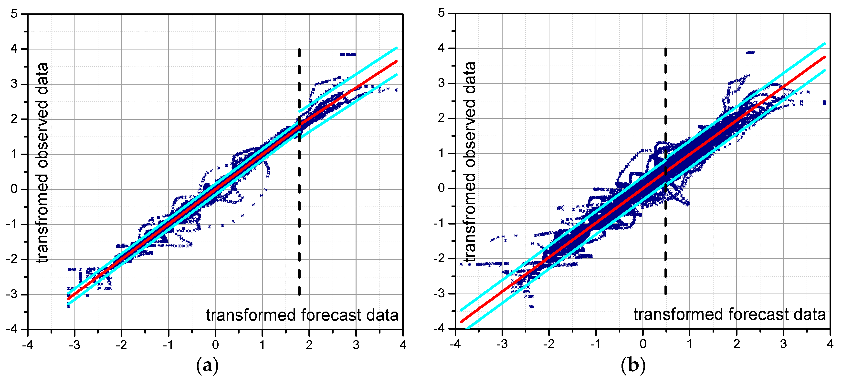
The first analysis is performed by using the complete dataset of simulated forecasts to calibrate MCP-MT, i.e., for identifying the joint and marginal probability distributions. Figure 5 shows the joint distributions identified in the normal space for the forecasting model considering a lead-time of 12 h and 24 h for reach 1 and reach 2, respectively. The threshold automatically identified by the MCP-MT in order to optimize the sample data division for representing low and high flows separately is also depicted in the figure. The transformed of the forecast stage threshold, η_tr, is equal to 1.79 when STAFOM-RCM is applied to reach 1 (Figure 5a), while a different value of 0.5 is identified for reach 2 (Figure 5b). Specifically, the threshold identified for reach 2 divides the data into two samples, the first corresponding to low flows that include 68% of the data and the second one referring to high flows and containing 32% of the entire sample.

It is worth noting that the data truncation for reach 1 (first sample referring to low-medium flows including 96% of data, second sample for high flows corresponding to 4% of the data) does not disagree with the hypothesis of homoscedasticity as the standard deviation of both samples is very similar. Moreover, it might be of interest to mention that a first study based on a different data sample spitting was attempted. Specifically, when dealing with flood forecasting four different states (peak flow, base flow and transitory states occurring during the rising and recession limbs) can be considered. To this end, the joint distribution can be assumed as composed by four TNDs. However, the first results seem to indicate that the MCP-MT performance is not significantly affected by using 2 or 4 samples and, hence, by the size of samples.

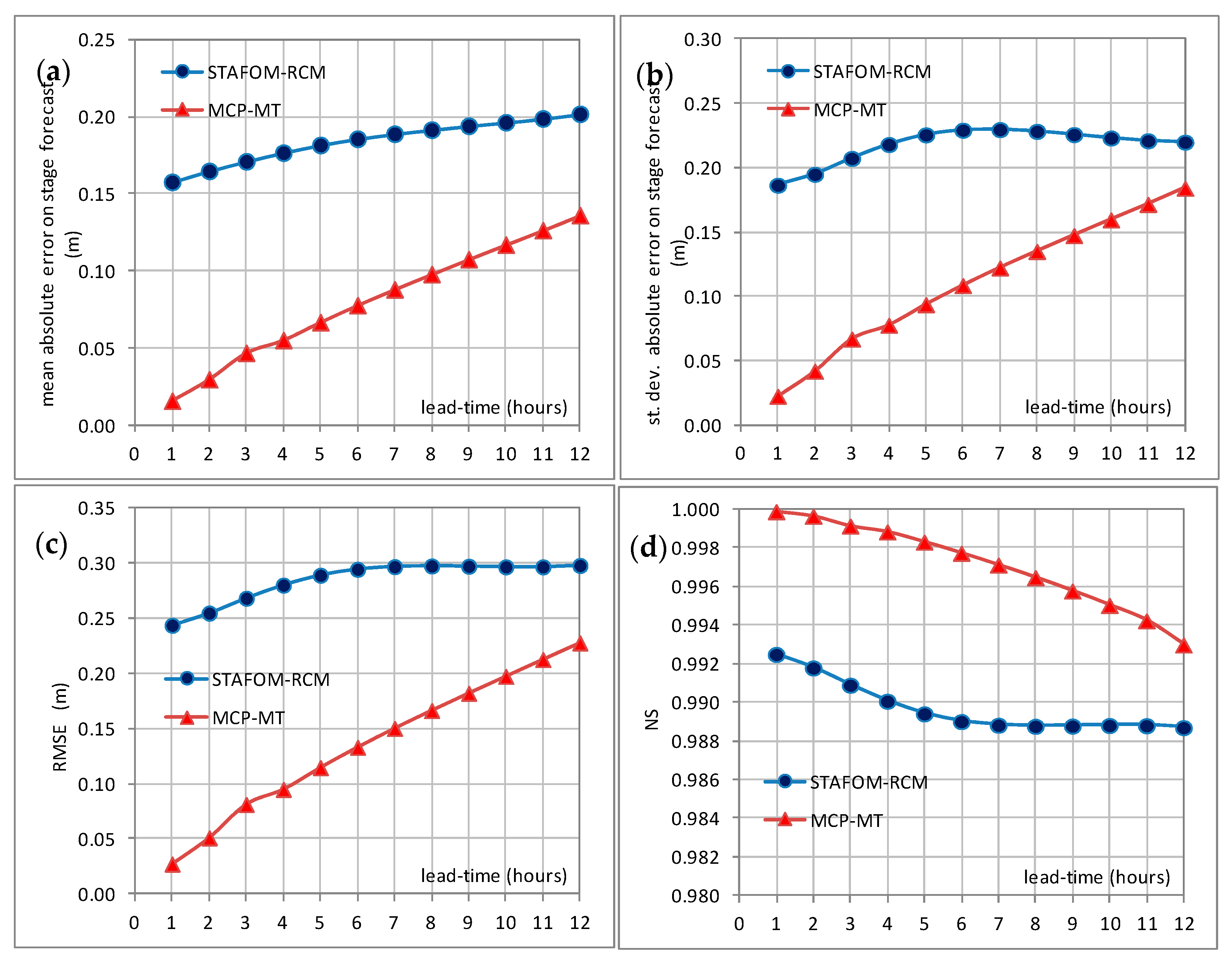
The results of the MCP multi-temporal approach for the two reaches are presented and discussed in the following in terms of the selected performance metrics (i.e., m, σ, RMSE, NS and PC). The analysis is based on the comparison of these evaluation indices computed for the deterministic forecasts and the expected value estimated by MCP-MT. Specifically, the benefits introduced by the PU estimate are discussed: (1) for a forecast horizon of 10 and 12 h for reach 1; and (2) for a lead-time of 20 and 24 h for reach 2.

The effect introduced by MCP-MT can be inferred from Table 2 where a general reduction of the mean absolute error on stage forecast, m, and the root mean square error can be observed for all the lead-times and for both the investigated reaches. Similarly, the standard deviation of the absolute error on stage forecast is lower for MCP-MT expected value than for the deterministic model, with the most significant reduction for the case of reach 2 and lead-time equal to 24 h. Moreover, the NS values, already very high for the model performance, are found improved when the MCP-MT expected value is considered for all the case studies. Finally, a significant increase of PC is observed for both the investigated reaches and all the selected lead-times, with values always higher than 0.55.

The benefit introduced by MCP-MT application can be also seen in Figure 4 where the results of the multi-temporal MCP are compared with those of the deterministic model for all the investigated lead-times for reach 1. The performance of MCP-MT is affected by the accuracy of the deterministic model and, consequently, it decreases with increasing lead-times, as shown in the figure. However, it is worth noting that MCP-MT introduces, compared with the deterministic model, a general reduction of the mean absolute error on stage forecast, m, of its standard deviation and of the RMSE for all the lead-times, while NS values increase. Similar results are observed for the reach 2 case study.

To evaluate the MCP-MT performance, we also compare the percentiles estimated by the processor and the corresponding observed occurrences. This comparison is shown in Figure 6 where the cumulated 0.05 (5%) probability quantiles estimated by the MCP-MT are plotted against the corresponding percentages of observed data that falls below each percentile. Specifically, n_{obs_i} is the number of occurrences below the ith percentile and n is the sample size. The line y = x identifies the perfect behavior (red diagonal), while the deviation from the bisector suggests if the PU estimated percentiles are underestimated or overestimated.

The Figure 6a shows the comparison for the MCP-MT based on the forecasts of STAFOM-RCM for reach 1 and lead-time = 12 h, considering all the available dataset. As it can be seen, the estimated percentiles are found higher than the corresponding observed frequencies up to 50%, while the observed occurrences are greater than the relative PU estimated percentiles in the range 50%–95%. This result indicates that the stage time series estimated by the MCP-MT corresponding to the percentiles between 5% and 50% are underestimated, while the ones referring to percentiles between 50% and 95% seem to be overestimated. As a consequence, the 90% width of the uncertainty band provided by MCP-MT is expected to be overestimated. However, it is worth noting that the deviation of the points from the bisector is quite low and equal on average to about 8%.

Similar considerations apply for the results based on the forecast model application to the longer reach (see Figure 6b) with a mean distance of the points from the red diagonal equal to 7%. Finally, it is important to underline that the 90% uncertainty band provided by MCP-MT is verified, with the percentage of included observed occurrences slightly higher than 90% (

Table 3. Polavaram section (MCP-MT calibrated considering all the available dataset): percentage of observed data that fall inside the 90% uncertainty band (Perc90%), and mean and standard deviation of the uncertainty band width.

River Reach	Lead-Time (h)	Perc90%	Width of the 90% Uncertainty Band
			Mean (m)	Standard Deviation (m)
reach 1	10	93.7	0.73	0.20
	12	93.6	0.84	0.23
reach 2	20	93.1	1.42	0.32
	24	93.2	1.40	0.30

).

Figure 7 and Figure 8 show for some selected case studies the 90% uncertainty band and the expected value assessed by the MCP-MT for reach 1 and reach 2, respectively, along with the forecast of the deterministic model, demonstrating the benefit introduced by the processor application. It can be seen that the PU estimate is able to mitigate the overestimation of STAFOM-RCM forecast for most of the periods when it is observed. Specifically, examples are provided in Figure 7a (first flood wave) and Figure 7b for reach 1 application (lead-time = 10 h) and in Figure 8a,b for reach 2, when a forecast horizon equal to 24 h is considered.

At the same time, the underestimation of the deterministic model forecasts is also addressed by the PU estimate, as can be seen by inspecting the second flood wave shown in Figure 7a and the flood hydrograph depicted in Figure 8b between t = 102 h and t = 138 h.

Figure 7 and Figure 8 show that the observed rising limbs and peak regions are almost included in the 90% uncertainty band for the flood waves represented in the figures.

Furthermore, it is noteworthy that during the flood waves shown in Figure 7 and Figure 8 the observed stage has never reached the alarm threshold, which, properly, is never intersected by the uncertainty band estimated by MCP-MT. As concerns the warning threshold, it is actually exceeded only during the flood of August 2010 (see Figure 8b) as correctly forecasted by both the deterministic model and the MCP-MT uncertainty band.

Finally, the analysis of the width of the 90% uncertainty band is important because it represents a further evaluation measure for investigating the uncertainty reduction with respect to the available information, i.e., the deterministic forecasts. The relevant results computed for the whole used dataset are summarized in Table 3 where the mean and the standard deviation of the width of the 90% uncertainty band provided by MCP-MT are listed for both reaches. When reach 1 is of concern, the mean band width is significantly below 1 m for both 10 and 12 h lead times, with a standard deviation of about 0.2 m. A wider band is assessed for the longer reach and this is expected because the deterministic model error increases; nevertheless, the uncertainty band is on average 1.4 m wide with a low standard deviation of about 0.3 m.

The PU estimate is, definitely, an added value compared to providing only the forecasts of the deterministic model and it is potentially useful for supporting real-time decision-making mainly because it can provide fundamental information on the hydrometric thresholds exceedance probability within the time forecast horizon. Moreover, it could be that the deterministic prediction giving only a single value does not exceed the threshold, while the PU lines overcome the critical level and this surely represents an added value.

5.3.1. Calibration and Validation

In order to better evaluate the performance of MCP-MT for the selected study areas, a division of the whole available data into calibration and validation datasets is also tested. To this end, the dataset is divided by considering the monsoon season of years 2001, 2002, 2003 and 2004 as calibration period and the monsoon season of years 2005, 2007 and 2010 as validation dataset for both the investigated river reaches. Therefore, the calibration time series consists of about 9000 and 10,000 hourly data for reach 1 and reach 2, respectively, while the validation dataset is made up of more than 8000 data for both the investigated Godavari River branches. The main results of this analysis are summarized in Figure 6c–f and in

Table 4. As for Table 2, but considering a separated calibration and validation dataset for MCP-MT.

River Reach	Lead-Time (h)	STAFOM-RCM					MCP-MT Expected Value
		er_h (m)		NS	RMSE (m)	PC	er_h (m)		NS	RMSE (m)	PC
		m	σ				m	σ
Calibration (2001–2004)
reach 1	12	0.184	0.194	0.99	0.267	0.73	0.115	0.137	0.996	0.178	0.88
reach 2	24	0.343	0.400	0.958	0.527	0.4	0.263	0.306	0.975	0.403	0.74
Validation (2005, 2007, 2010)
reach 1	12	0.221	0.243	0.987	0.328	0.58	0.142	0.212	0.992	0.255	0.75
reach 2	24	0.362	0.426	0.958	0.56	0.55	0.292	0.348	0.973	0.455	0.71

and

Table 5. As for Table 3, but considering a separated calibration and validation dataset for MCP-MT.

River Reach	Lead-Time (h)	Perc90%	Width of the 90% Uncertainty Band
			Mean (m)	Standard Deviation (m)
Calibration (2001–2004)
reach 1	12	92.3	0.68	0.22
reach 2	24	92.3	1.33	0.33
Validation (2005, 2007, 2010)
reach 1	12	92.0	0.74	0.20
reach 2	24	92.2	1.4	0.29

.

The benefit introduced by MCP-MT is demonstrated in Table 4 where a general reduction of m and RMSE can be observed for both the investigated reaches and for both the calibration and validation period. Similarly, σ is lower for MCP-MT expected value than for the deterministic model and NS is improved when the MCP-MT expected value is considered. Moreover, an increase of PC is always observed with values higher than 0.7 for MCP-MT.

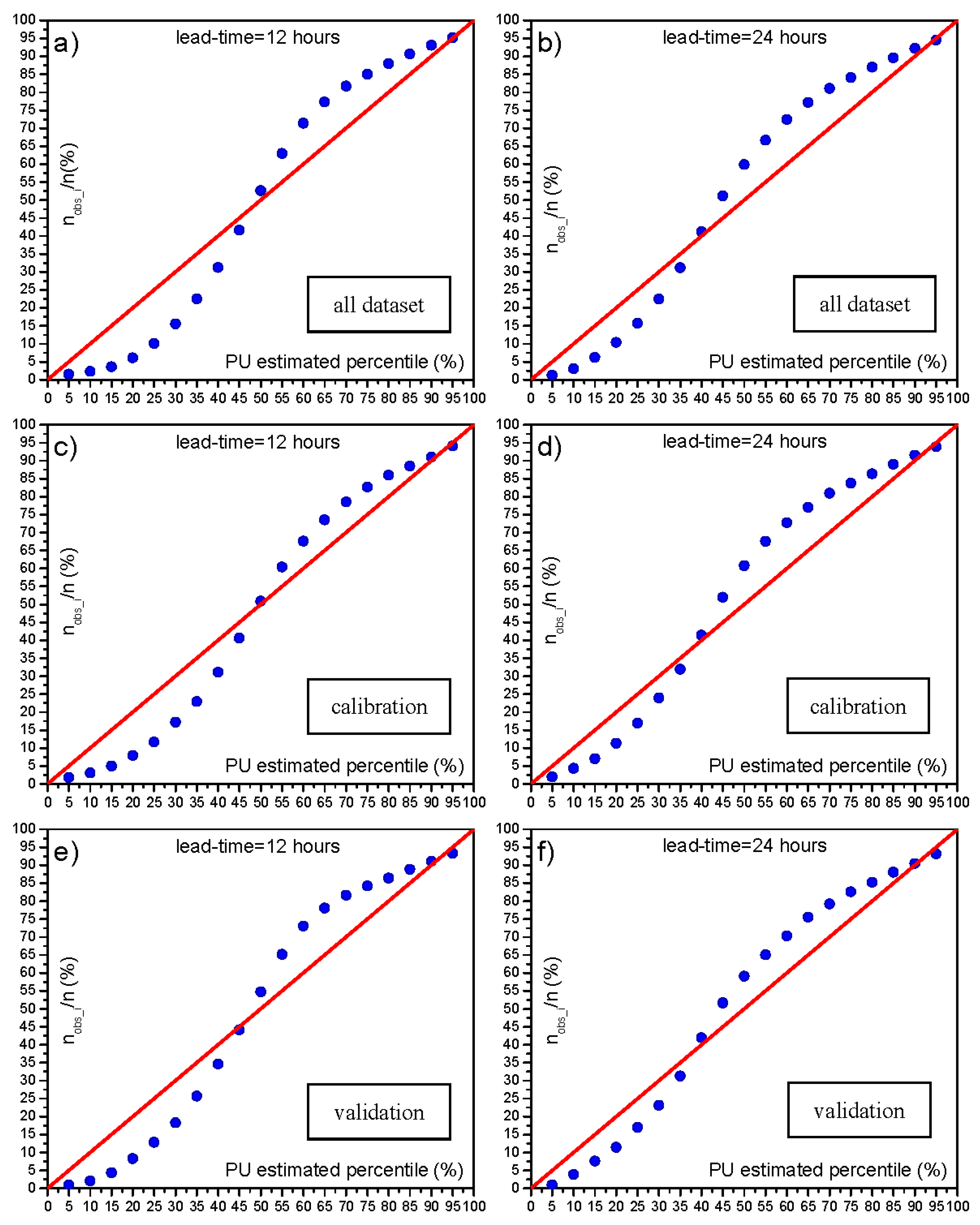
Figure 6c,e shows the comparison between the PU estimated percentiles and the corresponding percentages of observed occurrences falling below each percentile for the MCP-MT based on the forecasts of STAFOM-RCM for reach 1 (lead-time = 12 h), considering the calibration and the validation dataset, respectively. As it can be seen, the PU estimated percentile for the calibration period quite well matches with corresponding observed frequencies, mainly for percentiles higher than 50%. The shape of the curve is similar to the one obtained by calibrating the MCP-MT considering the whole available dataset (Figure 6a) and, hence, analogous considerations hold. It is worth noting that comparable results are achieved also for the validation dataset, shown in Figure 6e. Similar considerations apply to the results based on the forecast model application to the longer reach with a lead-time of 24 h (see Figure 6d,f).

Finally, it is verified that the 90% uncertainty band provided by MCP-MT includes a percentage of observed occurrences slightly higher than 90% (Table 5) and is characterized by very low increase of the mean width from the calibration to the validation dataset, with a slightly decreased standard deviation.

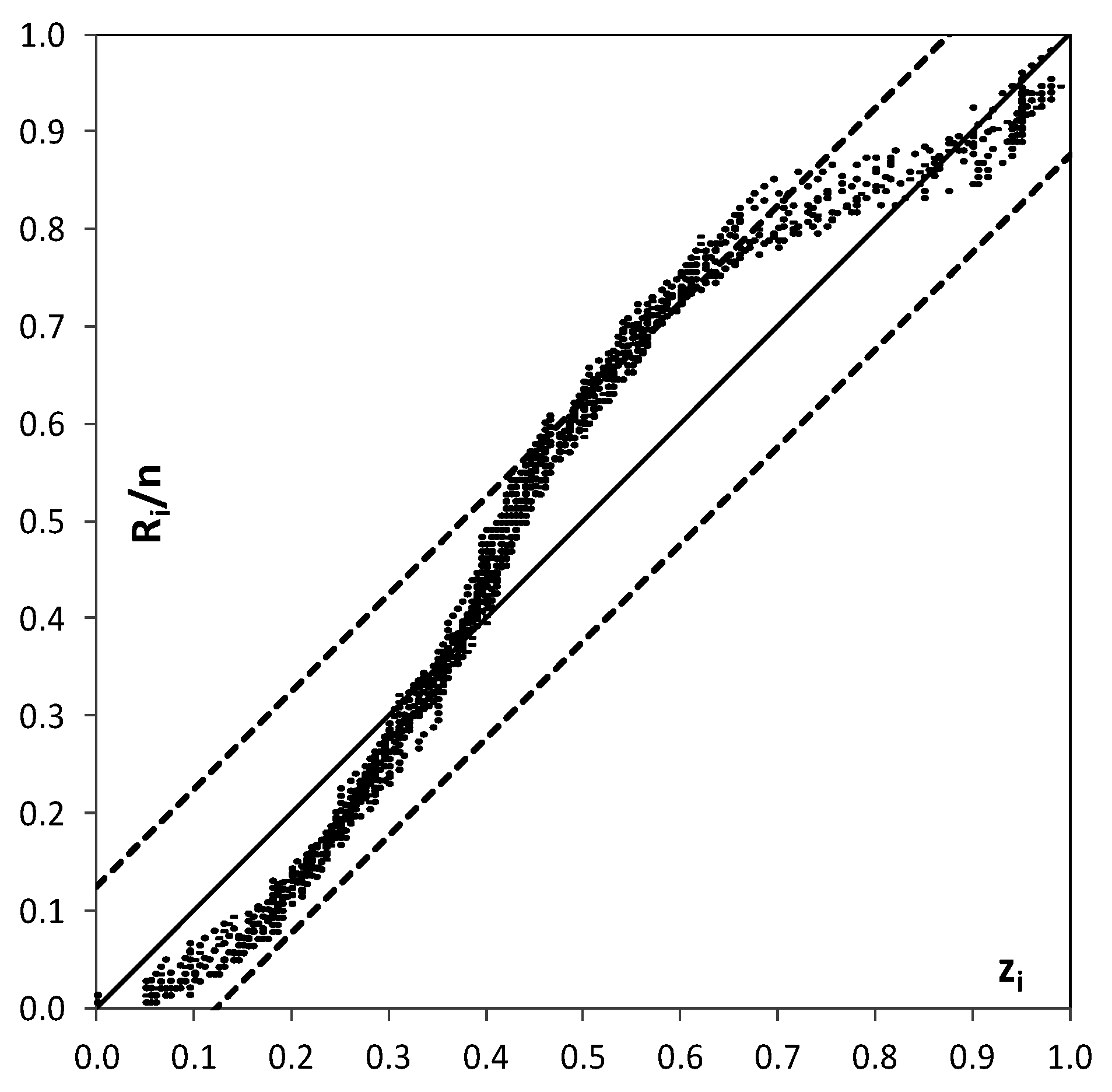
An additional analysis is finally carried out based on the “probability plot representation” (PPR) as described by Laio and Tamea [31]. The PPR is a plot of the values of the forecasted cumulative probability of the observed value x_i, z_i = P(x_i), versus their corresponding empirical distribution function, R_i/n, with R_i = ranks and n = sample size. The PPR indicates if the uniformity test is passed or not and, also, the shape of the resulting curve gives information on the possible causes behind deviations from uniformity, i.e., placement of the points along the 1:1 line [10,31]. Moreover, the Kolmogorov confidence band can be displayed in the PPR indicating if the uniformity test is passed (the curve is inside the band) or not [31]. The PPR is here developed for the case study of MCP-MT results for the longer branch, reach 2, lead-time 24 h and focusing on the 2001 severe monsoon season. Following Laio and Tamea [31], we use 24 sub-series obtaining the results shown in Figure 9. Based on the indications provided by Laio and Tamea [31] to evaluate the results, it is clear that the forecasts provided by the probabilistic method are reliable (most of the forecasts remains inside the Kolmogorov band with 5% significance), even if the shape of the curves indicates that the predictions are large around the central value. The probability plot shows a large steepness of the curves, i.e., more z_i points concentration, in the vicinity of 0.4–0.5 points.

5.3.2. Probability of Hydrometric Thresholds Exceedance: Flooding Probability within a Time Horizon and Contingency Table

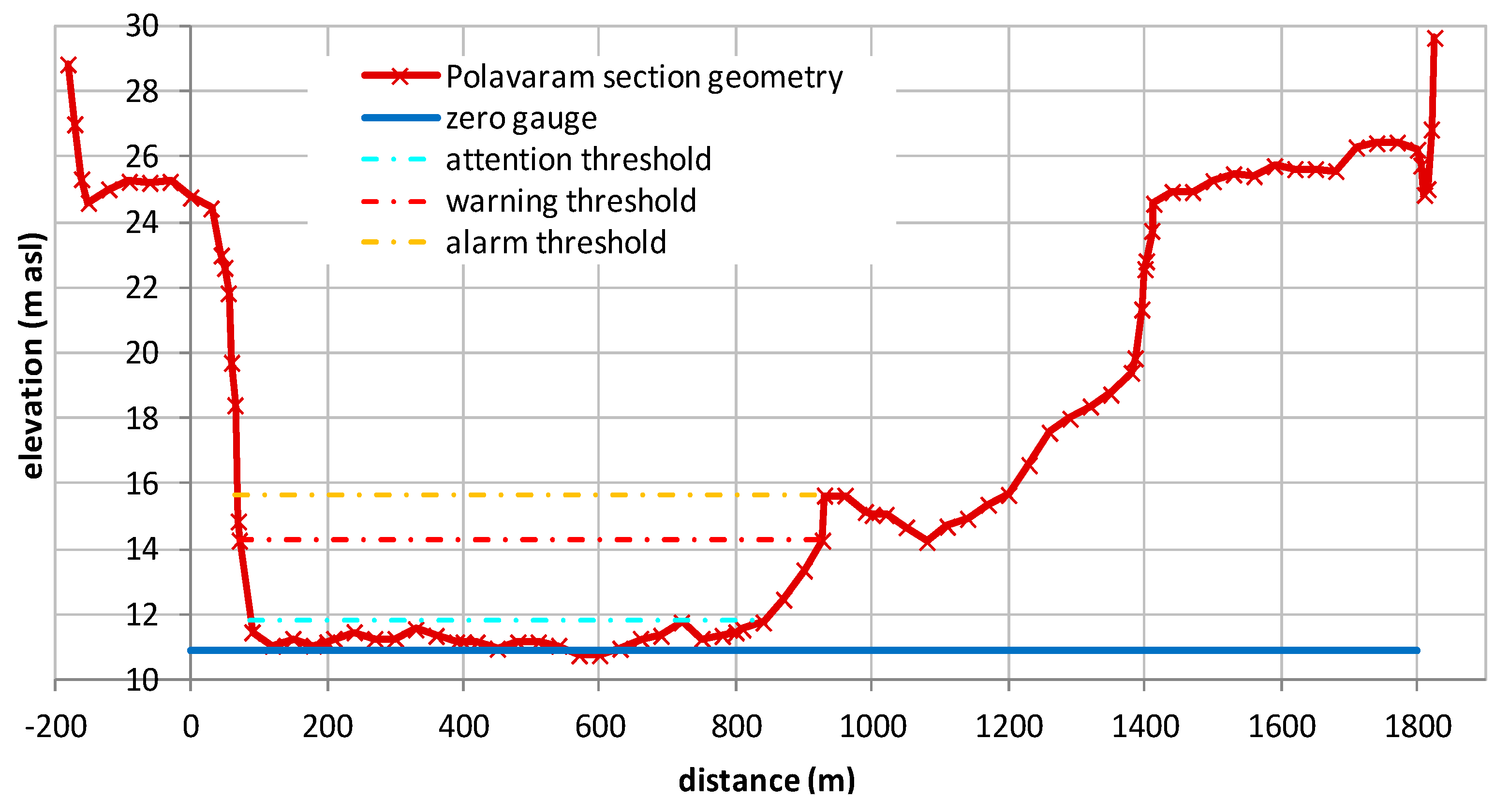
As already underlined, the probability of hydrometric thresholds exceedance (ETP) is fundamental to address the flood risk management in real-time. Therefore, the first results of the MCP-MT in terms of flooding probability are here presented for Polavaram section by assuming as reference thresholds the levels shown in Figure 3 and referred as “attention” (th_att), “warning” (th_war) and “alarm” (th_alar) threshold. It is worth noting that these critical levels are not based on operational values defined by the authority in charge of decision in case of flood, but they are set by the authors. Specifically, the warning and alarm threshold are identified on the basis of the section geometry (see Figure 3), while the lowest one is assumed equal to the 95th percentile of the historical observed river level data with the aim of investigating a critical level exceeded several times during the available dataset.

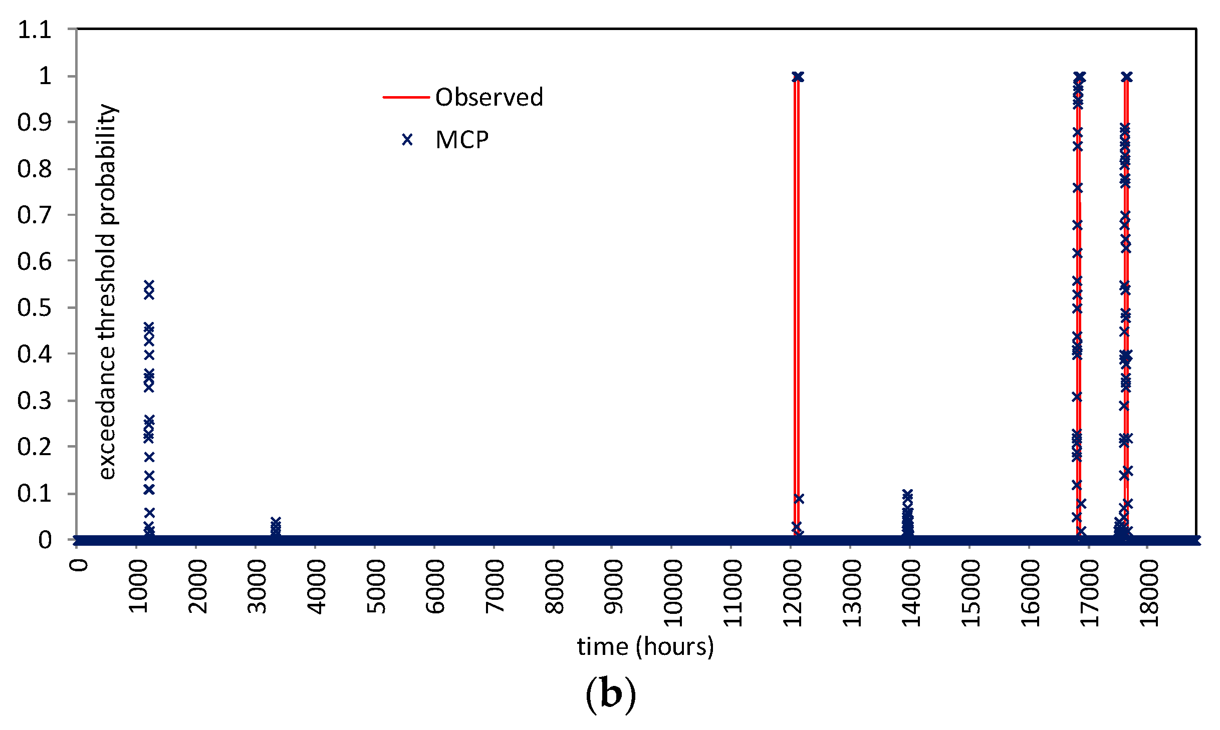
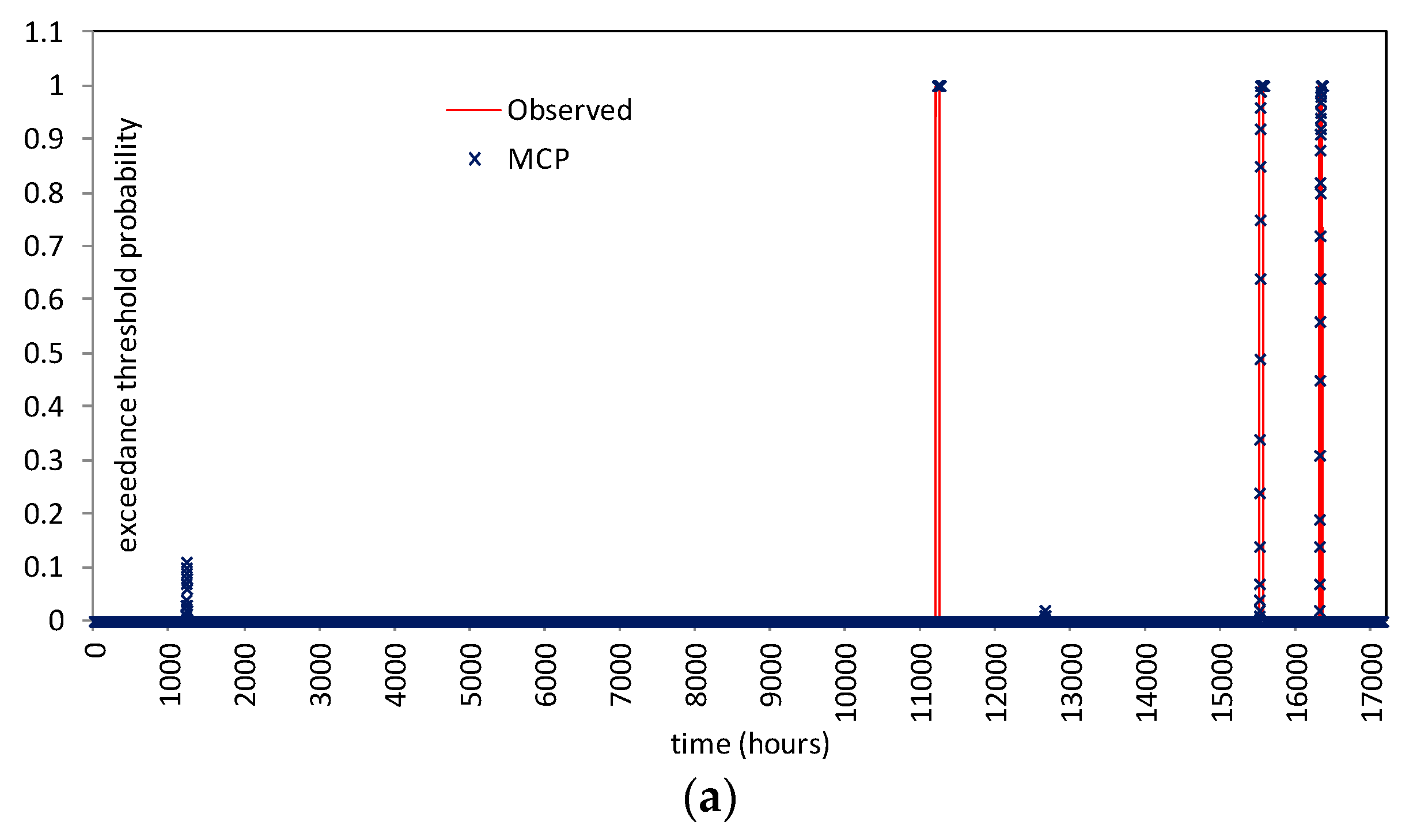
The analysis focuses on the “attention” and “warning” thresholds because the “alarm” threshold is not actually reached during the available dataset. The lead-times of 12 h and 24 h by considering the results of MCP-MT for reach 1 and reach 2, respectively, are selected for the analysis. As for the previous analysis concerning the PU estimate using MCP-MT, we first discuss the results obtained by using the all available dataset for calibration. The study compares the binary observed exceedance, equal to 1 when the observed stage is above the threshold level and equal to 0 when it is below, and the exceeding probability computed by the multi-temporal approach of the MCP-MT within the selected forecast lead-time period. Figure 10 shows the comparison for reach 1 (lead-time = 12 h) and for reach 2 (lead-time = 24 h) for all the available dataset. Specifically, at each time t the displayed value (between 0 and 1) represents the exceedance threshold probability estimated for the next 12/24 h. As it can be seen, when the threshold is really exceeded, the MCP-MT always estimates a probability equal to 1, i.e., provides the certainty of threshold exceeding. When the threshold is not actually exceeded, the processor provides very low probability values, mostly equal to zero. Only in one case, the ETP is found higher than 50% when the threshold is not actually reached (see Figure 10b), however it is worth noting that the maximum observed stage is only 18 centimeters below the threshold level.

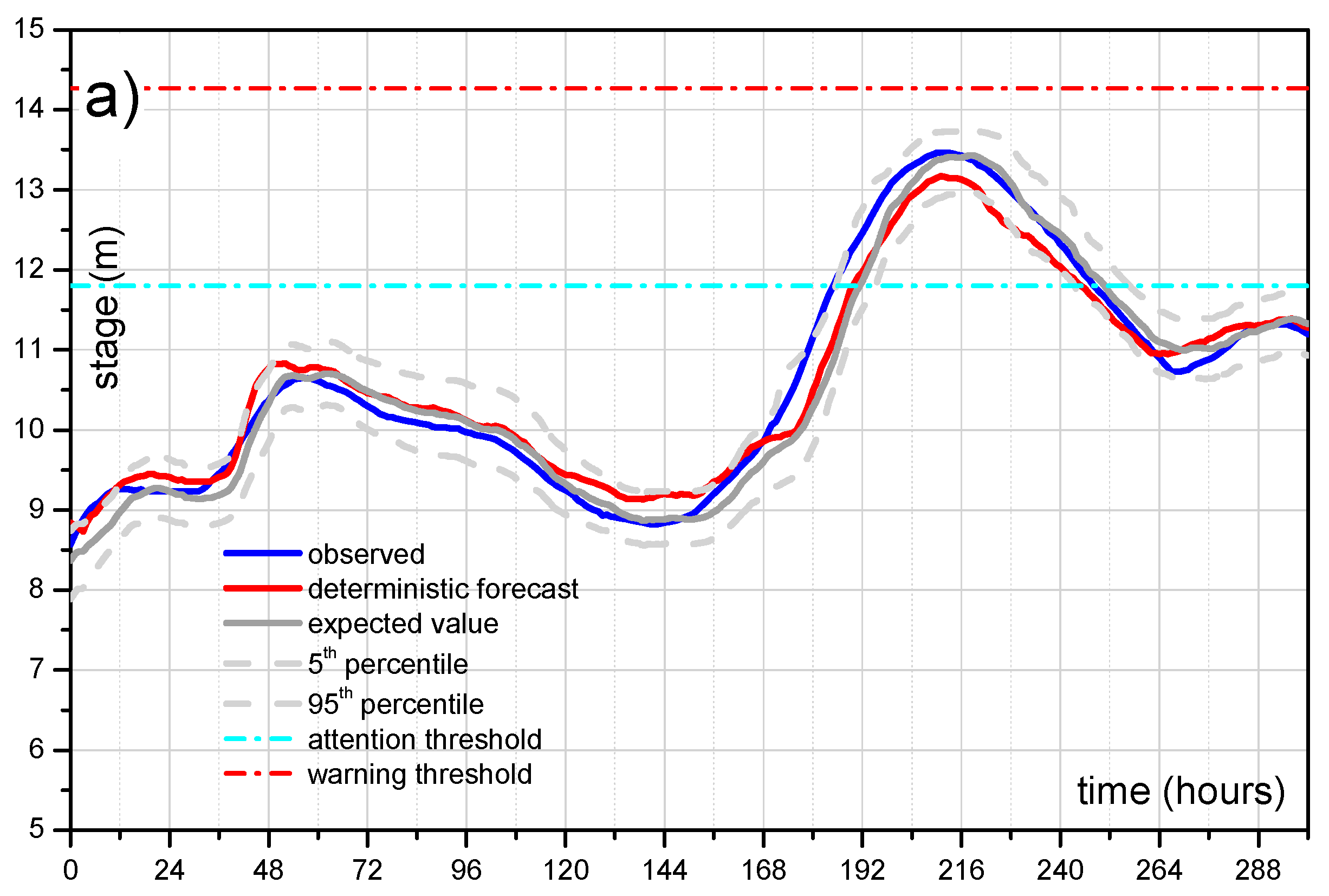
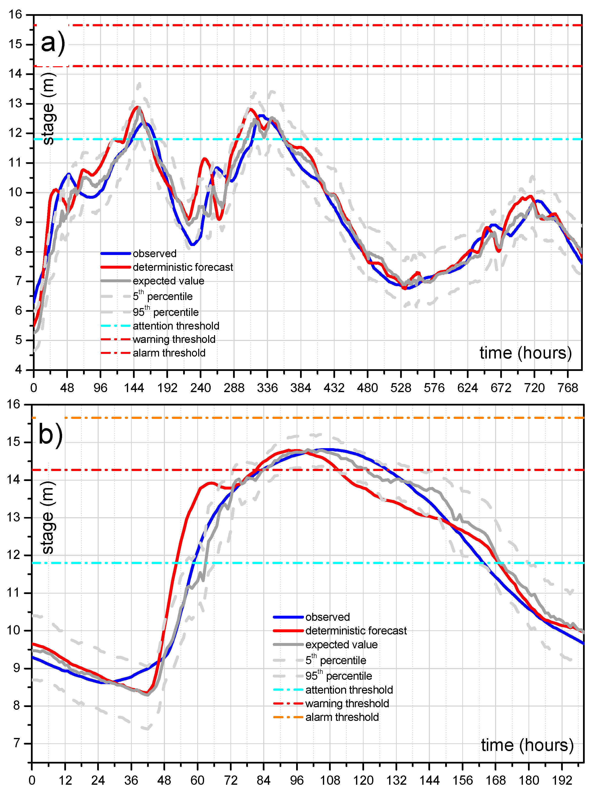
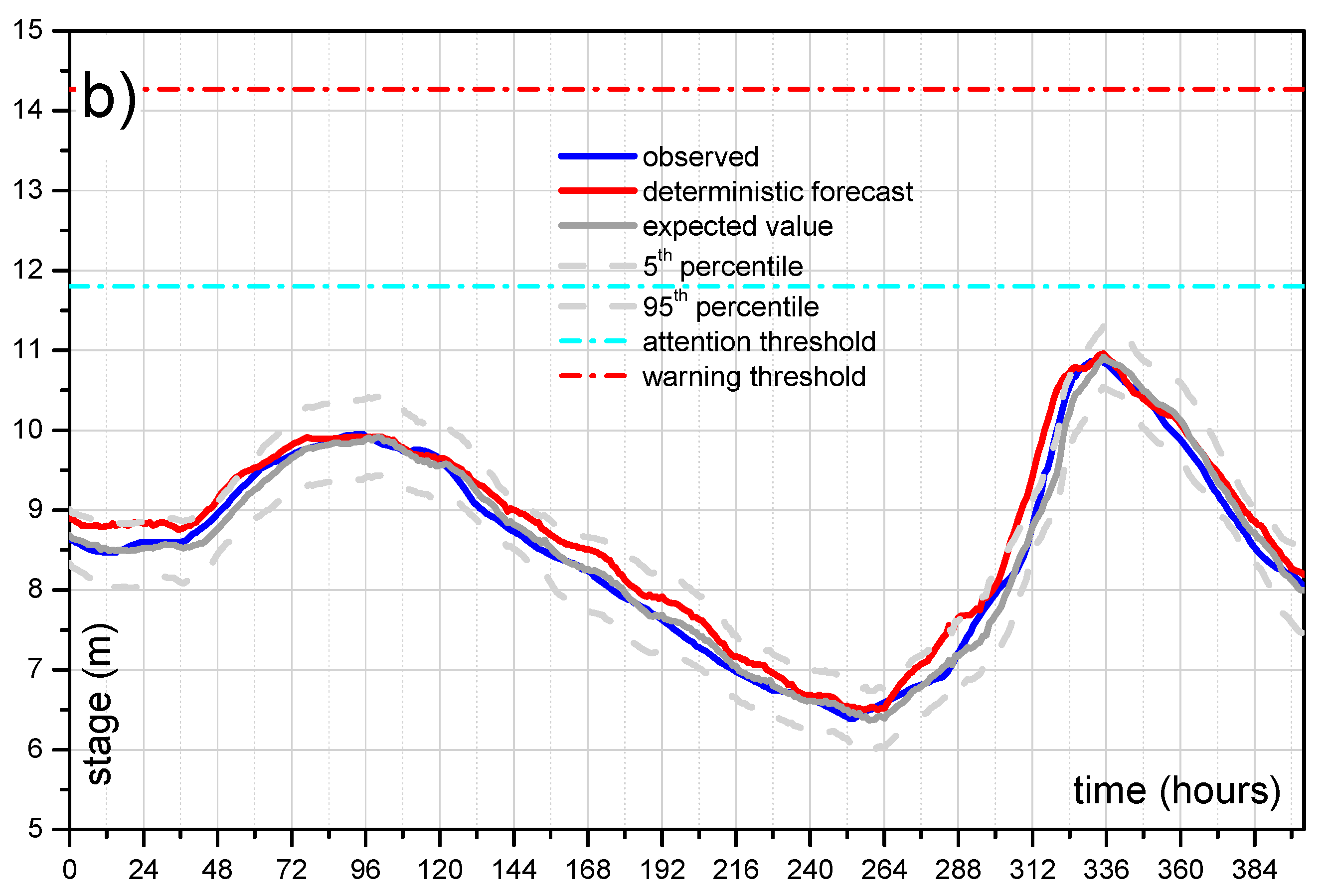
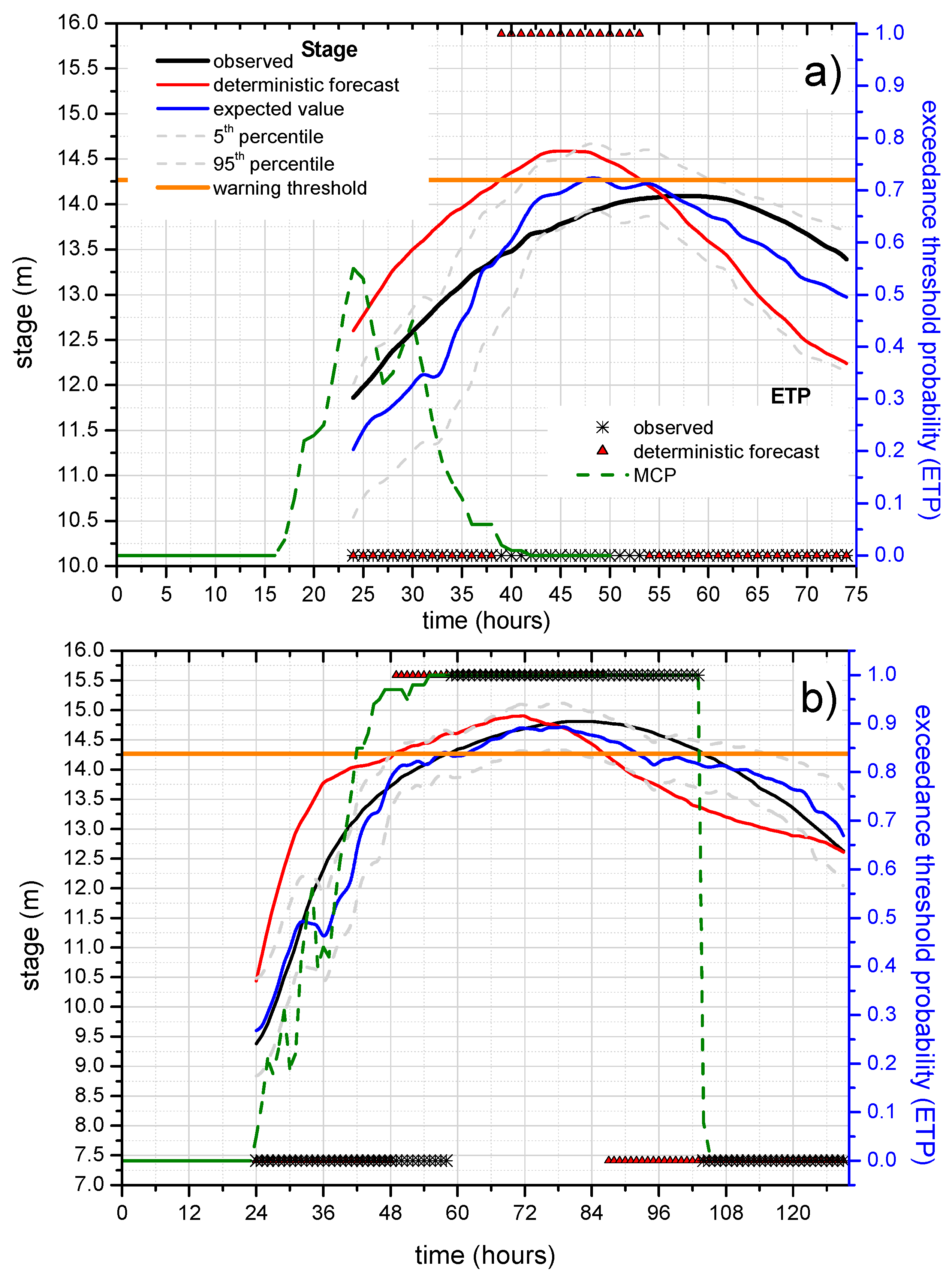
To investigate the benefit of the ETP estimate, a deep analysis on selected flood events is also shown in Figure 11 for the reach 2 case study and the longer lead-time equal to 24 h that represents the best information that could be provided to decision-makers. The analysis consists in comparing the binary observed exceedance (equal to 1 when the observed stage is above the threshold level and equal to 0 when it is below) and the exceeding probability computed by the MCP-MT within the selected forecast lead-time period (24 h) that is varying over time. For sake of completeness, the binary response of the deterministic model, that can be equal to 1 or 0, is also considered in the analysis. Figure 11a,b, which concerns two high flood events occurred at Polavaram section, shows the benefit obtainable using the PU estimate. Specifically, these figures effectively show the advantage of using probabilistic approaches able to provide probabilities in the range of 0–1 and not only the binary values 0/1, corresponding to the condition of threshold exceedance/non-exceedance.

In the figures, the red line represents the stage predicted by STAFOM-RCM model 24 h in advance compared with the observed stage (black line), the expected value (blue line) and the 90% uncertainty band (dashed grey lines) provided by MCP-MT. The dashed green line in Figure 11a,b represents the probability to exceed the level of 14.27 m (warning threshold) within the total time horizon (i.e., 24 h) computed by the MCP-MT. Specifically, the exceedance probability provided by the MCP-MT for each time step t refers to the next 24 h period, i.e., the time interval t–(t + 24 h). As it can be seen, for the flood on 21–22 August 2001 (Figure 11a) the deterministic model predicts the threshold exceedance at time t = 39 h, while the warning threshold was not actually exceeded by the observed stage. In this case, the exceedance probability provided by MCP-MT reaches the maximum value equal to 0.55 at t = 24 h, therefore the ETP is always significanlty lower than 0.75 that identified the limit value for the “red probability class” that indicates a high probability of threshold overtopping. In details, the probability values computed by the MCP-MT can be grouped in three probability classes: the green class refers to the probability lower than 0.25, the red one includes the probability values greater than 0.75 and the yellow class indicates values within these two percentages. The probability classes are assumed to be easily understandable by authorities in charge of decision, providing useful information for supporting the real-time flood risk management.

It is worth noting that the highest values of ETP, between t = 22 h and t = 31 h (see Figure 11a), correspond to the beginning of the peak region of the observed stage hydrograph and that the maximum observed stage is only 18 centimeters lower than the warning threshold.

By inspecting the results shown for the flood which occurred on 6–10 August 2010 (Figure 11b), it can be noted that the warning threshold is actually exceeded at t = 58 h, while the deteministic model predicts the threshold overtopping 9 h in advance, at t = 49 h. The benefit introduced by the predictive uncertatinty estimate can be easily inferred by analyzing the results for the flood of August 2010 (see Figure 11b). In this case, the ETP increases very quickly starting from t = 24 h and reaches nearly the maximum value equal to 1 at t = 47 h. Moreover, the expected value, depicted as the blue line in the figure, passes the threshold at time t = 57 h, only one hour before the actual overtopping.

It is also worth noting that the alarm hydrometric threshold, equal to 15.65 m, is never really exceeded for the whole available dataset and that the ETP provided by MCP-MT for both the investigated reaches is always null for this highest threshold.

Finally, it is worth noting that the probabilistic information from the multi-temporal approach of the MCP-MT refers to the entire forecast horizon, i.e., to a 24 h time interval, while the deterministic models cannot provide exceedance probability.

The contingency table metric [32] is also used to investigate how correctly the exceedance or non-exceedance of the fixed hydrometric thresholds is forecasted. A perfect forecast would produce only “hits” (event forecast to occur, and did occur) and “correct negatives” (event forecast not to occur, and did not occur) and no “misses” (event forecast not to occur, but did occur) or “false alarms” (event forecast to occur, but did not occur).

Table 6. Contingency tables showing the capability of STAFOM-RCM and of the expected value and the 95th percentile provided by MCP-MT in hydrometric thresholds exceedance/non-exceedance prediction.

River Reach		Warning Threshold (14.27 m)			Attention Threshold (11.80 m)
		Hits	False Alarms	Misses	Hits	False Alarms	Misses
		All Dataset (2001–2010)
reach 1 (12 h)	STAFOM-RCM	3	2	0	14	1	0
	Exp. value	3	0	0	14	1	0
	95th perc.	3	2	0	14	1	0
reach 2 (24 h)	STAFOM-RCM	2	1	1	15	2	0
	Exp. value	2	1	1	14	1	1
	95th perc.	3	2	0	15	2	0
		Calibration (2001–2004)
reach 1 (12 h)	STAFOM-RCM	0	1	0	5	0	0
	Exp. value	0	0	0	5	0	0
	95th perc.	0	1	0	5	0	0
reach 2 (24 h)	STAFOM-RCM	0	1	0	6	1	0
	Exp. value	0	0	0	6	0	0
	95th perc.	0	0	0	6	1	0
		Validation (2005, 2007, 2010)
reach 1 (12 h)	STAFOM-RCM	3	1	0	9	1	0
	Exp. value	3	0	0	9	1	0
	95th perc.	3	1	0	9	1	0
reach 2 (24 h)	STAFOM-RCM	2	0	1	9	1	0
	Exp. value	2	0	1	8	1	1
	95th perc.	2	0	1	9	1	0

shows the outcomes of the analysis for the warning and the attention threshold for reach 1 and reach 2 by assuming a lead-time of 12 and 24 h, respectively. The performance of the deterministic model is here compared with the one of the expected value and the 95th percentile provided by MCP-MT. The table provides the hits, the misses and the false alarms, while the correct negatives refer to all the other situations not quantified because during the monsoon season continuous flood events are recorded. As it can be seen, STAFOM-RCM correctly forecasts the three actual warning threshold exceedances with a forecast horizon of 12 h, but also provied two false alarms; when the 24 h lead-time is considered one miss is observed. Referring to th_att, we see 14 hits and one false alarm for 12 h lead-time and 15 hits and two false alarms for 24 h lead-time. By inspecting the results for MCP-MT calibrated by using the whole available dataset, a better performance can be seen both in terms of mean and 95th percentile. For example, the two false alarms for th_war and 12 h lead-time are no more observed for the expected value. Moreover, the two false alarms for reach 2 (24 h) of the 95th percentile are characterized by a maximum value of the exceedance probability provided by MCP-MT lower than 40% and 10%. It is also worth noting that the maximum water level observed during the only miss for th_att provided by the expected value of MCP-MT is found only two centimeters above the critical level.

For a comprehensive evaluation, the anlaysis of how correctly the exceedance or non-exceedance of the fixed hydrometric thresholds is forecasted is also carried out for study based on separated calibration and validation periods. As it can be inferred from Table 6, the warning threshold is never exceeded during the selected calibration period, while it is for three times during the validation period. Nevertheless, MCP-MT expected value and 95th percentile correctly forecast the three threshold exceedances for lead time = 12 h, while for 24 h a miss is observed for which the 95th percentile line is only 10 centimeters below th_war. As concerns th_att, the theshold is reached five and nine times during the calibration and the validation period, respectively, when the dataset of reach 1 is considered. If reach 2 is investigated, it is seen that th_att is exceeded six times during the calibration period and nine times in the validation time series. The results of reach 1 (lead-time = 12 h) show for the calibration period five hits with 0 false alarms and misses (for both the deteministic model and the MCP-MT outcomes), and for the validation period, nine. Threrefore, the th_att overcoming is always correctly predicted when it actually occurs, however one false alarm is also observed in the validation period for MCP-MT as well as for the deterministic model. When the 24 h lead-time case study is analyzed, it is seen that in the calibration period six hits are obtained and only one false alarm for the 95th percentile that, however, is characterized by a maximum probability threshold exceedance equal to 22%. Finally, for the validation dataset, eight and nine hits are found for the expected value and the 95th percentile, respectively, with one miss for the mean of MCP-MT and one false alarm for both that is characterized by a maximum exceedance probability of about 50%.

Based on these results, it is evident that the information provided by the PU estimate with MCP-MT represent an added value to correctly support the activities of real-time FFWSs.

As it can be expected, a better perfomance of the processor is found when it is calibrated on the all available dataset, but even when separated calibration and validation periods are considered, the outcomes suggest that MCP-MT can be conveniently used for addressing flood risk management.

6. Conclusions

This paper presents the application of the multi-temporal approach of the Model Conditional Processor, MCP-MT, for a study area selected in the Godavari River basin, India. The MCP-MT uses several lead-time forecasts provided by deterministic forecasting models and estimates the Predictive Uncertainty (PU) through a generalized form of the Bayes theorem. The processor is here applied for two case studies selected in the Godavari River basin, India, with the aim of verifying the benefits that could result from the PU estimate within the FFWS of this area, located in a developing country that is fully based on real-time observations and deterministic forecasts without uncertainty estimation. The analysis is carried out by exploiting the first application of the STAFOM-RCM forecasting model to two selected Godavari River reaches: Perur-Polavaram reach and Bhadrachalam-Polavaram branch. The former, 206 km long, is characterized by a mean wave travel time, assumed as the characteristic lead-time, between 20 and 24 h, while the latter is shorter (73 km) with a characteristic lead-time between 10 and 12 h.

Specifically, the study is performed on a dataset of 19,294 and 17,339 hourly stage data for Perur-Polavaram and Bhadrachalam-Polavaram, respectively, selected during the monsoon season (June–October) for the period 2001–2010.

The analysis was first carried out considering the entire dataset for MCP-MT calibration, but the performance was also investigated considering separated calibration and validation periods.

The results show that the deterministic forecasts provided by the flood routing model named STAFOM-RCM are accurate for the selected lead-times with very high values of the NS coefficient, always higher than 0.95, and low errors on stage forecast. Even if the results may indicate that the model could support the operative flood forecasting activity in the Godavari River basin, the PU estimation is the fundamental added value for the present early warning system. The PU assessed through MCP-MT is found to provide useful information on the hydrometric thresholds exceedance probability within the time horizon, demonstrating the potential usefulness for supporting real-time decision-making.

The first application of the MCP-MT indicates that the expected value of the predictand conditional on the deterministic model forecasts already improves over the original model predictions. Specifically, MCP-MT introduces a general reduction of the mean absolute error on stage forecast and of the root mean square error for all the lead-times and for both the investigated reaches. Similarly, the standard deviation of the absolute error on stage forecast decreases for MCP-MT expected value compared with the one of the deterministic model, while NS increases for all the case studies. Moreover, the 90% uncertainty band provided by MCP-MT is verified, with the percentage of included observed occurrences slightly higher than 90%.

Overall, the first promising results indicate that the MCP-MT could be an appropriate solution for the operational community of the Godavari River basin who would adopt probabilistic forecasting framework without spending significant resources.

References

1. Pappenberger, F.; Cloke, H.L.; Parker, D.J.; Wetterhall, F.; Richardson, D.S.; Thielen, J. The monetary benefit of early flood warnings in Europe. Environ. Sci. Policy 2015, 51, 278–291. [Google Scholar] [CrossRef]
2. Krzysztofowicz, R. Bayesian system for probabilistic river stage forecasting. J. Hydrol. 2002, 268, 16–40. [Google Scholar] [CrossRef]
3. Todini, E. Role and treatment of uncertainty in real-time flood forecasting. Hydrol. Process. 2004, 18, 2743–2746. [Google Scholar] [CrossRef]
4. Clark, M.P.; Slater, A.G. Probabilistic quantitative precipitation estimation in complex terrain. J. Hydrometeorol. 2006, 7, 3–22. [Google Scholar] [CrossRef]
5. Vrugt, J.A.; Robinson, B.A. Treatment of uncertainty using ensemble methods: Comparison of sequential data assimilation and Bayesian model averaging. Water Resour. Res. 2007, 43, W01411. [Google Scholar] [CrossRef]
6. Ebtehaj, M.; Moradkhani, H.; Gupta, H.V. Improving robustness of hydrologic parameter estimation by the use of moving block bootstrap resampling. Water Resour. Res. 2010, 46, W07515. [Google Scholar] [CrossRef]
7. He, X.; Refsgaard, J.C.; Sonnenborg, T.O.; Vejen, F.; Jensen, K.H. Statistical analysis of the impact of radar rainfall uncertainties on water resources modeling. Water Resour. Res. 2011, 47, W09526. [Google Scholar] [CrossRef]
8. Legleiter, C.J.; Kyriakidis, P.C.; McDonald, R.R.; Nelson, J.M. Effects of uncertain topographic input data on twodimensional flow modeling in a gravel-bed river. Water Resour. Res. 2011, 47, W03518. [Google Scholar] [CrossRef]
9. Sikorska, A.E.; Scheidegger, A.; Banasik, K.; Rieckermann, J. Bayesian uncertainty assessment of flood predictions in ungauged urban basins for conceptual rainfall-runoff models. Hydrol. Earth Syst. Sci. 2012, 16, 1221–1236. [Google Scholar] [CrossRef]
10. Montanari, A.; Koutsoyiannis, D. A blueprint for process-based modeling of uncertain hydrological systems. Water Resour. Res. 2012, 48, W09555. [Google Scholar] [CrossRef]
11. Montanari, A.; Grossi, G. Estimating the uncertainty of hydrological forecasts: A statistical approach. Water Resour. Res. 2008, 44, W00B08. [Google Scholar] [CrossRef]
12. Smith, P.J.; Beven, K.J.; Weerts, A.H.; Leedal, D. Adaptive correction of deterministic models to produce accurate probabilistic forecasts. Hydrol. Earth Syst. Sci. 2012, 16, 2783–2799. [Google Scholar] [CrossRef] [Green Version]
13. Hoss, F.; Fischbeck, P.S. Performance and robustness of probabilistic river forecasts computed with quantile regression based on multiple independent variables. Hydrol. Earth Syst. Sci. 2015, 19, 3969–3990. [Google Scholar] [CrossRef]
14. Krzysztofowicz, R. Bayesian theory of probabilistic forecasting via deterministic hydrologic model. Water Resour. Res. 1999, 35, 2739–2750. [Google Scholar] [CrossRef]
15. Krzysztofowicz, R.; Kelly, K.S. Hydrologic uncertainty processor for probabilistic river stage forecasting. Water Resour. Res. 2000, 36, 3265–3277. [Google Scholar] [CrossRef]
16. Coccia, G.; Todini, E. Recent development in predictive uncertainty assessment based on the model conditional processor approach. Hydrol. Earth Syst. Sci. 2011, 15, 3253–3274. [Google Scholar] [CrossRef]
17. Raftery, A.E. Bayesian model selection in structural equation models. In Testing Structural Equation Models; Bollen, K.A., Long, J.S., Eds.; Sage: Beverly Hills, CA, USA, 1993; pp. 163–180. [Google Scholar]
18. Raftery, A.E.; Balabdaoui, F.; Gneiting, T.; Polakowski, M. Using Bayesian model averaging to calibrate forecast ensembles. Mon. Weather Rev. 2005, 133, 1155–1174. [Google Scholar] [CrossRef]
19. Todini, E. A model conditional processor to assess predictive uncertainty in flood forecasting. Int. J. River Basin Manag. 2008, 6, 123–137. [Google Scholar] [CrossRef]
20. Plate, E.J.; Shahzad, K.M. Uncertainty Analysis of Multi-Model Flood Forecasts. Water 2015, 7, 6788–6809. [Google Scholar] [CrossRef]
21. Coccia, G. Analysis and Developments of Uncertainty Processors for Real Time Flood Forecasting. Ph.D. Thesis, Alma Mater Studiorum University of Bologna, Bologna, Italy, 2011. [Google Scholar]
22. Barbetta, S.; Moramarco, T.; Franchini, M.; Melone, F.; Brocca, L.; Singh, V.P. Case Study: Improving real-time stage forecasting Muskingum model by incorporating the Rating Curve Model. J. Hydrol. Eng. 2011, 16, 540–557. [Google Scholar] [CrossRef]
23. Van der Waerden, B.L. Order tests for two-sample problem and their power I. Indag. Math. 1952, 14, 453–458. [Google Scholar] [CrossRef]
24. Van der Waerden, B.L. Order tests for two-sample problem and their power II. Indag. Math. 1953, 15, 303–310. [Google Scholar] [CrossRef]
25. Van der Waerden, B.L. Order tests for two-sample problem and their power III. Indag. Math. 1953, 15, 311–316. [Google Scholar] [CrossRef]
26. Barbetta, S.; Moramarco, T.; Brocca, L.; Franchini, M.; Melone, F. Confidence interval of real-time forecast stages provided by the STAFOM-RCM model: The case study of the Tiber River (Italy). Hydrol. Process. 2014, 28, 729–743. [Google Scholar] [CrossRef]
27. Moramarco, T.; Barbetta, S.; Melone, F.; Singh, V.P. Relating local stage and remote discharge with significant lateral inflow. J. Hydrol. Eng. 2005, 10, 58–69. [Google Scholar] [CrossRef]
28. Barbetta, S.; Franchini, M.; Melone, F.; Moramarco, T. Enhancement and comprehensive evaluation of the Rating Curve Model for different river sites. J. Hydrol. 2012, 464–465, 376–387. [Google Scholar] [CrossRef]
29. Nash, J.E.; Sutcliffe, J.V. River flow forecasting through conceptual models, Part I: A discussion of principles. J. Hydrol. 1970, 10, 282–290. [Google Scholar] [CrossRef]
30. Kitanidis, P.K.; Bras, R. Real time forecasting with a conceptual hydrologic model. 2. Applications and results. Water Resour. Res. 1980, 16, 1034–1044. [Google Scholar] [CrossRef]
31. Laio, F.; Tamea, S. Verification tools for probabilistic forecasts of continuous hydrological variables. Hydrol. Earth Syst. Sci. 2007, 11, 1267–1277. [Google Scholar] [CrossRef]
32. Wilks, D.S. Statistical Methods in Atmospheric Sciences, 2nd ed.; Academic Press: San Diego, CA, USA, 2006. [Google Scholar]
Figure 1. Schematic diagram of the four main steps of the MCP for Predictive Uncertainty estimate.
Water 08 00463 g001
Figure 2. Morphology of the Godavari River with the location of the hydrometric monitoring network.
Water 08 00463 g002
Figure 3. Godavari River: geometry of the Polavaram section where the stage forecast and the PU estimate are provided. The zero gauge level is shown along with the assumed hydrometric thresholds.
Water 08 00463 g003
Figure 4. Godavari River, reach 1 (Bhadrachalam-Polavaram): performance measures for the deterministic forecast and the MCP-MT application for lead-times from 1 to 12 h: (a) mean of the absolute error on stage forecast; (b) standard deviation of the absolute error on stage forecast; (c) root mean square error, RMSE; and (d) Nash–Sutcliffe coefficient, NS. The measures are computed for the entire database.
Water 08 00463 g004
Figure 5. Division of the joint distribution in the transferred normal space (i.e., space fulfilling assumptions of normality) into two bivariate truncated normal distributions for: (a) Bhadrachalam-Polavaram reach (lead-time = 12 h); and (b) Perur-Polavaram reach (lead-time = 24 h). The red line represents the mean value, while the light blue lines represent the 5% and the 95% quantiles. The black dashed line represents the threshold used in order to identify the two TNDs.
Water 08 00463 g005
Figure 6. Comparison between the MCP-MT estimated percentiles and the corresponding observed occurrences (nobs_i = number of occurrences below the ith percentile, n = sample size) for: (a,b) all calibration dataset ((a) reach 1; and (b) reach 2); (c,d) calibration period 2001–2004 ((c) reach 1; and (d) reach 2); and (e,f) validation period 2005, 2007 and 2010 ((e) reach 1; and (f) reach 2). The red line represents the perfect behavior, and the blue shows the MCP-MT response.
Water 08 00463 g006
Figure 7. Polavaram section (lead-time = 12 h): comparison between observed and forecast stages provided STAFOM-RCM applied to the shorter reach for the flood event occurred on the period: (a) 19–31 July 2003; and (b) 10–27 August 2004. The 90% uncertainty band along with the expected value assessed through the multi-temporal approach of MCP-MT are also shown.
Water 08 00463 g007aWater 08 00463 g007b
Figure 8. As for Figure 7, but for STAFOM-RCM applied to the longer reach (lead-time = 24 h) and for the events occurred on the period: (a) 24 July–26 August 2005; and (b) 4–12 August 2010.
Water 08 00463 g008
Figure 9. Godavari River, monsoon season 2001 (reach 2, lead-time = 24 h): probability plot representation of the probabilistic forecast. The Kolmogorov 5% significance band is shown as dashed lines.
Water 08 00463 g009
Figure 10. Polavaram section (warning threshold = 14.27 m): comparison between the observed exceedance threshold probability and the one computed by the MCP-MT within: (a) the next 12 h (reach 1); and (b) the next 24 h (reach 2) for all the available dataset.
Water 08 00463 g010aWater 08 00463 g010b
Figure 11. Polavaram section (lead-time 24 h): overtopping warning threshold exceedance probability within the following 24 h estimated by MCP-MT (the threshold exceedance probability at time t refers to the interval tt + 24 h) for the flood occurred on: (a) 21–22 August 2001; and (b) 6–10 August 2010. The comparison between deterministic and probabilistic stage forecasts is also shown along with the observed occurrences.
Water 08 00463 g011