
A Spaceborne Multisensory, Multitemporal Approach to Monitor Water Level and Storage Variations of Lakes


Abstract
:1. Introduction
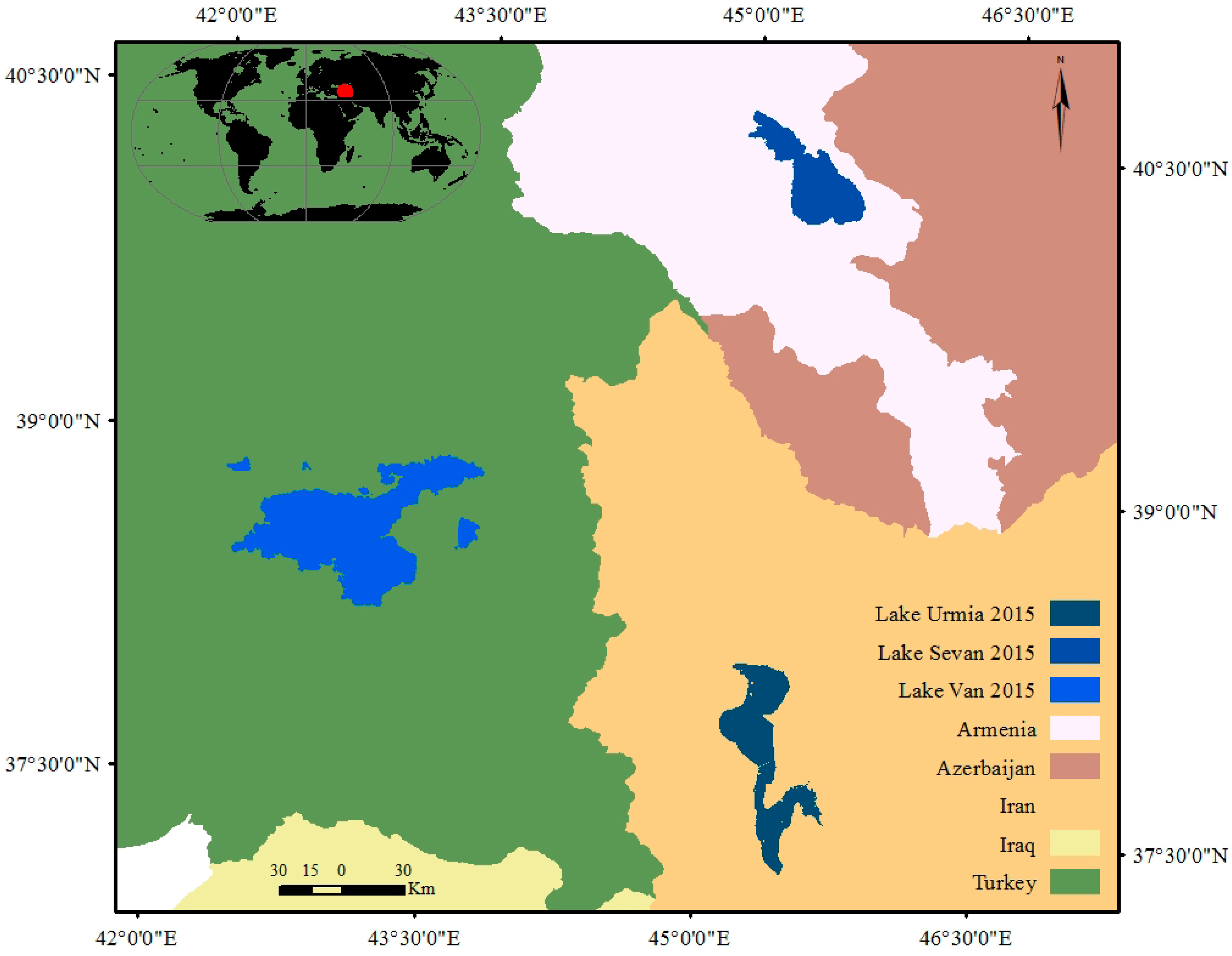
2. Study Areas
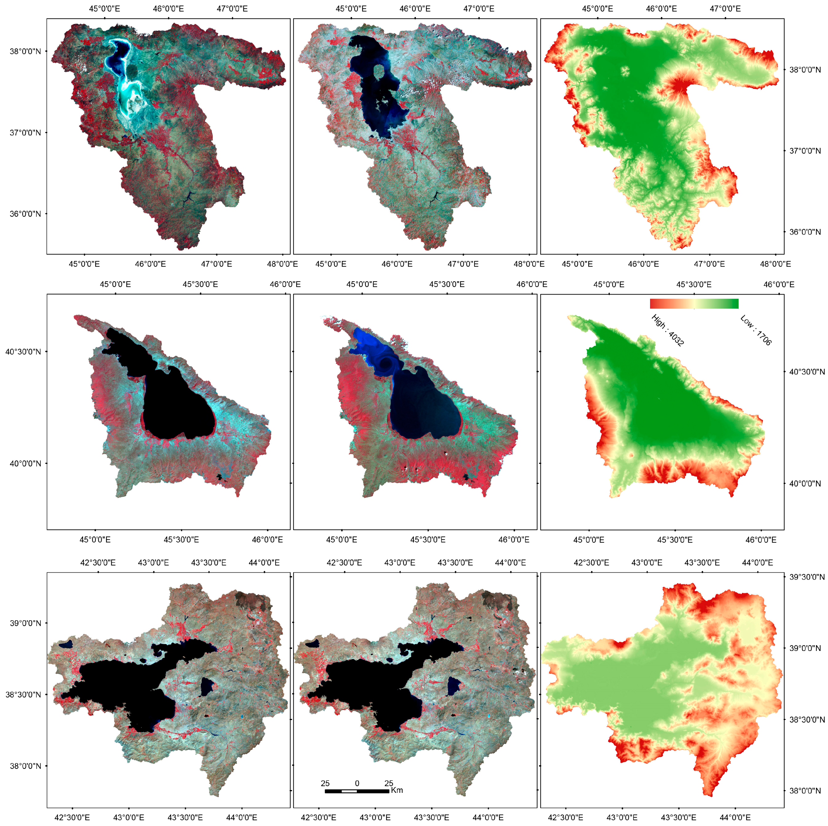
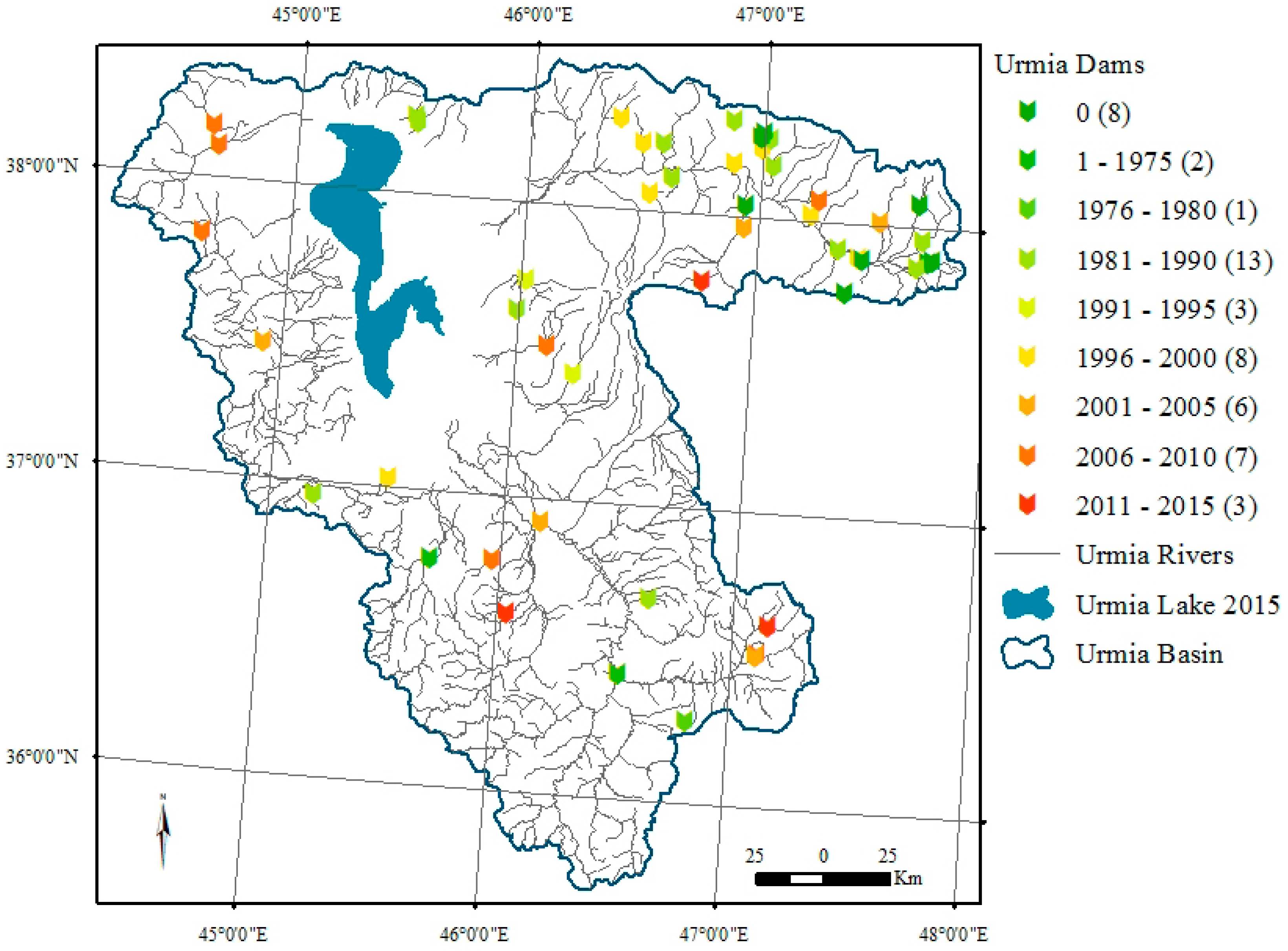
2.1. Urmia Lake
2.2. Lake Sevan
2.3. Van Lake
3. Data
3.1. Landsat and Digital Elevation Model (DEM) Dataset
3.2. Radar Altimetry Dataset
4. Methods and Algorithms
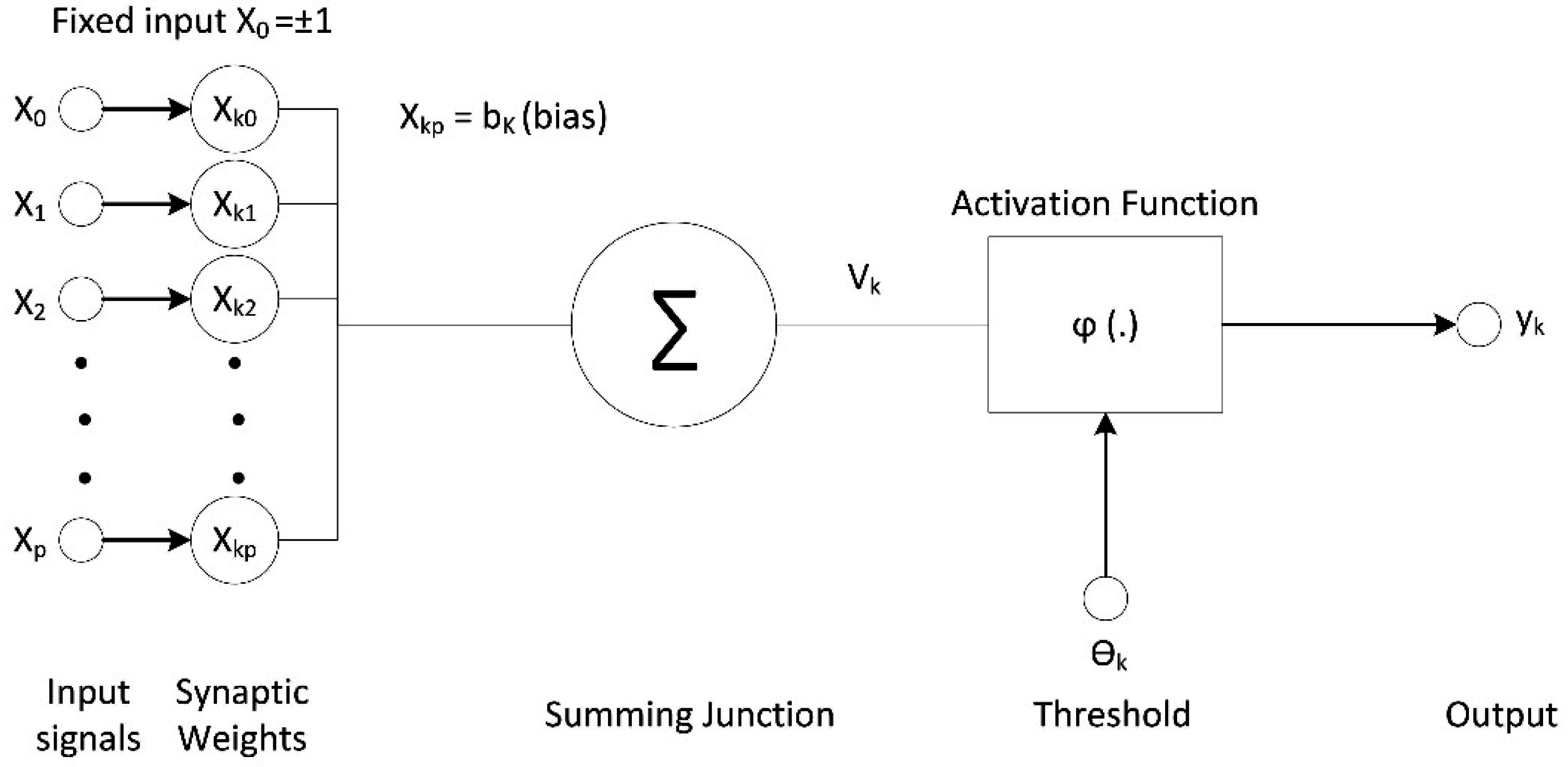
4.1. An Overview of MultiLayer Perceptron Neural Networks (MLP NNs)
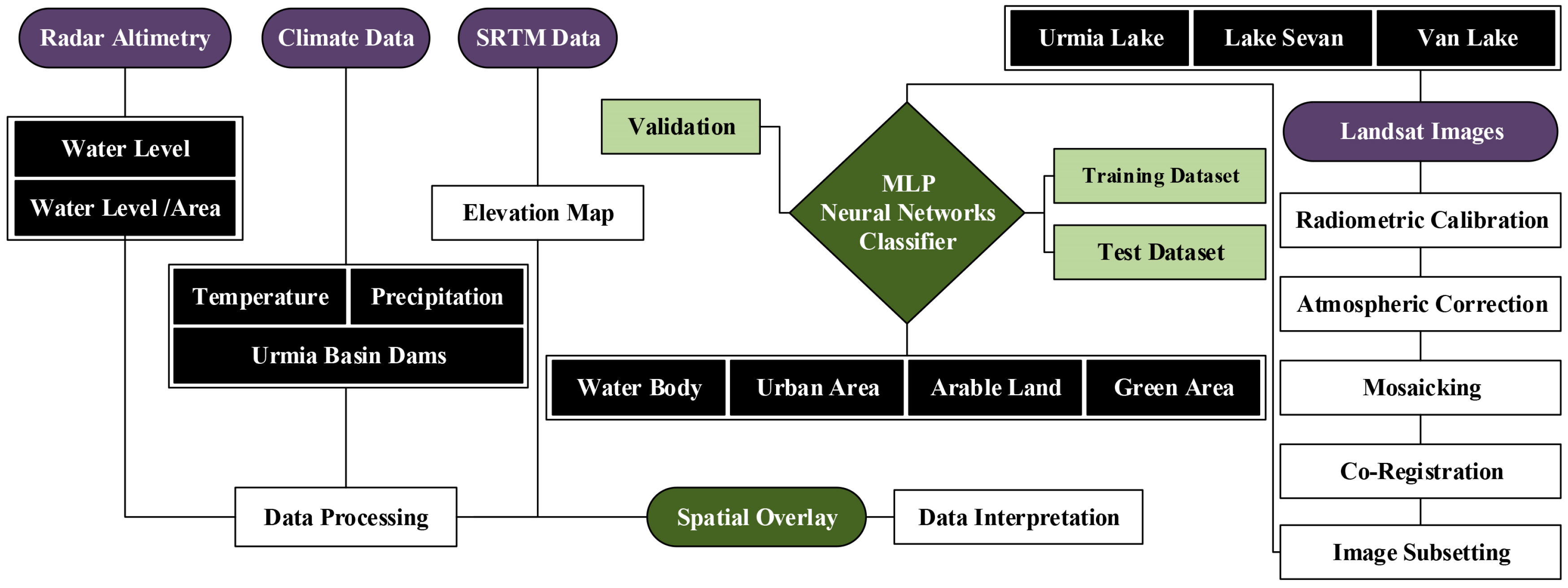
4.2. Methodology
4.2.1. Image Pre-Processing
4.2.2. Image Classification
4.2.3. Models Comparison
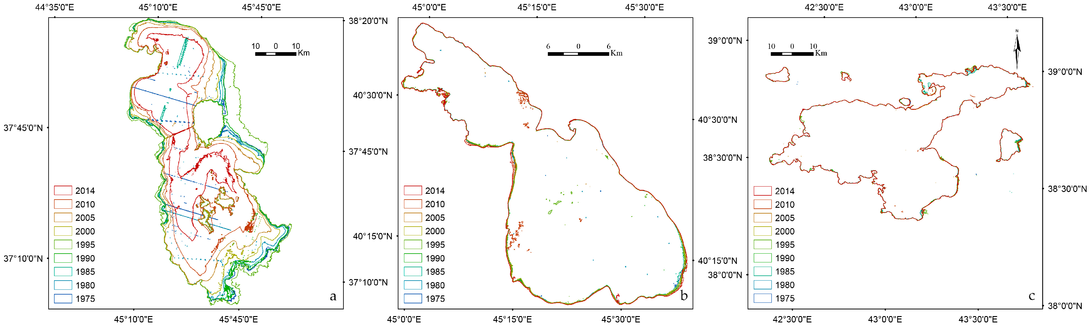
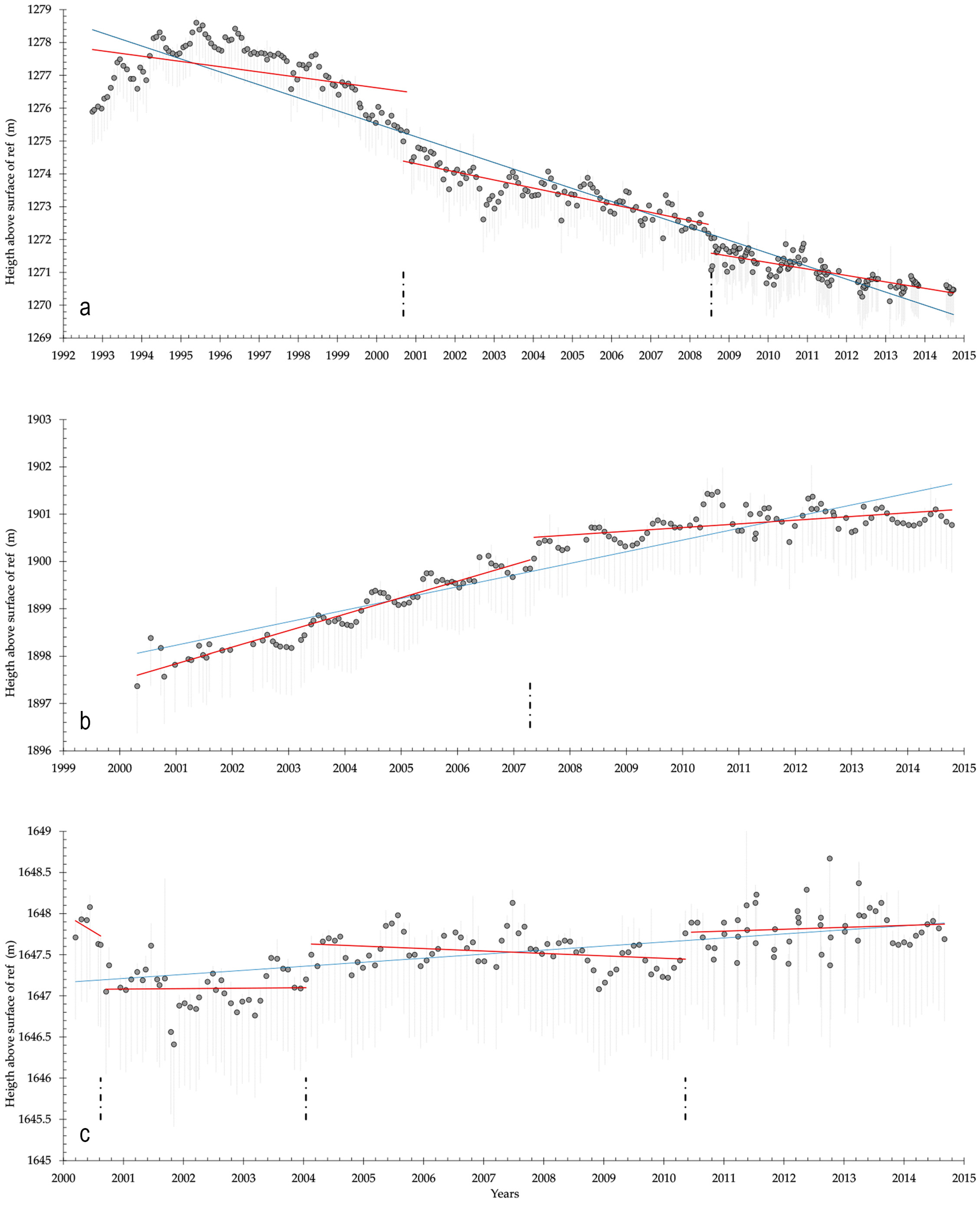
4.2.4. Time Series Change Detection
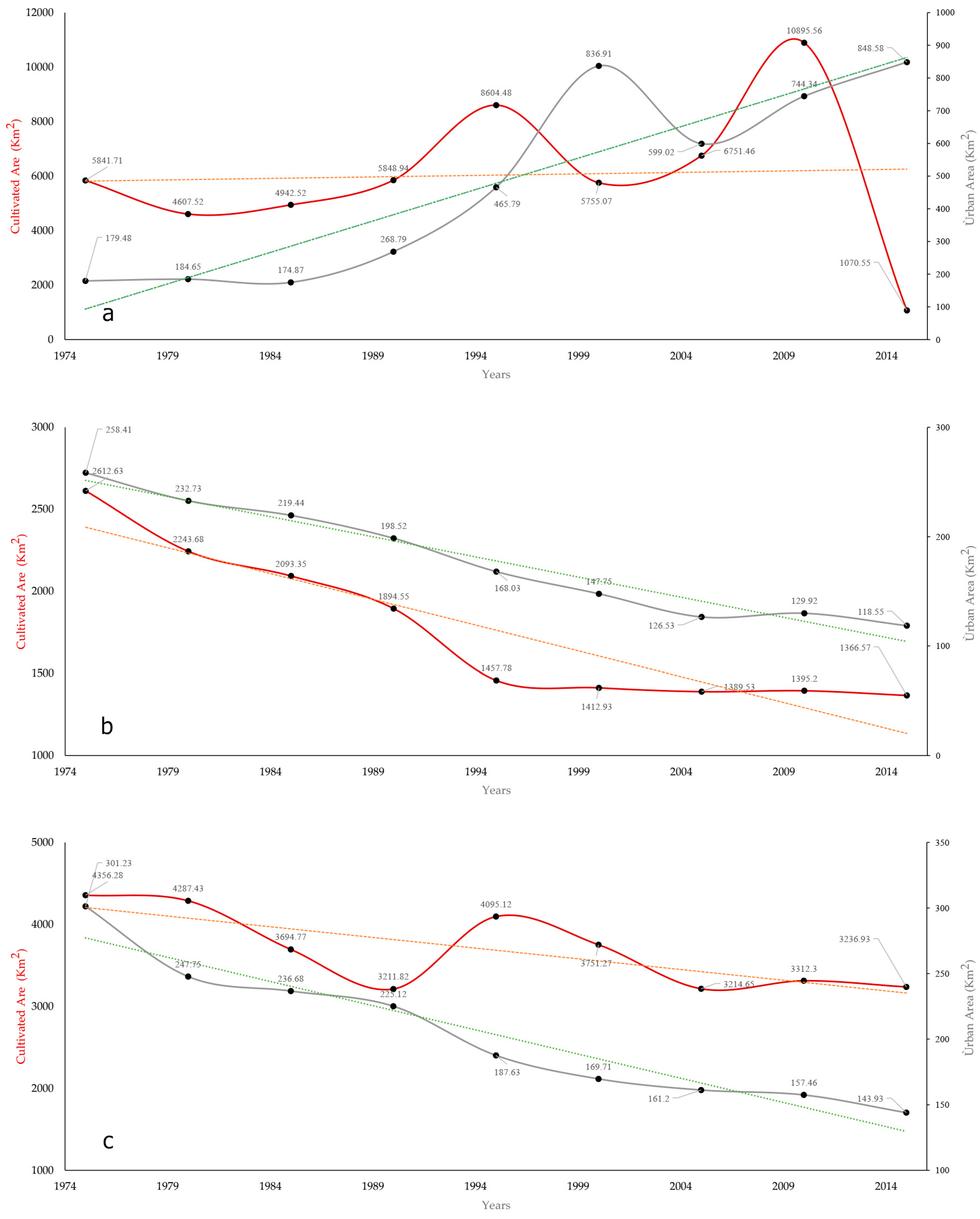
5. Results and Discussion
6. Conclusions
Acknowledgments
Author Contributions
Conflicts of Interest
References
- Zhu, W.; Jia, S.; Lv, A. Monitoring the fluctuation of Lake Qinghai using multi-source remote sensing data. Remote Sens. 2014, 6, 10457–10482. [Google Scholar] [CrossRef]
- Daily, G. Nature’s Services: Societal Dependence on Natural Ecosystems; Island Press: Washington, DC, USA, 1997; p. 329. [Google Scholar]
- Ozesmi, S.L.; Bauer, M.E. Satellite remote sensing of wetlands. Wetl. Ecol. Manag. 2002, 10, 381–402. [Google Scholar] [CrossRef]
- Crétaux, J.-F.; Jelinski, W.; Calmant, S.; Kouraev, A.; Vuglinski, V.; Bergé-Nguyen, M.; Gennero, M.-C.; Nino, F.; Del Rio, R.A.; Cazenave, A. Sols: A lake database to monitor in the near real time water level and storage variations from remote sensing data. Adv. Space Res. 2011, 47, 1497–1507. [Google Scholar] [CrossRef]
- Alsdorf, D.E.; Rodriguez, E.; Lettenmaier, D.P. Measuring surface water from space. Rev. Geophys. 2007, 45. [Google Scholar] [CrossRef]
- Calmant, S.; Seyler, F.; Cretaux, J.F. Monitoring continental surface waters by satellite altimetry. Surv. Geophys. 2008, 29, 247–269. [Google Scholar] [CrossRef]
- Frappart, F.; Calmant, S.; Cauhopé, M.; Seyler, F.; Cazenave, A. Preliminary results of ENVISAT RA-2-derived water levels validation over the Amazon basin. Remote Sens. Environ. 2006, 100, 252–264. [Google Scholar] [CrossRef] [Green Version]
- Duan, Z.; Bastiaanssen, W. Estimating water volume variations in lakes and reservoirs from four operational satellite altimetry databases and satellite imagery data. Remote Sens. Environ. 2013, 134, 403–416. [Google Scholar] [CrossRef]
- Medina, C.E.; Gomez-Enri, J.; Alonso, J.J.; Villares, P. Water level fluctuations derived from ENVISAT Radar Altimeter (RA-2) and in-situ measurements in a subtropical waterbody: Lake Izabal (Guatemala). Remote Sens. Environ. 2008, 112, 3604–3617. [Google Scholar] [CrossRef]
- Zhang, J.; Xu, K.; Yang, Y.; Qi, L.; Hayashi, S.; Watanabe, M. Measuring water storage fluctuations in Lake Dongting, China, by Topex/Poseidon satellite altimetry. Environ. Monit. Assess. 2006, 115, 23–37. [Google Scholar] [CrossRef] [PubMed]
- Crétaux, J.-F.; Birkett, C. Lake studies from satellite radar altimetry. C. R. Geosci. 2006, 338, 1098–1112. [Google Scholar] [CrossRef]
- Demir, B.; Bovolo, F.; Bruzzone, L. Updating land-cover maps by classification of image time series: A novel change-detection-driven transfer learning approach. IEEE Trans. Geosci. Remote Sens. 2013, 51, 300–312. [Google Scholar] [CrossRef]
- Salmon, B.P.; Kleynhans, W.; van den Bergh, F.; Olivier, J.C.; Grobler, T.L.; Wessels, K.J. Land cover change detection using the internal covariance matrix of the extended Kalman filter over multiple spectral bands. IEEE J. Sel. Top. Appl. Earth Obs. Remote Sens. 2013, 6, 1079–1085. [Google Scholar] [CrossRef]
- Brisco, B.; Schmitt, A.; Murnaghan, K.; Kaya, S.; Roth, A. SAR polarimetric change detection for flooded vegetation. Int. J. Digit. Earth 2013, 6, 103–114. [Google Scholar] [CrossRef]
- Volpi, M.; Petropoulos, G.P.; Kanevski, M. Flooding extent cartography with Landsat TM imagery and regularized kernel fisher’s discriminant analysis. Comput. Geosci. 2013, 57, 24–31. [Google Scholar] [CrossRef]
- Kaliraj, S.; Meenakshi, S.M.; Malar, V. Application of remote sensing in detection of forest cover changes using geo-statistical change detection matrices—A case study of Devanampatti reserve forest, Tamilnadu, India. Nat. Environ. Pollut. Technol. 2012, 11, 261–269. [Google Scholar]
- Markogianni, V.; Dimitriou, E.; Kalivas, D. Land-use and vegetation change detection in plastira artificial lake catchment (Greece) by using remote-sensing and GIS techniques. Int. J. Remote Sens. 2013, 34, 1265–1281. [Google Scholar] [CrossRef]
- Bagan, H.; Yamagata, Y. Landsat analysis of urban growth: How Tokyo became the world’s largest megacity during the last 40 years. Remote Sens. Environ. 2012, 127, 210–222. [Google Scholar] [CrossRef]
- Raja, R.A.; Anand, V.; Kumar, A.S.; Maithani, S.; Kumar, V.A. Wavelet based post classification change detection technique for urban growth monitoring. J. Indian Soc. Remote Sens. 2013, 41, 35–43. [Google Scholar] [CrossRef]
- Dronova, I.; Gong, P.; Wang, L. Object-based analysis and change detection of major wetland cover types and their classification uncertainty during the low water period at Poyang lake, China. Remote Sens. Environ. 2011, 115, 3220–3236. [Google Scholar] [CrossRef]
- Zhu, X.; Cao, J.; Dai, Y. A decision tree model for meteorological disasters grade evaluation of flood. In Proceedings of the 2011 Fourth International Joint Conference on Computational Sciences and Optimization (CSO), Kunming and Lijiang, China, 15–19 April 2011; IEEE: Piscataway, NJ, USA, 2011; pp. 916–919. [Google Scholar]
- Calvet, J.-C.; Wigneron, J.-P.; Walker, J.; Karbou, F.; Chanzy, A.; Albergel, C. Sensitivity of passive microwave observations to soil moisture and vegetation water content: L-band to w-band. IEEE Trans. Geosci. Remote Sens. 2011, 49, 1190–1199. [Google Scholar] [CrossRef]
- Desmet, P.; Govers, G. A GIS procedure for automatically calculating the USLE LS factor on topographically complex landscape units. J. Soil Water Conserv. 1996, 51, 427–433. [Google Scholar]
- Du, Z.; Linghu, B.; Ling, F.; Li, W.; Tian, W.; Wang, H.; Gui, Y.; Sun, B.; Zhang, X. Estimating surface water area changes using time-series Landsat data in the Qingjiang River Basin, China. J. Appl. Remote Sens. 2012, 6, 063609. [Google Scholar] [CrossRef]
- Sun, F.; Sun, W.; Chen, J.; Gong, P. Comparison and improvement of methods for identifying waterbodies in remotely sensed imagery. Int. J. Remote Sens. 2012, 33, 6854–6875. [Google Scholar] [CrossRef]
- Bai, J.; Chen, X.; Li, J.; Yang, L.; Fang, H. Changes in the area of inland lakes in arid regions of central Asia during the past 30 years. Environ. Monit. Assess. 2011, 178, 247–256. [Google Scholar] [CrossRef] [PubMed]
- Jawak, S.D.; Kulkarni, K.; Luis, A.J. A review on extraction of lakes from remotely sensed optical satellite data with a special focus on cryospheric lakes. Adv. Remote Sens. 2015, 4, 196–213. [Google Scholar] [CrossRef]
- Mason, I.; Guzkowska, M.; Rapley, C.; Street-Perrott, F. The response of lake levels and areas to climatic change. Clim. Chang. 1994, 27, 161–197. [Google Scholar] [CrossRef]
- Goerner, A.; Jolie, E.; Gloaguen, R. Non-climatic growth of the saline Lake Beseka, Main Ethiopian Rift. J. Arid Environ. 2009, 73, 287–295. [Google Scholar] [CrossRef]
- Mercier, F.; Cazenave, A.; Maheu, C. Interannual lake level fluctuations (1993–1999) in Africa from Topex/Poseidon: Connections with ocean–atmosphere interactions over the Indian Ocean. Glob. Planet. Chang. 2002, 32, 141–163. [Google Scholar] [CrossRef]
- Tourian, M.; Elmi, O.; Chen, Q.; Devaraju, B.; Roohi, S.; Sneeuw, N. A spaceborne multisensor approach to monitor the desiccation of Lake Urmia in Iran. Remote Sens. Environ. 2015, 156, 349–360. [Google Scholar] [CrossRef]
- Birkett, C. The contribution of topex/poseidon to the global monitoring of climatically sensitive lakes. J. Geophys. Res. Oceans 1995, 100, 25179–25204. [Google Scholar] [CrossRef]
- Frappart, F.; Seyler, F.; Martinez, J.-M.; Leon, J.G.; Cazenave, A. Floodplain water storage in the Negro river basin estimated from microwave remote sensing of inundation area and water levels. Remote Sens. Environ. 2005, 99, 387–399. [Google Scholar] [CrossRef] [Green Version]
- Baup, F.; Frappart, F.; Maubant, J. Combining high-resolution satellite images and altimetry to estimate the volume of small lakes. Hydrol. Earth Syst. Sci. 2014, 18, 2007–2020. [Google Scholar] [CrossRef]
- Frappart, F.; Papa, F.; Güntner, A.; Werth, S.; Da Silva, J.S.; Tomasella, J.; Seyler, F.; Prigent, C.; Rossow, W.B.; Calmant, S. Satellite-based estimates of groundwater storage variations in large drainage basins with extensive floodplains. Remote Sens. Environ. 2011, 115, 1588–1594. [Google Scholar] [CrossRef] [Green Version]
- Ramillien, G.; Frappart, F.; Seoane, L. Application of the regional water mass variations from grace satellite gravimetry to large-scale water management in Africa. Remote Sens. 2014, 6, 7379–7405. [Google Scholar] [CrossRef]
- Singh, A.; Seitz, F.; Schwatke, C. Inter-annual water storage changes in the Aral Sea from multi-mission satellite altimetry, optical remote sensing, and GRACE satellite gravimetry. Remote Sens. Environ. 2012, 123, 187–195. [Google Scholar] [CrossRef]
- Yan, L.-J.; Qi, W. Lakes in Tibetan Plateau extraction from remote sensing and their dynamic changes. Acta Geosci. Sin. 2012, 33, 65–74. [Google Scholar]
- Jensen, J.R. Remote Sensing of the Environment: An Earth Resource Perspective 2/e; Pearson Education: Delhi, India, 2009; pp. 15–17. [Google Scholar]
- Song, C.; Huang, B.; Ke, L. Modeling and analysis of lake water storage changes on the Tibetan Plateau using multi-mission satellite data. Remote Sens. Environ. 2013, 135, 25–35. [Google Scholar] [CrossRef]
- Rokni, K.; Ahmad, A.; Selamat, A.; Hazini, S. Water feature extraction and change detection using multitemporal Landsat imagery. Remote Sens. 2014, 6, 4173–4189. [Google Scholar] [CrossRef]
- Xu, H. Modification of normalised difference water index (NDWI) to enhance open water features in remotely sensed imagery. Int. J. Remote Sens. 2006, 27, 3025–3033. [Google Scholar] [CrossRef]
- Ouma, Y.O.; Tateishi, R. A water index for rapid mapping of shoreline changes of five East African Rift Valley lakes: An empirical analysis using Landsat TM and ETM+ data. Int. J. Remote Sens. 2006, 27, 3153–3181. [Google Scholar] [CrossRef]
- Frazier, P.S.; Page, K.J. Water body detection and delineation with Landsat TM data. Photogramm. Eng. Remote Sens. 2000, 66, 1461–1468. [Google Scholar]
- Soh, L.-K.; Tsatsoulis, C. Segmentation of satellite imagery of natural scenes using data mining. IEEE Trans. Geosci. Remote Sens. 1999, 37, 1086–1099. [Google Scholar]
- Alecu, C.; Oancea, S.; Bryant, E. Multi-resolution analysis of MODIS and ASTER satellite data for water classification. In Proceedings of the Remote Sensing for Environmental Monitoring, GIS Applications, and Geology, Bruges, Belgium, 19 September 2005; International Society for Optics and Photonics: Bellingham, WA, USA, 2005; p. 59831Z. [Google Scholar]
- Zhang, Y.; Pulliainen, J.T.; Koponen, S.S.; Hallikainen, M.T. Water quality retrievals from combined Landsat TM data and ERS-2 SAR data in the Gulf of Finland. IEEE Trans. Geosci. Remote Sens. 2003, 41, 622–629. [Google Scholar] [CrossRef]
- Yang, K.; Smith, L.C. Supraglacial streams on the Greenland ice sheet delineated from combined spectral–shape information in high-resolution satellite imagery. IEEE Geosci. Remote Sens. Lett. 2013, 10, 801–805. [Google Scholar] [CrossRef]
- Jawak, S.D.; Luis, A.J. Improved land cover mapping using high resolution multiangle 8-band WorldView-2 satellite remote sensing data. J. Appl. Remote Sens. 2013, 7, 073573. [Google Scholar] [CrossRef]
- Shao, P.; Yang, G.; Niu, X.; Zhang, X.; Zhan, F.; Tang, T. Information extraction of high-resolution remotely sensed image based on multiresolution segmentation. Sustainability 2014, 6, 5300–5310. [Google Scholar] [CrossRef]
- Jeon, Y.-J.; Choi, J.-G.; Kim, J.-I. A study on supervised classification of remote sensing satellite image by bayesian algorithm using average fuzzy intracluster distance. In International Workshop on Combinatorial Image Analysis; Klette, R., Žunić, J., Eds.; Springer: Berlin/Heidelberg, Germany, 2004; pp. 597–606. [Google Scholar]
- McFeeters, S.K. The use of the normalized difference water index (NDWI) in the delineation of open water features. Int. J. Remote Sens. 1996, 17, 1425–1432. [Google Scholar] [CrossRef]
- Shen, L.; Li, C. Water body extraction from Landsat ETM+ imagery using adaboost algorithm. In Proceedings of the 18th International Conference on Geoinformatics, Beijing, China, 18–20 June 2010; pp. 1–4.
- Rouse, J.W., Jr.; Haas, R.; Schell, J.; Deering, D. Monitoring vegetation systems in the Great Plains with ERTS. NASA Spec. Publ. 1974, 351, 309. [Google Scholar]
- Feyisa, G.L.; Meilby, H.; Fensholt, R.; Proud, S.R. Automated water extraction index: A new technique for surface water mapping using Landsat imagery. Remote Sens. Environ. 2014, 140, 23–35. [Google Scholar] [CrossRef]
- Feizizadeh, B.; Blaschke, T. GIS-multicriteria decision analysis for landslide susceptibility mapping: Comparing three methods for the Urmia Lake Basin, Iran. Nat. Hazards 2013, 65, 2105–2128. [Google Scholar] [CrossRef]
- AghaKouchak, A.; Norouzi, H.; Madani, K.; Mirchi, A.; Azarderakhsh, M.; Nazemi, A.; Nasrollahi, N.; Farahmand, A.; Mehran, A.; Hasanzadeh, E. Aral sea syndrome desiccates Lake Urmia: Call for action. J. Gt. Lakes Res. 2015, 41, 307–311. [Google Scholar] [CrossRef]
- Ghaheri, M.; Baghal-Vayjooee, M.; Naziri, J. Lake Urmia, Iran: A summary review. Int. J. Salt Lake Res. 1999, 8, 19–22. [Google Scholar] [CrossRef]
- Alipour, S. Hydrogeochemistry of seasonal variation of Urmia Salt Lake, Iran. Saline Syst. 2006, 2, 1448. [Google Scholar] [CrossRef] [PubMed]
- Centre, I.C. Iranian Cities Population. Available online: http://www.amar.org.ir (accessed on 3 October 2016).
- Ahmadzadeh Kokya, T.; Pejman, A.; Mahin Abdollahzadeh, E.; Ahmadzadeh Kokya, B.; Nazariha, M. Evaluation of salt effects on some thermodynamic properties of Urmia Lake water. I. J. Environ. Res. 2011, 5, 343–348. [Google Scholar]
- Hassanzadeh, E.; Zarghami, M.; Hassanzadeh, Y. Determining the main factors in declining the Urmia Lake level by using system dynamics modeling. Water Resour. Manag. 2012, 26, 129–145. [Google Scholar] [CrossRef]
- United Nations Environment Programme (UNEP); Global Environmental Alert Service (GEAS). The drying of Iran’s Lake Urmia and its environmental consequences. J. Environ. Dev. 2012, 2, 128–137. [Google Scholar]
- Birkett, C.M.; Mason, I.M. A new global lakes database for a remote sensing program studying climatically sensitive large lakes. J. Gt. Lakes Res. 1995, 21, 307–318. [Google Scholar] [CrossRef]
- Abbaspour, M.; Nazaridoust, A. Determination of environmental water requirements of Lake Urmia, Iran: An ecological approach. Int. J. Environ. Stud. 2007, 64, 161–169. [Google Scholar] [CrossRef]
- Alesheikh, A.A.; Ghorbanali, A.; Nouri, N. Coastline change detection using remote sensing. Int. J. Environ. Sci. Technol. 2007, 4, 61–66. [Google Scholar] [CrossRef]
- Feizizadeh, B.; Blaschke, T.; Nazmfar, H.; Rezaei Moghaddam, M. Landslide susceptibility mapping for the Urmia Lake Basin, Iran: A multi-criteria evaluation approach using GIS. Int. J. Environ. Res. 2013, 7, 319–336. [Google Scholar]
- Djamali, M.; de Beaulieu, J.-L.; Shah-Hosseini, M.; Andrieu-Ponel, V.; Ponel, P.; Amini, A.; Akhani, H.; Leroy, S.A.; Stevens, L.; Lahijani, H. A late pleistocene long pollen record from Lake Urmia, NW Iran. Quat. Res. 2008, 69, 413–420. [Google Scholar] [CrossRef]
- Sima, S.; Tajrishy, M. Using satellite data to extract volume–area–elevation relationships for Urmia Lake, Iran. J. Gt. Lakes Res. 2013, 39, 90–99. [Google Scholar] [CrossRef]
- Eimanifar, A.; Mohebbi, F. Urmia Lake (Northwest Iran): A brief review. Saline Syst. 2007, 3, 1–8. [Google Scholar] [CrossRef] [PubMed]
- Karbassi, A.; Bidhendi, G.N.; Pejman, A.; Bidhendi, M.E. Environmental impacts of desalination on the ecology of Lake Urmia. J. Gt. Lakes Res. 2010, 36, 419–424. [Google Scholar] [CrossRef]
- Faramarzi, N. Agricultural Water Use in Lake Urmia Basin, Iran: An Approach to Adaptive Policies and Transition to Sustainable Irrigation Water Use. Master’s Thesis, Uppsala University, Uppsala, Sweden, 2012. [Google Scholar]
- Babayan, A.; Hakobyan, S.; Jenderedjian, K.; Muradyan, S.; Voskanov, M. Lake Sevan: Experience and lessons learned brief. In Proceedings of the Lake Basin Management Initiative Regional Workshop for Europe, Central Asia and the Americas, Colchester, VT, USA, 18–21 June 2003; Available online: http://www.worldlakes.org/uploads/sevan_01oct2004.pdf (accessed on 21 October 2016).
- Enderedjian, K. Implementation of the Ramsay Strategic Plan in Management of Wetlands in Sevan National Park; Professional and Entrepreneurial Orientation Union: Yerevan-Sevan, Armenia, 2001; p. 125. [Google Scholar]
- Barseghyan, A. Wetland Vegetation of Armenian SSR; Academy of Sciences of Armenia: Yerevan, Armenia, 1990. [Google Scholar]
- Babayan, A.; Hakobyan, S.; Jenderedjian, K.; Muradyan, S.; Voskanov, M. Lake Sevan: Experience and lessons learned brief. In Lake Basin Management Initiative (LBMI); ILEC Foundation: Otsu, Japan, 2005; pp. 347–362. [Google Scholar]
- Agricultural Map of Armenian SSR; USSR: Moscow, Russia; Yerevan, Armenia, 1984; p. 189.
- Aksoy, H.; Unal, N.; Eris, E.; Yuce, M. Stochastic modeling of Lake Van water level time series with jumps and multiple trends. Hydrol. Earth Syst. Sci. 2013, 17, 2297–2303. [Google Scholar] [CrossRef]
- Wilkinson, I.P.; Gulakyan, S.Z. Holocene to Recent Ostracoda of Lake Sevan, Armenia: Biodiversity and ecological controls. Stratigraphy 2010, 7, 301–315. [Google Scholar]
- Thiel, V.; Jenisch, A.; Landmann, G.; Reimer, A.; Michaelis, W. Unusual distributions of long-chain alkenones and tetrahymanol from the highly alkaline Lake Van, Turkey. Geochim. Cosmochim. Acta 1997, 61, 2053–2064. [Google Scholar] [CrossRef]
- Stockhecke, M.; Anselmetti, F.S.; Meydan, A.F.; Odermatt, D.; Sturm, M. The annual particle cycle in Lake Van (Turkey). Palaeogeogr. Palaeoclim. Palaeoecol. 2012, 333, 148–159. [Google Scholar] [CrossRef]
- Roberts, N.; Wright, H., Jr. Vegetational, lake-level, and climatic history of the Near East and Southwest Asia. In Global Climates Since the Last Glacial Maximum; University of Minnesota Press: Minneapolis, MN, USA, 1993; pp. 194–220. [Google Scholar]
- Warren, J.K. Evaporites: Sediments, Resources and Hydrocarbons; Springer Science & Business Media: Berlin, Germany, 2006. [Google Scholar]
- Wick, L.; Lemcke, G.; Sturm, M. Evidence of Lateglacial and Holocene climatic change and human impact in eastern Anatolia: High-resolution pollen, charcoal, isotopic and geochemical records from the laminated sediments of Lake Van, Turkey. Holocene 2003, 13, 665–675. [Google Scholar] [CrossRef]
- Coskun, M.; Musaoglu, N. Investigation of rainfall-runoff modelling of the van lake catchment by using remote sensing and GIS integration. In International Archives of Photogrammetry Remote Sensing and Spatial Information Sciences, Proceedings of the XXth ISPRS Congress, Commission VII, Istanbul, Turkey, 12–23 July 2004; ISPRS: Istanbul, Turkey, 2004; pp. 12–23. [Google Scholar]
- Aladin, N.; Crétaux, J.F.; Plotnikov, I.; Kouraev, A.; Smurov, A.; Cazenave, A.; Egorov, A.; Papa, F. Modern hydro-biological state of the Small Aral Sea. Environmetrics 2005, 16, 375–392. [Google Scholar] [CrossRef]
- Cretaux, J.-F.; Kuraev, A.A.V.; Papa, F.; Nguyen, M.B.; Cazenave, A.; Aladin, N.V.; Plotnikov, I.S. Water balance of the Big Aral Sea from satellite remote sensing and in situ observations. J. Gt. Lakes Res. 2005, 31, 520–534. [Google Scholar] [CrossRef]
- Theia-Land. Hydroweb. Available online: http://hydroweb.theia-land.fr (accessed on 19 October 2016).
- Fernandes, D. Segmentation of SAR images with Weibull distribution. In Proceedings of the Geoscience and Remote Sensing Symposium, IGARSS’98, Seattle, WA, USA, 6–10 July 1998; pp. 24–26.
- Bishop, C.M. Neural Networks for Pattern Recognition; Oxford University Press: Oxford, UK, 1995. [Google Scholar]
- Taravat, A.; Del Frate, F.; Cornaro, C.; Vergari, S. Neural networks and support vector machine algorithms for automatic cloud classification of whole-sky ground-based images. IEEE Geosci. Remote Sens. Lett. 2015, 12, 666–670. [Google Scholar] [CrossRef]
- Schroeder, T.A.; Cohen, W.B.; Song, C.; Canty, M.J.; Yang, Z. Radiometric correction of multi-temporal Landsat data for characterization of early successional forest patterns in western Oregon. Remote Sens. Environ. 2006, 103, 16–26. [Google Scholar] [CrossRef]
- Taravat, A.; Del Frate, F. Development of band ratioing algorithms and neural networks to detection of oil spills using Landsat ETM+ data. EURASIP J. Adv. Signal Process. 2012, 2012, 1–8. [Google Scholar] [CrossRef]
- Bishop, C.M. Pattern Recognition and Machine Learning; Springer: New York, NY, USA, 2006. [Google Scholar]
- Jackson, B.; Scargle, J.D.; Barnes, D.; Arabhi, S.; Alt, A.; Gioumousis, P.; Gwin, E.; Sangtrakulcharoen, P.; Tan, L.; Tsai, T.T. An algorithm for optimal partitioning of data on an interval. IEEE Signal Process. Lett. 2005, 12, 105–108. [Google Scholar] [CrossRef]
- Killick, R.; Fearnhead, P.; Eckley, I. Optimal detection of changepoints with a linear computational cost. J. Am. Stat. Assoc. 2012, 107, 1590–1598. [Google Scholar] [CrossRef]


| MinOm | MaxOm | MeanOm | St.DevOm | MinCm | MaxCm | MeanCm | St.DevCm | |
|---|---|---|---|---|---|---|---|---|
| MNDWI | 13.60 | 26.80 | 23.69 | 3.75 | 17.60 | 25.50 | 15.02 | 3.09 |
| AWEI | 12.60 | 28.50 | 20.79 | 4.02 | 9.70 | 22.10 | 12.33 | 2.94 |
| NDVI | 10.80 | 30.00 | 20.28 | 5.26 | 9.30 | 30.39 | 14.95 | 6.16 |
| NDWI | 13.80 | 21.30 | 17.03 | 2.69 | 3.40 | 10.80 | 7.27 | 2.93 |
| WRI | 14.00 | 22.00 | 18.68 | 2.26 | 5.30 | 10.8 | 7.89 | 2.11 |
| NDWI-PCs | 10.80 | 18.00 | 13.90 | 2.47 | 4.50 | 10.80 | 7.67 | 2.36 |
| MLP ANNs | 2.50 | 10.00 | 4.47 | 2.00 | 1.40 | 8.50 | 3.88 | 2.19 |
| Min % | Max % | Mean % | St.Dev | |
|---|---|---|---|---|
| MNDWI | 73.20 | 86.40 | 76.33 | 3.73 |
| AWEI | 71.50 | 87.40 | 79.20 | 4.20 |
| NDVI | 70.00 | 89.20 | 79.71 | 5.27 |
| NDWI | 78.70 | 86.20 | 82.96 | 2.69 |
| WRI | 78.00 | 86.00 | 81.31 | 2.26 |
| NDWI-PCs | 82.00 | 89.20 | 86.10 | 2.47 |
| MLP ANNs | 90.00 | 97.50 | 95.52 | 2.00 |
| Urmia Lake Surface Area | Lake Sevan Surface Area | Van Lake Surface Area | |
|---|---|---|---|
| 1975 | 5235.85 | 1259.52 | 3751.22 |
| 1980 | 4977.71 | 1255.95 | 3749.84 |
| 1985 | 5132.71 | 1246.02 | 3743.85 |
| 1990 | 5214.18 | 1231.33 | 3727.70 |
| 1995 | 5821.82 | 1236.03 | 3768.73 |
| 2000 | 4724.69 | 1234.77 | 3738.77 |
| 2005 | 4111.12 | 1226.04 | 3691.45 |
| 2010 | 3184.73 | 1236.74 | 3726.48 |
| 2015 | 1642.71 | 1230.15 | 3716.44 |
© 2016 by the authors; licensee MDPI, Basel, Switzerland. This article is an open access article distributed under the terms and conditions of the Creative Commons Attribution (CC-BY) license (http://creativecommons.org/licenses/by/4.0/).
Share and Cite
Taravat, A.; Rajaei, M.; Emadodin, I.; Hasheminejad, H.; Mousavian, R.; Biniyaz, E. A Spaceborne Multisensory, Multitemporal Approach to Monitor Water Level and Storage Variations of Lakes. Water 2016, 8, 478. https://doi.org/10.3390/w8110478
Taravat A, Rajaei M, Emadodin I, Hasheminejad H, Mousavian R, Biniyaz E. A Spaceborne Multisensory, Multitemporal Approach to Monitor Water Level and Storage Variations of Lakes. Water. 2016; 8(11):478. https://doi.org/10.3390/w8110478
Chicago/Turabian StyleTaravat, Alireza, Masih Rajaei, Iraj Emadodin, Hamidreza Hasheminejad, Rahman Mousavian, and Ehsan Biniyaz. 2016. "A Spaceborne Multisensory, Multitemporal Approach to Monitor Water Level and Storage Variations of Lakes" Water 8, no. 11: 478. https://doi.org/10.3390/w8110478