Assessment of FAO AquaCrop Model for Simulating Maize Growth and Productivity under Deficit Irrigation in a Tropical Environment

Abstract

Crop simulation models have a pivotal role to play in evaluating irrigation management strategies for improving agricultural water use. The objective of this study was to test and validate the AquaCrop model for maize under deficit irrigation management. Field observations from three experiments consisting of four treatments were used to evaluate model performance in simulating canopy cover (CC), biomass (B), yield (Y), crop evapotranspiration (ET_c), and water use efficiency (WUE). Statistics for root mean square error, model efficiency (E), and index of agreement for B and CC suggest that the model prediction is good under non-stressed and moderate stress environments. Prediction of final B and Y under these conditions was acceptable, as indicated by the high coefficient of determination and deviations <10%. In severely stressed conditions, low E and deviations >11% for B and 9% for Y indicate a reduction in the model reliability. Simulated ET_c and WUE deviation from observed values were within the range of 9.5% to 22.2% and 6.0% to 32.2%, respectively, suggesting that AquaCrop prediction of these variables is fair, becoming unsatisfactory as plant water stress intensifies. AquaCrop can be reliably used for evaluating the effectiveness of proposed irrigation management strategies for maize; however, the limitations should be kept in mind when interpreting the results in severely stressed conditions.

1. Introduction

Population growth, land use change, climate change, and increasing demand in non-agricultural sectors profoundly affect the availability and quality of water resources for irrigated agriculture. Amid increasing concerns that water scarcity and food security are among the main problems to be faced by many societies in the 21st century, a global challenge for the agricultural sector is to produce more food with less water [1]. Irrigation strategies focusing on increasing agricultural water productivity, such as deficit irrigation (DI) coupled with crop simulation modeling to investigate multiple alternatives, have a pivotal role to play in sustainable water development.

Extensive research and publications highlight the contribution DI management strategy makes in combating water waste in irrigation. By providing less than the exact crop water requirements, specifically during drought-tolerant growth stages, crop yields can be stabilized and maximum water use efficiency (WUE) attained [2]. Judicious planning is therefore required as supplying crops with less than their water requirement can significantly affect crop growth and development, inevitably affecting yield, especially if water stress occurs during the susceptible growth stage. DI is a flexible management strategy and its successful implementation is dependent on a sound irrigation schedule, in terms of both timing and application amount. Therefore, there exist numerous possibilities when investigating and imposing a DI management plan. Some of these include growth-stage-specific DI, intermittent DI (irrigation is applied on specific days), and root zone soil moisture depletion. In each case, different water amounts can be applied. Owing to their cost and time effectiveness, crop simulation models are ideally suited for the evaluation of irrigation strategies where there are various alternatives.

The FAO AquaCrop simulation model provides a sound theoretical framework to investigate crop yield response to environmental stress [3]. This model has successfully simulated crop growth and yield as influenced by varying soil moisture environments for crops like sunflower [4], bambara groundnut [5], and winter wheat [6]. Farahani et al. [3] and Geerts et al. [7] suggest that this model maintains a good balance between robustness and accuracy, and a noteworthy feature of the model compared to other cereal crop growth models is the simplicity it offers its users; it does not require advanced skill for its calibration or operation and does not require a large number of input parameters [8]. The relatively small number of input data describes the soil–crop–atmosphere environment in which the crop develops, most of which can be derived by simple methods. AquaCrop simulates crop growth and yield based on the water-driven growth model that relies on the conservative behavior of biomass per unit transpiration relationship [4,9]. This fundamental principle contributed to the simplistic structure of the model, having a greater applicability in space and time, as the model features “conservative input parameters” that transcend geographical location and cultivar [9,10]. Raes et al. [11] noted that these conservative parameters require no adjustment to the localized environments, favorable or limiting conditions, as their modulation is triggered by stress response functions.

AquaCrop yield response model has been applied to a wide range of crops including maize. Heng et al. [8] and Hsiao et al. [12] reported that AquaCrop simulated maize development, grain yield, and water variables such as the crop evapotranspiration (ET_c) and WUE, to name a few, reasonably well in cases of non-limiting conditions. Still, some studies report that model performance declines in estimating some variables in severe water stress environments [1,13]. Although a highlighted feature of the model is the applicability of conservative parameters used in crop simulations (these parameters are reported by Heng et al. [8] and Hsiao et al. [12] for maize), several researchers observed that model parameterization is essentially site-specific and that important calibrated parameters necessary for accurate simulation must be tested under different climate, soil, cultivars, irrigation methods, and field management to improve the reliability of the simulated results [3,14,15].

Owing to the diversification of its uses, maize is a cereal crop that significantly contributes to a country’s self-sufficiency. Taiwan has recorded a considerable decrease in maize production and now relies heavily on imports from the international market to meet demand [16]; the average cultivated area of maize in Taiwan is approximately 18,000 ha/year (2005–2009 estimate) from about 90,000 ha/year in 1980–1990 [17]. Amid a water-intensive rice industry (Taiwan’s main crop), the successful revival and planned expansion of maize production requires sustainable water management strategies, especially considering that dry spells are a characteristic feature of the main cropping season. The availability of a model adapted to local conditions should have a strong impact on planned expansions and would aid in assessing competing management alternatives and possible constraints. Integrating crop models that simulate the effects of water on crop yield with targeted experimentation can facilitate the development of irrigation strategies for high yield procurement and improving farm level water management and WUE.

The objectives of this research were two-fold: (1) To analyze the performance of AquaCrop for maize under full and deficit irrigation in the tropical environment of Southern Taiwan; and (2) to test and validate the effectiveness of the calibrated model in simulating biomass yield and grain yield under contrasting environmental conditions.

2. Materials and Methods

2.1. Field Experiments

2.1.1. Site Characteristics and Management Practices

Field experiments were conducted at the irrigation experimental site of National Pingtung University of Science and Technology, Southern Taiwan (22.65° N: 34.95° E: 71 m above sea level) for three cropping seasons. The climate of the study area is classified as tropical wet and dry with extreme spatial and temporal rainfall distribution. Two experiments were conducted during the main growing period running from November to March for 2014 to 2015 (Experiment 1) and 2015 to 2016 (Experiment 3). Another experiment was conducted during the summer season running from April to July of 2015 (Experiment 2). Utilizing the model for two distinct cropping seasons allows for better testing and evaluation of its effectiveness given the extreme spatial and temporal rainfall distribution of the study location. The late cropping season (November to March), one of the main cropping periods for maize, coincides with the cooler winter season and is characterized by warm dry spells and lack of rainfall. The other cropping season (April to July) coincides with the hot and humid summer months and typhoon season, which is characterized by intense and or long rainfall events that often lead to extensive damage to crops.

Weather data, including daily values of air temperature, humidity, wind speed (at 2 m height), solar radiation, and precipitation, were collected from an on-site agro-meteorological station. The two experiments occurring during the main growing months (November to March) had similar air temperature environments, with a seasonal mean of approximately 20 °C. During these periods, the mean daily maximum temperature ranged from 11 to 32 °C, while the mean daily minimum temperature ranged from 5 to 22 °C. On the other hand, the mean maximum temperature for Experiment 2 was consistently over 32 °C, with a seasonal mean of 28.7 °C. There was substantial difference in rainfall between the seasons. During Experiments 1 and 3 a total rainfall of 40 mm and 213.5 mm was recorded, respectively. The rainfall during Experiment 3 was atypical to that observed at the location; total long-term (15 years) rainfall during the cropping period averages 65.4 mm. In contrast, the total rainfall recorded during Experiment 2 was 890.5 mm, most of which was concentrated in two major events (Figure 1). The uneven distribution of rainfall affected the irrigation application (subsequently discussed). Cumulative reference evapotranspiration (ET_o), calculated via the FAO Penman–Monteith method as described in Allen et al. [18], was 286.3, 415.9, and 274.4 mm for Experiments 1, 2, and 3, respectively.

The soil at the experimental site is classified as loamy, with an average bulk density of 1.4 g·cm⁻³. The average volumetric water contents for a 1 m soil profile depth at saturation, field capacity, and permanent wilting point are 42.9%, 30.5%, and 15%, respectively.

Table 1. Some soil physical properties of the experimental site and initial soil water content (SWC) for the three experiments (Exp.) at different soil profile depths.

Soil Depth (m)	Field Capacity (m3·m−3)	Permanent Wilting Point (m3·m−3)	Initial SWC (% Volume)
			Exp. 1	Exp. 2	Exp. 3
0–0.2	0.305	0.150	28.1	21.1	26.1
0.2–0.4	0.299	0.143	31.2	22.3	25.7
0.4–0.6	0.304	0.151	29.6	26.6	27.1
0.6–0.8	0.310	0.159	30.8	25.7	26.7
0.8–1.0	0.312	0.148	31.7	28.0	29.1

shows important soil physical characteristics of the experimental site. During the three experiments, crops were subjected to the same field management practices. There were a total of 12 plots of 10 m², manually prepared with well-leveled basins. To avoid border and interaction effects, levees 0.30 m high and 1 m wide were created around the perimeter of each plot as buffer. Fertilizer was applied over the entire field when needed so that plants would not be subjected to nutrient stress. Insects and diseases were rigorously controlled during the cropping season and plots were hand weeded when necessary so that there was no competition for light, nutrients, or water.

2.1.2. Irrigation Treatments

The experiments for all seasons consisted of four irrigation treatments, replicated three times, arranged in a completely randomized block design. The treatment variation was based only on the amount of irrigated water applied, irrespective of the corn phenological growth stage. The rationale for this was to maintain a consistent irrigation schedule based on soil moisture content. It was hypothesized that this would vary the severity of the water stress levels. The four irrigation levels included a full irrigation treatment (FIT) and three deficit treatments corresponding to 67%, 50%, and 33% of water applied in the FIT. Irrigation depth was determined based on the concept of maximum allowable depletion of total available soil water (TAW) in the soil profile [19]. Using Equation (1) [19], the water applied to the FIT at each irrigation event was 60 mm. Subsequently, irrigation levels assigned to deficit treatments 67% FIT, 50% FIT, and 33% FIT was 40, 30, and 20 mm of water, respectively.

$$V_d=\frac{AD(\%)\left(FC-WP\right)R_{z}A}{100},$$

(1)

where V_d is the volume of irrigation water (m³), AD is the allowed depletion (40%) [20], FC is the field capacity (m³·m⁻³), WP is the permanent wilting point (m³·m⁻³), R_z is the effective rooting depth (1 m), and A is the surface area of the plot (m²). During early vegetative growth (VE to end of V5), all treatments received approximately 60–75 mm of water to establish plants and promote robust root development. Treatment management of irrigation water application thus began from the V6 growth stage, and it is here that the distinction was made in terms of 67%, 50%, and 33% FIT water applied. Given the temporal distribution of rainfall, the number of irrigation events in each season varied (Figure 1). There were a total of eight, four, and five irrigation events in Experiments 1, 2, and 3, respectively. Total water applied, which is equal to the sum of the initial amounts of water applied for plant establishment and the amount under the treatment management, to the different treatments in each season is presented in

Table 2. Timeline of main phenological growth stages in days after planting (DAP) and seasonal water applied for the different treatments for the three experiments (Exp.).

Agronomic Details	Growing Season
	Exp. 1	Exp. 2	Exp. 3
Planting density (plants m−2)	8.3	8.3	8.3
Sowing date	22 November	19 April	21 November
Emergence (DAP)	6	7	7
Anthesis (DAP)	60	54	71
Maturity (DAP)	114	99	120
Total Irrigation Water Applied (mm)
FIT	555 (480, 75) 1	300 (240, 60)	375 (300, 75)
67% FIT	395 (320, 75)	220 (160, 60)	275 (200, 75)
50% FIT	315 (240, 75)	180 (120, 60)	225 (150, 75)
33% FIT	235 (160, 75)	140 (80, 60)	175 (100, 75)

Note: ¹ Values in parentheses show the amount under irrigation treatment management and initial water applied for plant establishment.

. Flood irrigation by the use of carefully constructed water pipes and water meters was used to administer the required water depth to each treatment. Irrigation was initiated for all treatments whenever the soil moisture in the FIT was depleted by 40%. That is, in the deficit-irrigated treatments irrigation occurred on the same day as the fully irrigated plots, but the duration of irrigation applications were reduced to 67%, 50%, and 33% of the full irrigation. The 40% depletion criterion used for irrigation scheduling was determined by constantly monitoring the soil water status. The percentage depletion of available soil water in the effective root zone was estimated as follows [21]:

$$\mathrm{depletion}(\%)=100\times \frac{1}{n}{{\displaystyle \sum }}_1^n\frac{F{C}_i-{\mathsf{\theta }}_i}{F{C}_i-WP},$$

(2)

where n is the number of sub-divisions of the effective rooting depth used in the soil moisture sampling, FC_i is the soil moisture at field capacity for ith layer, θ_i is the soil moisture in ith layer, and WP is the soil moisture at permanent wilting point. θ was monitored daily using soil moisture sensors, EnviroScan system (Sentek Technologies, Stepney, Australia), connected to an automatic datalogger. Sensors were installed in between two plants on the same row through Sentek customized polyvinyl chloride (PVC) access tubes in two replicates per treatment. Daily soil water in the root zone was computed as the average of all 10-min interval readings for that day for the respective soil profile depths.

2.2. Data Collection and Measurements

The main phenological growth stages in days after planting (DAP) are presented in Table 2. To assess crop development, leaf area index (LAI) and total aboveground biomass were monitored throughout the cropping season. During Experiment 1, data was collected at regular three-week intervals from sowing to harvest, while collection was done approximately every two weeks during Experiment 3. For Experiment 2, extreme weather conditions resulted in severe damage to some plants and data collection of seasonal evolution of biomass and LAI had to be abandoned. To evaluate biomass accumulation, four plants per plot were randomly selected, clipped at the soil surface, then oven dried at 70 °C until constant weight was attained. At harvest, final grain yield and total oven-dry biomass per treatment were measured. Eight randomly selected plants per plot were tagged to monitor LAI throughout the growing season. The LAI was calculated as the product of the manually measured leaf area (maximal length x width) of each leaf, by the shape factor (k = 0.75) for maize, by the plant density [22]. LAI was converted to green canopy cover (CC) using Equation (3) [8,12]:

$$CC=1.005{\left[1-\exp \left(-0.6\mathrm{LAI}\right)\right]}^{1.2}.$$

(3)

The actual crop evapotranspiration (ET_c) of each treatment was calculated using the soil water balance method:

$$E{T}_{\mathrm{c}}=P+I-D-R\pm \Delta W,$$

(4)

where P is the rainfall (mm), I is the irrigation (mm), D is the downward drainage out of the root zone (mm), R is the surface runoff (mm), and $\Delta W$ is the change in the soil water content (SWC) (mm). R was assumed to be zero because irrigation water application was controlled and the experimental plots were enclosed by 1 m wide levees around the perimeter with basins meticulously prepared to be level. In Experiments 1 and 3, the SWC in the root zone was recorded using EnviroScan probes throughout the season from 0 to 1 m depth with 0.1 m intervals, and 1 to 1.6 m depth at 0.2 m intervals. The latter was used to observe drainage, as the effective root zone considered was 1 m. However, during Experiment 2 all SWC was measured on a weekly basis gravimetrically. Here, the SWC was monitored at 0.10-m intervals to a depth of 1 m and at 0.20 m intervals from 1 to 2 m soil profile depth. Field initial SWC (Table 1) was measured at sowing gravimetrically to ensure the accuracy of the sensors and for AquaCrop model input data.

2.3. Description of AquaCrop Simulation Model

2.3.1. Model Background

The AquaCrop model evolved from the Doorenbos and Kassam [23] Ky approach of modeling yield response to water. As outlined in Steduto et al. [9] and Raes et al. [11], there are two fundamental principles that separate this water-driven “growth engine” from its predecessor and other cropping models. First, the model simulates the separation of actual ET into soil evaporation and crop transpiration, thereby avoiding the confounding effect of the non-productive consumptive use of water. In addition, another distinguishing attribute of AquaCrop is that it uses green CC to express foliage development instead of LAI. The CC and ET_o are then used with the crop coefficient for transpiration to calculate transpiration for non-stress conditions, and with the soil evaporation coefficient to calculate soil evaporation each day [8]. Secondly, the model simulates the separation of yield into biomass and harvest index (HI). Crop yield is simulated as the product of biomass and HI. In AquaCrop, HI is identified as a conservative parameter, although the default value can be changed for a specific species or location. Additionally, HI is continuously adjusted in AquaCrop during yield formation in response to water and/or temperature stresses. AquaCrop estimates daily biomass production as follows:

$$B_i=W{P}^{*}{{\displaystyle \sum }}^{\text{}}\left(\frac{T{r}_i}{E{T}_{\mathrm{o}i}}\right),$$

(5)

where B_i is the daily aboveground biomass, Tr_i is the daily crop transpiration, $E{T}_{\mathrm{o}i}$ is the daily reference evapotranspiration, and WP* is the water productivity of the crop species normalized for both evaporative demand and atmospheric CO₂. The normalization of WP for climate makes AquaCrop applicable to diverse locations and seasons, including future climate scenarios [5].

In addition to crop growth, development, and yield production, AquaCrop simulates changes in the amount of water stored in the root zone by performing a daily water balance that includes all the incoming and outgoing water fluxes (infiltration, runoff, deep percolation, evaporation, and transpiration). In the model, there are four water stress response coefficients, which are functions of the fractional depletion of the total available water in the root zone used to express the effects of water deficit on the crop. The four coefficients are for leaf growth/canopy expansion, stomatal conductance, canopy senescence, and pollination failure/HI, each with its own threshold depletion level and response curves.

2.3.2. Parameters and Input Data

As in other crop models, AquaCrop consists of a soil–crop–atmosphere continuum. The climate component requires daily weather data on maximum and minimum air temperature, rainfall, ET_o, and CO₂ concentration. These data were collected from an agro-meteorological station located at the experimental site. Daily ET_o was calculated using the FAO Penman–Monteith equation.

The soil profile file requires basic soil characteristics such as volumetric water content at saturation, field capacity, permanent wilting point, and saturated hydraulic conductivity of the different soil profile depths. These parameters were obtained in accordance with standard international procedures. Groundwater effects through capillary action were not simulated as the groundwater table is well below the effective root zone (typically >7 m). Data required for the initial conditions file in AquaCrop was measured at the start of each experiment (Table 1). The input data also include information relating to the irrigation and field management. In general, these input parameters are location- and management-specific, and the necessary data were entered into the model as practiced in the field experiments.

The crop input component of AquaCrop contains both user-specific and conservative parameters, which can be categorized into crop parameters, phenology, development, and water stress groups. Some of the user-specific parameters include plant density, emergence time, canopy senescence and maturity time, flowering period and yield formation duration, rooting depth, and reference HI (may also be conservative). To name a few, some of the conservative crop parameters include soil water extraction pattern; canopy growth, given as a percentage of canopy cover; WP* for biomass; crop coefficient for transpiration at full canopy; and water stress response coefficients for canopy expansion, stomatal closure, and early canopy senescence. Given one of the experimental periods was during the rainy season when water logging is common, aeration stress was considered in the simulation. Lack of aeration in the root zone resulting from soil water content being above the anaerobiosis point is associated with a decrease in crop transpiration [11].

2.4. Model Calibration and Validation

Assessment of the performance and robustness of AquaCrop model under varying water environments and crop water stress levels was achieved by comparing the simulated canopy development, biomass accumulation, grain yield, ET_c, and WUE of maize against field measurements. All the simulations were limited to the conditions of no nutrient and salinity stress in AquaCrop (v. 5.0). As field measurements were taken more intensively during Experiment 3 which was conducted from November 2015 to March 2016), these data were used for the model calibration.

As a first step, the calibration procedure involved comparing observed and simulated CC under full irrigation. Then the calibrations were based on comparisons between simulated and observed biomass and grain yield at harvest. Finally, the process involved the comparison of simulated and observed values for biomass and grain yield for the deficit irrigated treatments. In general, measured crop growth variables, observed phenological stages, and conservative parameters for maize [8,12] was used in this testing phase. The procedure was an iterative process of adjusting sensitive parameters, mainly non-conservative parameters, in AquaCrop and assessing both the absolute and relative difference. For each change in input, simulations were run using the calibrated crop file and the corresponding irrigation file. Geerts et al. [7] and Salemi et al. [24] report on the most sensitive parameters in AquaCrop obtained through sensitivity analysis testing. As the experimental site was meticulously prepared to prevent runoff, this field management option was selected in the model.

Considering the calibrated crop parameters, plant density, and other crop growth data observed in the field, validations were executed. Data from Experiments 1 and 2 were used for validating the model. Validation of the model in simulating the seasonal evolution of CC and biomass accumulation was only possible for the November 2014 to March 2015 (Experiment 1) season. For each of the simulation runs, weather data, soil characteristics, irrigation applications, phenological stages, and sowing density were entered as observed.

2.5. Model Evaluation

To evaluate the goodness of fit between AquaCrop simulation results and observed CC, biomass, yield, ET_c, and WUE (grain yield per unit total water used), four statistical variables were used: the coefficient of determination (R²), the Root Mean Squared Error (RMSE, Equation (6)), the model efficiency (𝐸, Equation (7)) [25], and Willmott’s Index of Agreement (𝑑, Equation (8)) [26].

$$RMSE=\sqrt{\frac{1}{n}{\displaystyle \sum }_{i=1}^n{\left(M_i-S_i\right)}^2}$$

(6)

$$E=1-\frac{{{\displaystyle \sum }}_{i=1}^n{\left(M_i-S_i\right)}^2}{{{\displaystyle \sum }}_{i=1}^n{\left(M_i-\overline{M}\right)}^2}$$

(7)

$$d=1-\frac{{{\displaystyle \sum }}_{i=1}^n{\left(M_i-S_i\right)}^2}{{{\displaystyle \sum }}_{i=1}^n{\left(\left|M_i-\overline{M}\right|+\left|S_i-\overline{M}\right|\right)}^2}$$

(8)

where $M_i$ and $S_i$ are the measured and simulated values, respectively, n is the number of observations, and $\overline{M}$ is the mean of n measured values.

The RMSE represents a measure of the overall or mean deviation between observed and simulated values. According to Heng et al. [8], it is a synthetic indicator of the absolute model uncertainty. RMSE has the same unit as that of the variable being simulated, therefore the closer the value is to zero the better the model simulation performance.

The E is a measure of the mean square to the observed variance. That is, it expresses how much the overall deviation between observed and simulated values departs from the overall deviation between observed values $(M_i)$ and their mean value ($\overline{M})$. This parameter captures how well the model performs over the whole simulation span, unlike the RMSE [8]. In other words, while RMSE does not distinguish between large deviations occurring in some parts of the season and small deviations in other parts of the season, E accounts for the different deviations along the entire season and expresses the efficiency of the model performance. Values of E range between 1 and −∞, with better model simulation efficiency when values are closer to 1.

The index of agreement, d, is a measure of relative error in model estimates. Zeleke et al. [27] note that while E is an index of predictive performance, d indicates the degree to which predicted and measured values show similar deviation from the measured mean. It is a dimensionless quantity and ranges from 0 to 1, where 0 describes complete disagreement and 1 indicates perfect model agreement. Additional model performance evaluations were performed as percentage deviations between the measured and simulated final biomass and grain yield. Model performance was also evaluated by using R², which indicates the strength of the relationship between the variables.

3. Results

3.1. Calibration

The main parameters used to calibrate AquaCrop model for simulating maize growth and productivity for the study location are presented in

Table 3. AquaCrop default values and calibrated values for main parameters used in maize simulation.

Parameters	Default	Calibrated
Growth & production	-	-
Normalized crop water productivity (g·m−2)	33.7	33.7
Reference harvest index (%)	48	52
Phenology	-	-
Base temperature (°C)	8	8
Cut-off temperature (°C)	30	30
Time from sowing to anthesis (GDD)	800	882.2
Time from sowing to maturity (GDD)	1700	1469
Morphology	-	-
Initial canopy cover (%)	0.49	0.42
Canopy cover (CC) per seedling (cm2/plant)	6.5	6.0
Maximum canopy cover (%)	96	94
Maximum rooting depth (m)	2.3	1
Canopy growth coefficient (%/day)	16.3	13.6
Canopy decline coefficient (%/day)	11.7	16.2
Crop coefficient for transpiration	1.05	1.02
Decline of crop coefficient (%/day)	0.30	0.30
Effect of CC on reducing evaporation (%)	50	50
Upper threshold for leaf expansion growth	0.14	0.14
Lower threshold for leaf expansion growth	0.72	0.72
Leaf growth stress coefficient curve shape	2.9	2.9
Upper threshold for canopy senescence	0.69	0.69
Senescence stress coefficient curve shape	2.7	2.7
Upper threshold for stomatal closure	0.69	0.69
Stomata stress coefficient curve shape	6	6.0
Aeration stress coefficient (% vol. saturation)	5	5

along with the default values contained in the AquaCrop files. Calibration was completed using the data collected during the 2015/2016 cropping season (Experiment 3). The HI used in the model (52%) was higher than the proposed 48% [8,12] because of the high yielding maize variety.

3.1.1. Canopy Cover

The development in green CC for the entire growing season is presented in Figure 2. In general, the model predicted the seasonal trend in CC well. However, the model tended to underestimate CC during early vegetative growth. This prediction of a slower crop establishment was more pronounced in deficit treatments, and for these treatments the model also underestimated the maximum CC observed in the field. The accuracy of the calibrated model in simulating CC development was confirmed by statistical values (

Table 4. Statistical indices of AquaCrop simulated results for the calibration dataset.

Statistic	Treatment
	FIT	67% FIT	50% FIT	33% FIT
Variable	Canopy Cover
RMSE (%)	6.41	11.35	11.50	14.96
E	0.94	0.80	0.77	0.59
d	0.99	0.96	0.95	0.92
R2	0.98	0.97	0.95	0.92
Variable	Biomass
RMSE (t·ha−1)	1.16	1.68	2.30	3.28
E	0.97	0.92	0.77	0.43
d	0.99	0.98	0.96	0.90
R2	0.99	0.97	0.94	0.88

). For the FIT and 67% FIT high E values were obtained, while the moderate E values of 0.77 and 0.59 for deficit treatment 50% FIT and 33% FIT indicate that the model performance declined in circumstances of water stress. However, high d and low RMSE for all treatments indicate that the model is robust in simulating canopy development in different water environments. For the calibration dataset, a strong 1:1 correlation between simulated and measured values was observed with an overall R² = 0.94. Table 4 presents the R² value obtained from the 1:1 correlation analysis of simulated CC against measured CC for individual treatments.

3.1.2. Biomass and Yield

Seasonal evolution of measured and simulated aboveground biomass is depicted in Figure 3. Generally, there is a good fit of measured and simulated values for the FIT, as indicated by the low RMSE and high d and E given in Table 4. The model was also able to simulate reasonably well the biomass production for deficit treatments 67% FIT and 50% FIT, as reflected by the statistical parameters. In general, however, the model tended to overestimate the biomass accumulated, with the deviation becoming more distinct in the DI treatments, especially 33% FIT (Figure 3). This treatment was observed to experience more severe water stress, an onset that began during the vegetative growth stage. The water stress experienced by the 33% FIT resulted in a model efficiency of 0.43, indicating that as water stress intensifies model reliability lessens. During the calibration stage, while the seasonal evolution of CC was generally underestimated the biomass was overestimated.

For Experiment 3, the final biomass observed in the field ranged from 13.8 ± 0.5 to 20.6 ± 0.2 t·ha⁻¹ while simulation values ranged from 15.8 to 21.9 t·ha⁻¹ (

Table 5. Simulated compared with measured values of aboveground biomass and grain yield at harvest for the different irrigation treatments for the three cropping seasons.

Treatment	Biomass			Yield
	Measured (t·ha−1)	Simulated (t·ha−1)	Deviation (%)	Measured (t·ha−1)	Simulated (t·ha−1)	Deviation (%)
Experiment 1
FIT	19.8 ± 1.0 1	21.3	7.7	10.4 ± 0.7	11.0	4.9
67% FIT	16.5 ± 1.7	17.8	8.2	9.0 ± 0.6	8.5	−5.1
50% FIT	14.2 ± 0.6	15.5	9.3	7.3 ± 0.6	7.6	5.1
33% FIT	12.6 ± 0.7	10.7	−15.4	6.3 ± 0.9	5.3	−14.6
Experiment 2
FIT	22.9 ± 1.2	23.9	4.3	12.8 ± 0.7	13.2	3.0
67% FIT	22.0 ± 0.8	21.1	−4.0	11.6 ± 1.3	11.2	−3.4
50% FIT	21.8 ± 1.4	20.4	−6.5	11.2 ± 2.5	10.8	−3.4
33% FIT	18.0 ± 0.7	20.1	11.2	9.4 ± 2.4	10.3	9.6
Experiment 3
FIT	20.6 ± 0.2	21.9	5.6	12.2 ± 0.8	12.4	2.0
67% FIT	17.6 ± 0.6	19.4	9.9	11.5 ± 0.4	10.5	−8.8
50% FIT	15.3 ± 1.6	16.9	10.5	9.4 ± 0.3	8.8	−6.4
33% FIT	13.8 ± 0.5	15.8	14.6	8.7 ± 1.1	8.0	−8.7

Note: ¹ Means ± standard deviation.

). The more severely stressed treatment of 50% FIT and 33% FIT had a deviation of 10.5% and 14.6% between simulated and observed values, respectively, while the FIT and 67% FIT had a deviation less than 10%. An overall R² value of 0.98 (using the calibration dataset) was observed for the analysis between final biomass observed and simulated, indicating that the model predicted final biomass with a high degree of accuracy, although there was a tendency to overestimate the accumulated seasonal biomass. Figure 4a shows the deviation of values from the 1:1 line. The final measured grain yield during this cropping season ranged between 8.7 ± 1.1 and 12.2 ± 0.8 t·ha⁻¹ among treatments, while simulated values ranged between 8.0 and 12.4 t·ha⁻¹. Deviations within the range of 2% and 8.8% were observed between measured and simulated values during this cropping season (Table 5). The accuracy of the model in predicting final grain yield is depicted in Figure 4b. A strong 1:1 correlation between simulated and measured values was observed for the calibrated dataset with R² = 0.94 (Ysimulated = 1.16 × Ymeasured − 2.21).

3.2. Validation

AquaCrop model was validated using the calibrated crop parameters. Validation simulation of seasonal development in CC and biomass accumulation was done only for Experiment 1 conducted from November 2014 to March 2015. Extreme weather conditions and extensive damage to the crops during the April to July 2015 (Experiment 2) season prohibited adequate sampling of data, thus only final biomass and grain yield were used in the validation process.

3.2.1. Canopy Cover

The measured and simulated CC used for validating AquaCrop simulation of maize grown in different soil moisture environments are presented in Figure 5. It can be observed that AquaCrop was able to accurately simulate the canopy development and senescence over the season for the FIT and 67% FIT. However, AquaCrop slightly underestimated the canopy development during the first few weeks, during early vegetative growth, and this mismatch was more obvious in deficit treatments 50% FIT and 33% FIT owing to the water stress incurred. In addition, the maximum CC in the 33% FIT was underestimated. The goodness of fit between measured and simulated CC is reflected in the statistical parameters shown on Figure 5. The high values of E and d for the FIT and 67% FIT indicate the overall good agreement between the simulated and measured CC. The 50% FIT recorded a high d value of 0.92 but a moderate efficiency value of 0.66. The more severely stressed 33% FIT recorded a model efficiency value of 0.65, indicating that the model performance is fair in severely stressed moisture conditions.

3.2.2. Biomass and Yield

Seasonal biomass accumulated during Experiment 1 was compared with AquaCrop seasonal prediction to validate calibrated crop parameters for field grown maize (Figure 6). It can be observed that with the exception of the 33% FIT there is generally a good fit between the datasets. The model tended to overpredict final biomass, except for the underprediction in the severely stressed 33% FIT. Table 5 presents values of the simulated final biomass compared to field observations. The comparison of the final biomass shows that the majority (6 out of 8) has a deviation of less than 10%. For Experiment 1 the deviation was within range of 7.7% and 15.4%, while the deviation between observed and simulated biomass during Experiment 2 was lower with a range of 4% to 11.2%. For this latter season, the deviation is perhaps lower because the crop experienced less stress during this growing period owing to the abundant rainfall (Figure 1). Furthermore, it can be observed that the difference in accumulated biomass among treatments for this growing period was smaller in comparison to other growing periods (Table 5). This can be attributed to the more frequent rain events creating a better soil moisture environment.

Grain yields measured from field Experiments 1 and 3 were within the range of 6.3 ± 0.9 to 10.4 ± 0.7 t·ha⁻¹ and 9.4 ± 2.4 to 12.8 ± 0.7 t·ha⁻¹, respectively (Table 5). Similar to the biomass measurements, the difference in yield among treatments for Experiment 2 was small in comparison to other growing periods. This can be attributed to the heavy rainfall events during the flowering and grain filling growth stages, which temporarily relieved soil moisture stress. Maize grain yield reduction mainly occurs when stress is experienced during the reproductive growth stage. Simulated yields being within 5% for most treatments (6 out of the 8 cases) is indicative of the robustness and accuracy of AquaCrop in predicting maize grain yield in varying water environments. In both cropping seasons, simulated yields’ deviation from observed yield was greater than 9% for the 33% FIT, indicating that model accuracy declines in circumstances of severely stressed water environments. Similar observations were discussed by Evett and Tolk [28]. The strong 1:1 correlation observed between simulated and measured values (R² = 0.93; Ysimulated = 1.07 × Ymeasured − 0.68) using the validation dataset verifies the high accuracy of the calibrated model in predicting final grain yield (Figure 4). Figure 4 shows that the values of simulated yield versus measured yield were relatively close to the 1:1 line.

3.2.3. Crop Evapotranspiration and Water Use Efficiency

The differences in the seasonal ET_c between the simulation results and measurements observed from the field experiment for the different irrigation treatments are presented in

Table 6. Comparison between simulated and estimated crop evapotranspiration (ET_c) and water use efficiency (WUE) over three cropping seasons.

Treatment	Seasonal ETc			WUE
	Measured (mm)	Simulated (mm)	Deviation (%)	Measured (mm)	Simulated (mm)	Deviation (%)
Experiment 1
FIT	605	545	−9.92	1.75	2.01	15.06
67% FIT	455	412	−9.45	1.95	2.07	6.00
50% FIT	392	354	−9.69	1.85	2.16	16.41
33% FIT	331	270	−18.43	1.87	1.99	6.76
Experiment 2
FIT	482	433	−10.17	2.65	3.04	14.63
67% FIT	453	388	−12.22	2.63	2.90	10.08
50% FIT	423	362	−14.42	2.64	2.98	12.87
33% FIT	404	335	−17.08	2.32	3.07	32.23
Experiment 3
FIT	570	528	−7.37	2.14	2.11	−1.12
67% FIT	464	434	−6.47	2.47	2.14	−13.33
50% FIT	423	376	−11.11	2.21	2.33	5.28
33% FIT	352	274	−22.16	2.48	2.91	17.31

. AquaCrop consistently underestimated the seasonal ET and the deviations generally increased as soil water deficit increased. The deviations ranged from 6.47% to 22.16% for the three experiments. Although the linear regression between simulated and observed values for all seasons produced an overall R² value of 0.97, the values were relatively dispersed from the 1:1 line (Figure 7), suggesting that model prediction of ET_c is fair. Owing to some significant mismatch between simulated and observed ET_c values, the deviation between actual and simulated WUE of grain yield was large for most treatments (Table 6). Results indicated no general consensus of the deviations in WUE values being a function of the level of plant water stress. However, measured WUE was seemingly better in the 67% FIT, indicating a potential for water saving given yields for this treatment were comparable to those obtained in the FIT (Table 5). A relatively higher grain yield and biomass was obtained from crops planted in April (Experiment 2), therefore the yield WUE was higher for this cropping period.

4. Discussion

One noteworthy feature of the FAO AquaCrop model is the use of proposed “conservative parameters”. That is, a set of nearly constant parameters that do not change materially with time and management practices, are presumably applicable to widely different environmental conditions and climate, and are not specific to a given crop cultivar [11]. In this study, an iterative process was used to test the conservative parameters proposed by Heng et al. [8] and Hsiao et al. [12] for maize. In general, these parameters worked well in simulating crop growth, as evidenced by the unchanged values given in Table 3. 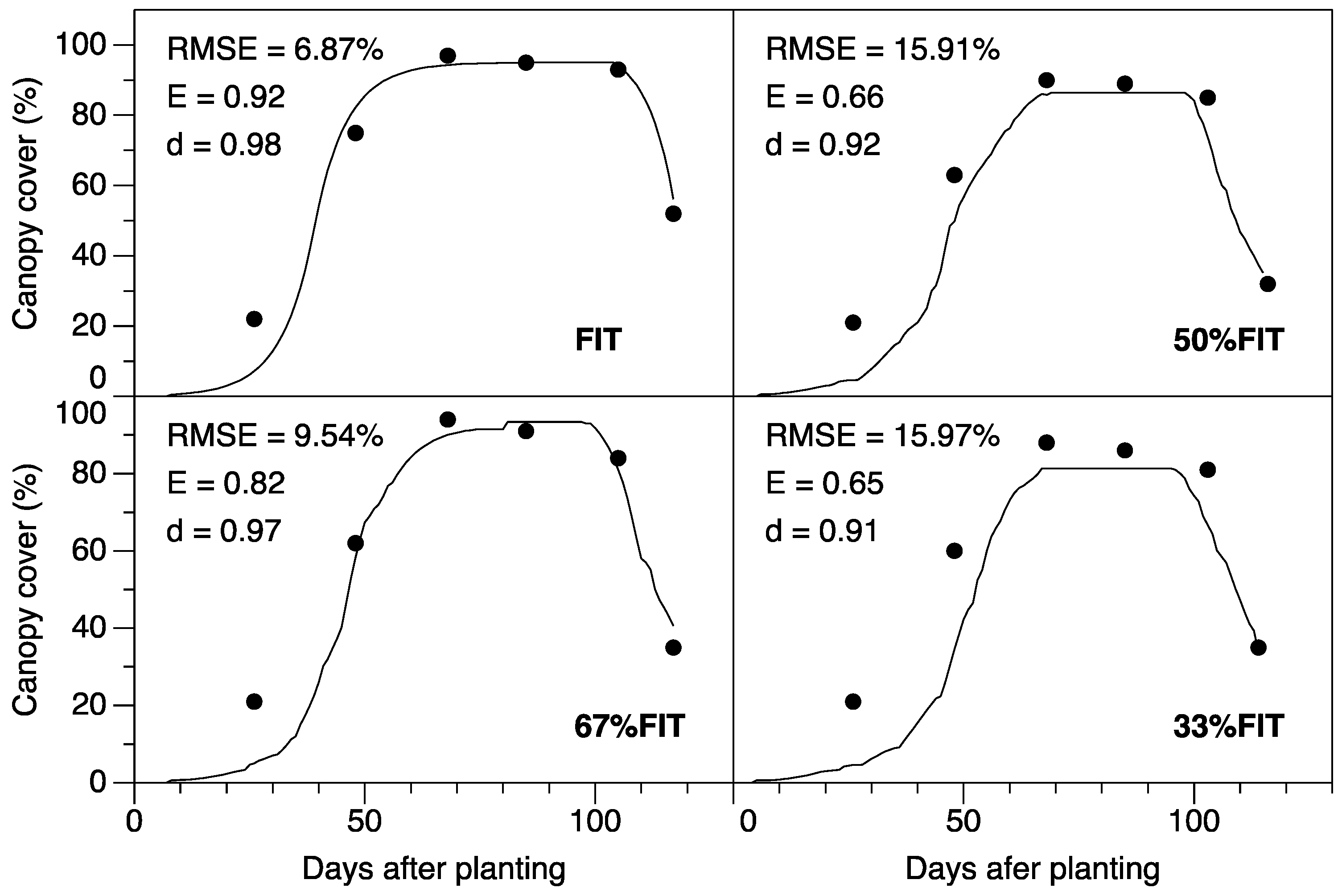However, in the severely stressed treatment (33% FIT) there was some mismatch between the model prediction and the observed values of daily B and CC, perhaps indicating that a change of these values, specifically stress threshold values, would improve the model simulation. Since the aim of the model calibration was to test for values that can work adequately under all conditions, the proposed values were maintained for use in predicting crop development and productivity as they worked well in non-stressed and moderately stressed conditions. Statistical indicators of RMSE, E, and d observed during the calibration process confirm this (Table 4). During the validation exercise it was observed that the performance of the AquaCrop depends on the water stress level experienced by the plants during the crop cycle and the output variable.

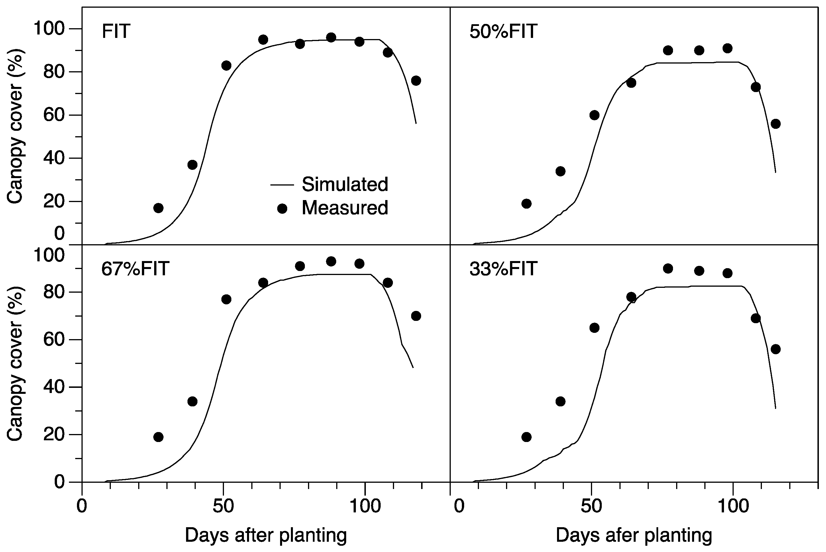
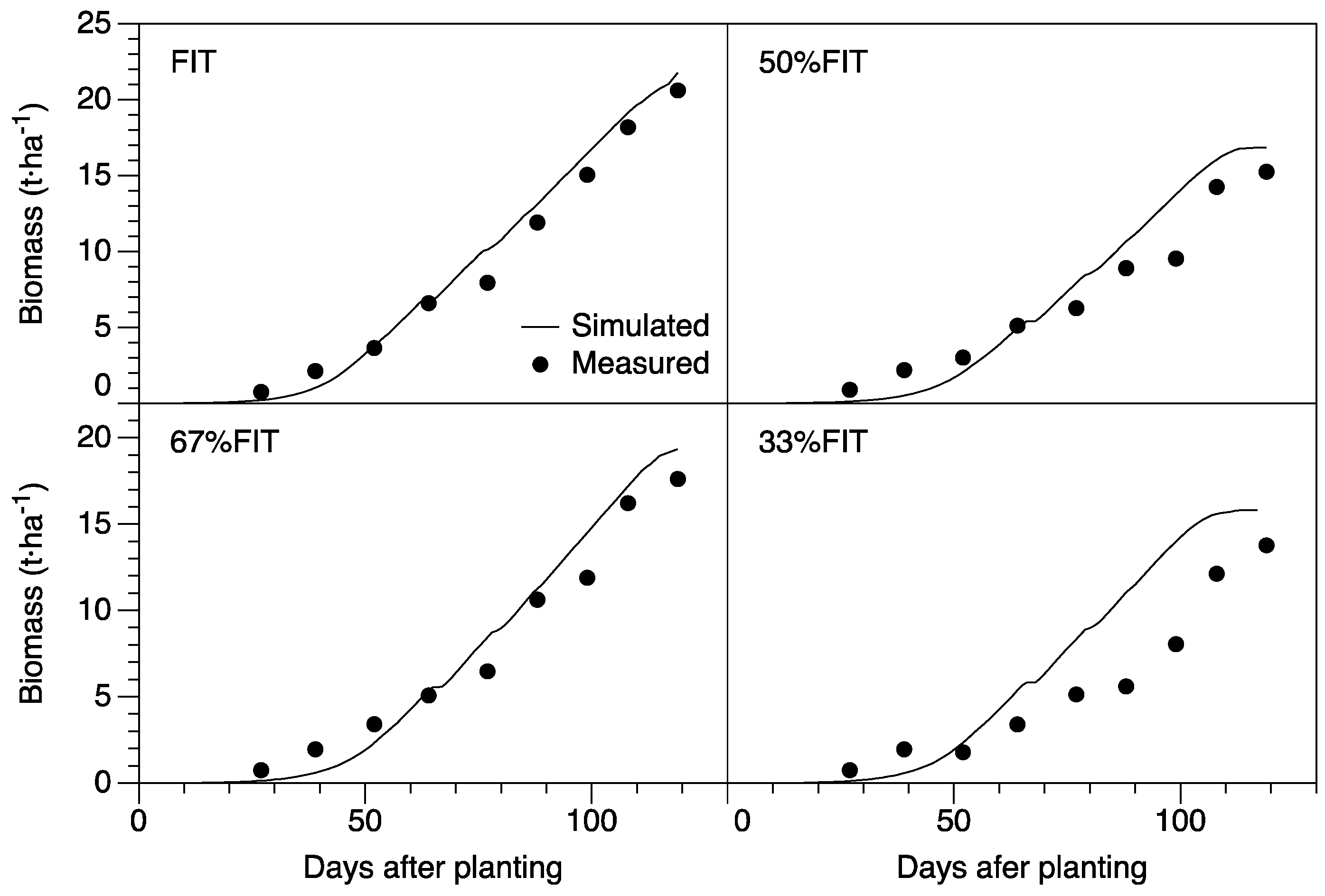
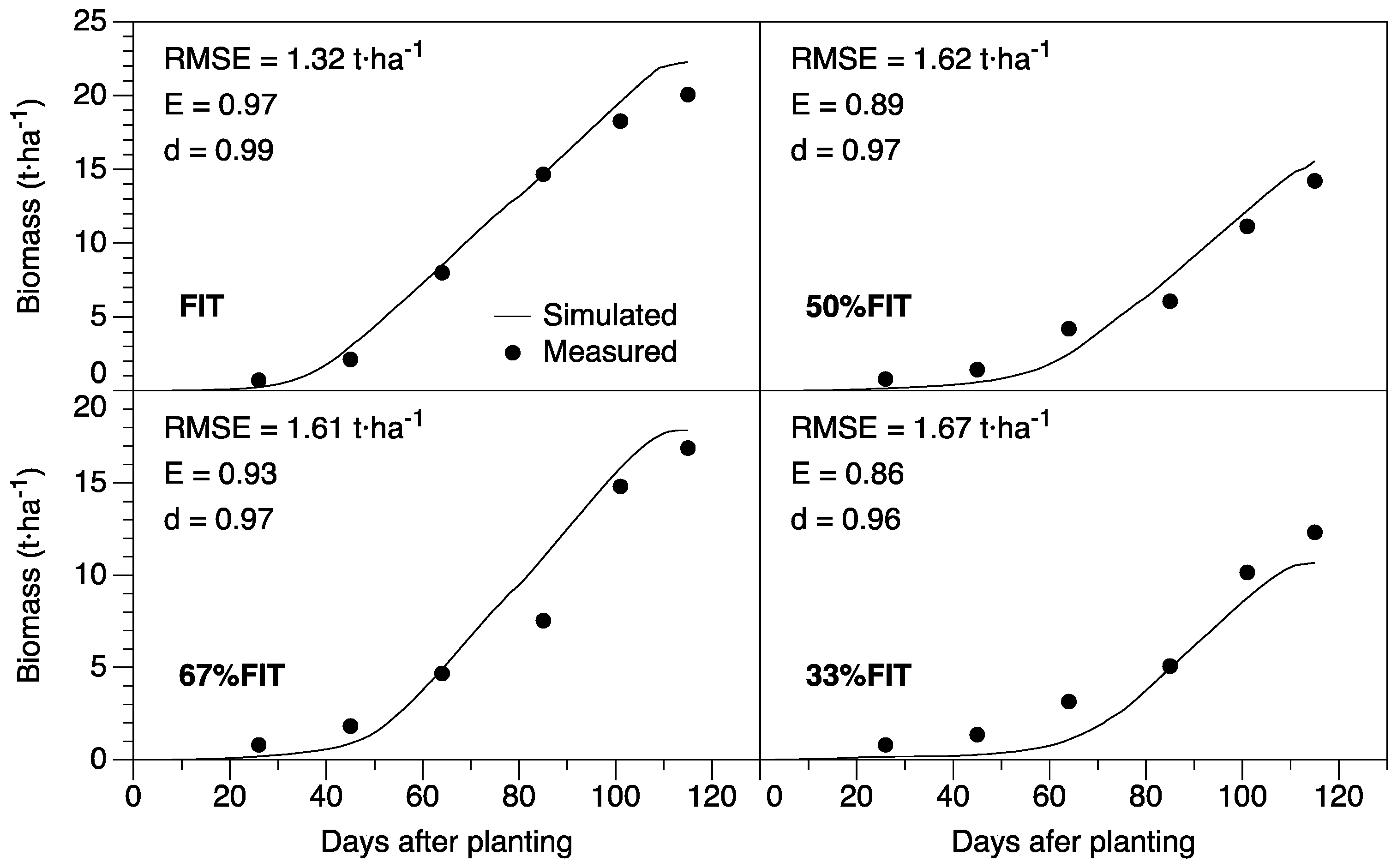
During the validation test, the seasonal evolution of CC was underestimated while the biomass was generally overestimated, except for the severely stressed treatment (33% FIT), where it was underestimated. Furthermore, the deviation between observed and simulated daily CC and biomass was more pronounced under water deficit conditions, becoming more intense as stress levels increased. The larger deviation between observed and simulated CC under water deficit and stress environments has also been reported for other crops like potatoes [15]. The general tendency of AquaCrop simulation model to overestimate maize biomass under water deficit conditions has been reported by Heng et al. [8], who contribute the deviation to vegetative stress and suggest that this can be attributed to the actual stomatal conductance being less than that simulated. Under the more severely stressed treatment of 33% FIT (Figure 6), the model underestimated the biomass through the whole season, which suggests that the model was not able to simulate the temporary relief from soil moisture stress due to irrigation application, unlike the other deficit treatments. For the other water deficit treatments of 67% FIT and 50% FIT, there was an initial underestimation of biomass up to about 60 DAP before overestimation. Observations made regarding a general whole-season underestimation of biomass for the more severely stressed treatment (33% FIT) was analogous to that reported by Katerji et al. [13] for maize and by Jin et al. [29] for winter wheat.

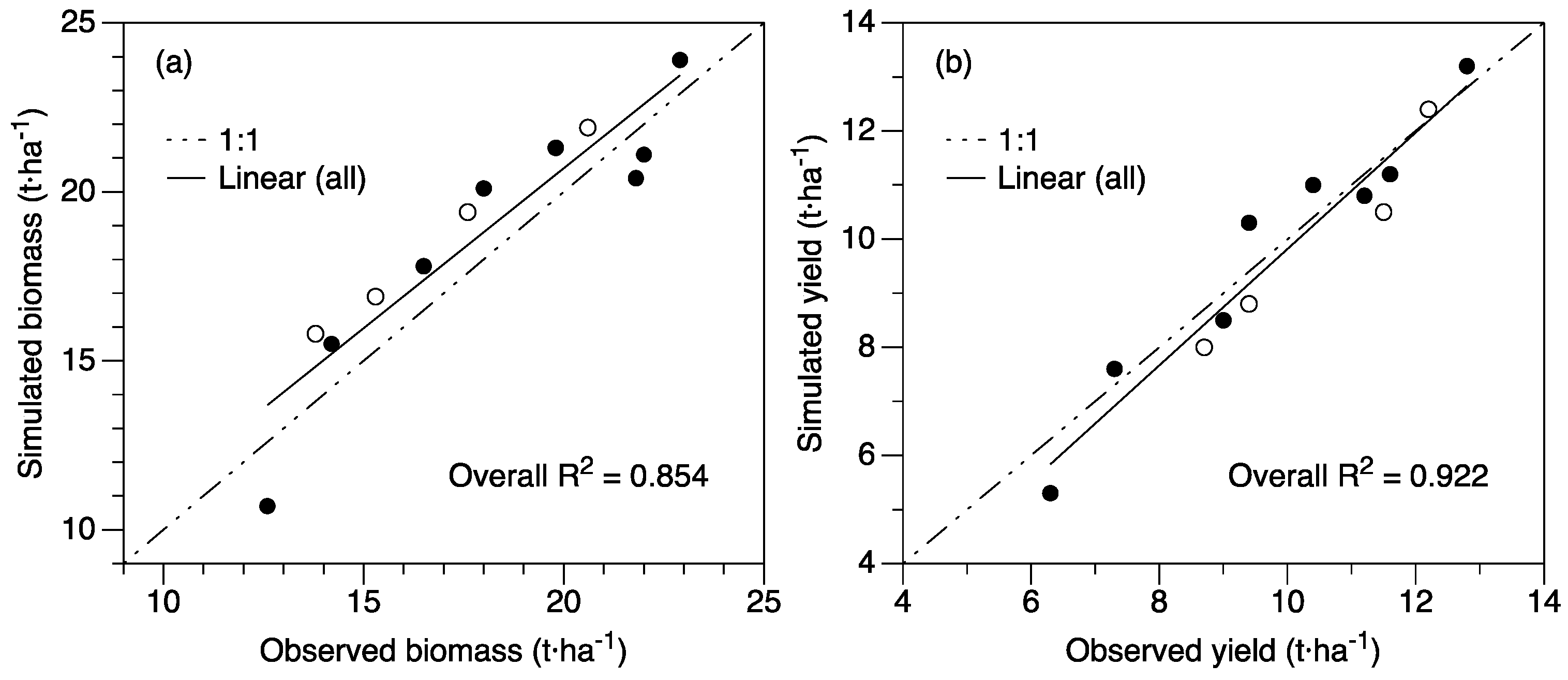
Simulated grain yields from Experiment 1 and 2 used in the validation exercise reduced on average by 19% for 67% FIT, 25% for 50% FIT, and 37% for 33% FIT with respect to the yield simulated under full irrigation. In comparison, measured yield reduction from the FIT was 11%, 21%, and 33% for 67% FIT, 50% FIT, and 33% FIT, respectively. The range of yield reduction for both measured and simulated data is similar to those reported by Katerji et al. [13] and García-Vila and Fereres [30]. These results imply that AquaCrop adequately predicts grain yield under varying environmental conditions, although the accuracy of the model declines in severely stressed conditions, confirming conclusions drawn from the two previously mentioned research. Furthermore, Katerji et al. 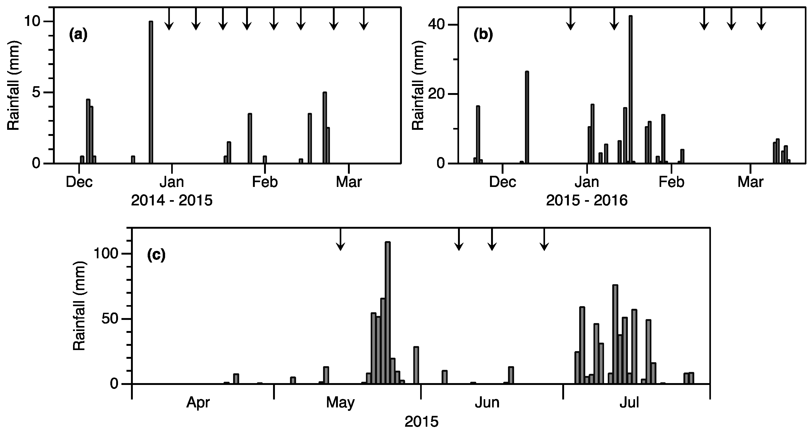[13] observed that in cases of severe moisture stress (based on a pre-dawn leaf water potential of −1.2 MPa), AquaCrop is unable to predict corn grain yield. Higher final biomass and grain yield were observed for maize sown in April (Experiment 2, Table 2). Two factors can account for this. First, for this season the soil moisture environment was better, reducing the length of the soil drought cycle on account of the rainfall. Rainfall would have had a significant impact on the experiment, as seen seeb by the four irrigation management applications, compared to the other seasons where irrigation application would have been the driving force behind the soil moisture environment. Secondly, during this cropping season the higher growing degree days would have promoted canopy growth and biomass accumulation, specifically during early developmental stages. According to Farahani et al. [3] and Jin et al. [29], the development of CC affects the rate of transpiration and consequently biomass and grain accumulation. Further studies manipulating the planting dates during the two distinct cropping seasons would be valuable.

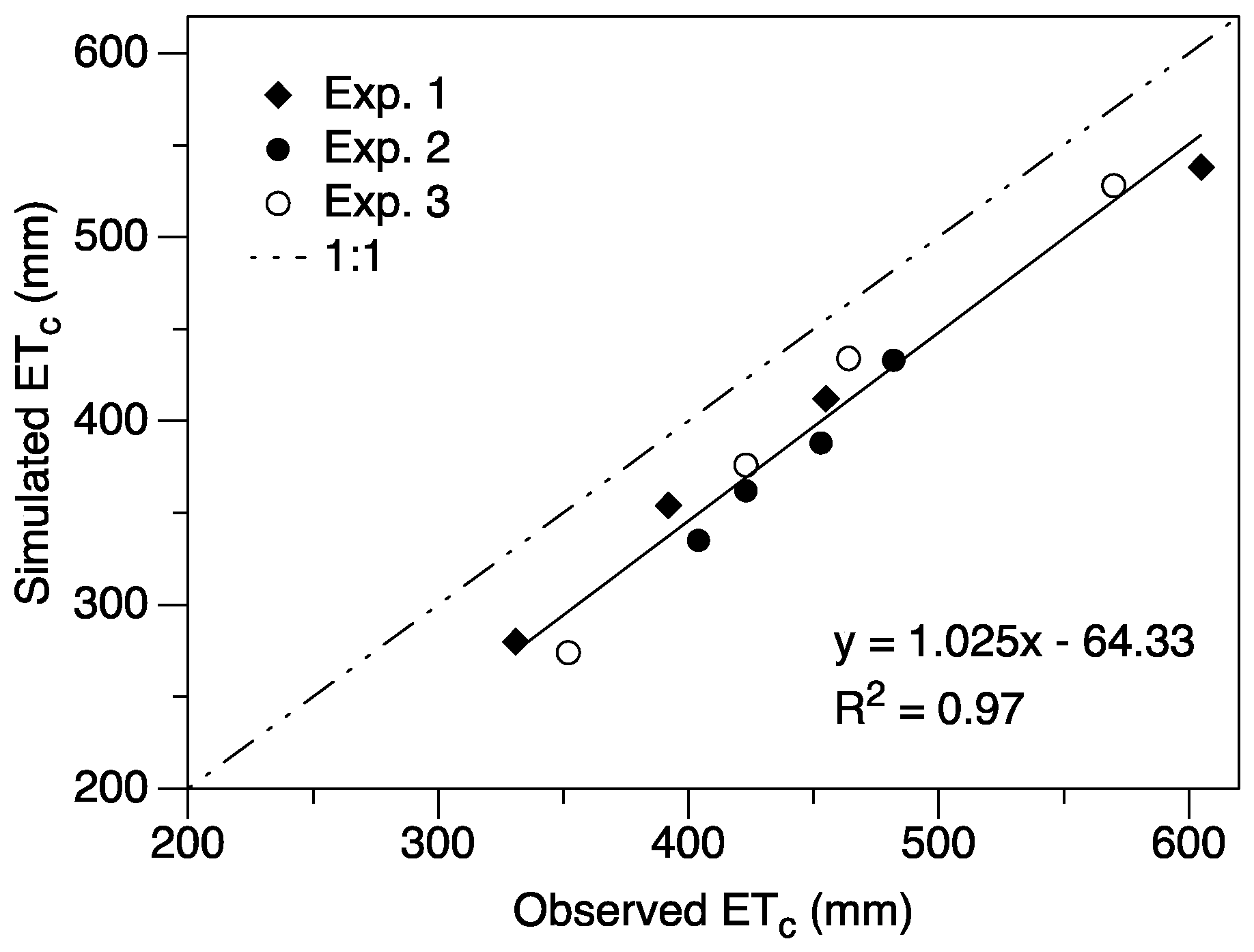
AquaCrop model was also tested for its ability to simulate seasonal ET_c and the WUE under different irrigation scenarios. Similar to the observations of Katerji et al. [13], AquaCrop systematically underestimated the seasonal ET and the deviations generally increased as stress levels intensified (Table 6). The range in reduction of 6.47% to 22.16% between simulated ET_c compared to observed values is higher than that reported by Heng et al. [8] during the validation of AquaCrop for maize, but less than the range of 5% to 37% for maize grown in varying levels of soil moisture stress observed by Katerji et al. [13]. In addition, the range calculated is similar for other crops grown in water deficit conditions like cotton [3] and tomato [31]. Large discrepancies between most values (8 out of 12 cases >10% deviation) can perhaps be attributed to the excessive drainage simulated by the model that was not observed in field measurements. Spatial variability of the soil could contribute to the discrepancy between observed and simulated results. Assumptions of uniform distribution of water in model simulations will inevitably lead to considerable differences in results of soil moisture content. In evaluating AquaCrop’s ability to simulate soil water content for pearl millet under irrigation and rainfed conditions, Bello and Walker [32] concluded that the model performance is moderate but needs considerable improvement. Further, simulated ET in AquaCrop is computed from the combination of soil evaporation and crop transpiration, which provokes some debate about the reliability. Katerji et al. [13] noted that while the measured ET values mainly reflect transpiration losses, simulated ET corresponds uniquely to soil evaporation, resulting in AquaCrop typically simulating low values of daily ET and overestimating the drought effect on this variable. Likewise, Farahani et al. [3] report that model estimation of soil evaporation is questionable because of the narrow range of soil evaporation observed across irrigation regimes, with large differences in application amount. Altering the conservative parameters used to directly simulate soil evaporation and crop transpiration like water extraction pattern, crop transpiration coefficient, and decline of crop coefficient was observed to have only a small change (low sensitivity level) on the simulated transpiration values. Thus, in most cases the defaulted values were maintained (Table 3). A low sensitivity level parameter indicates that the model response to change in input is generally less than 2% [7,24]. Geerts et al. [7] and Salemi et al. [24] reported similar observations for some of the abovementioned parameters.

Owing to some significant mismatch between simulated and observed ET_c values, the deviation between actual and simulated WUE of grain yield was large for most treatments (Table 6). However, the simulated values of WUE were similar to values reported in other studies for maize in varying soil moisture environments [8]. The large deviation of AquaCrop simulated WUE from field-estimated values has also been reported in other studies [4]. These authors report a deviation of up to 27% and 44% for sunflower grown under deficit irrigated and rainfed conditions, respectively, and a relatively low R² value (0.43) for the regression analysis of simulated WUE versus measured WUE. The large deviations observed in the study imply that there is considerable room for improvement in the model estimation of WUE, which relies heavily on predictions of crop ET. Evett and Tolk [28] suggest that AquaCrop only reliably simulates WUE under well-watered conditions but tended to misestimate WUE under conditions of water stress. Katerji et al. [13] further emphasize that AquaCrop’s performance in predicting WUE is especially unsatisfactory in cases of severe moisture stress.

The preceding discussion presented the response and resulting effectiveness of AquaCrop simulation model to different soil moisture environments. However, comparing the results between the two distinct cropping seasons used in the validation process (Experiments 1 and 2) presents another outlook to explore the efficacy of AquaCrop simulation model. Experiment 1 was subject to lower temperatures and small amounts of rainfall. In stark contrast, Experiment 2 was conducted in environments of higher temperatures, which are much more conducive for maize production, and extremely large amounts of rainfall. Evidently (Table 5), this resulted in productivity in terms of the biomass accumulation and yield procured being higher for Experiment 2. AquaCrop simulated these agronomic parameters adequately for both seasons, and in fact the relative difference between simulated and measured values was lower for Experiment 2 (Table 5). This suggests that the model, once properly calibrated, can be reliably used to make predictions of these variables in environments subject to extreme weather variability, and the calibrated model works reasonably well between distinct climate seasons. Furthermore, using the results from this field experiment allows for a more diverse dataset in the validation process. However, the extreme environments highlighted some limitations of the model, particularly its inability to predict ET_c and consequently crop WUE. For Experiment 2, the relative error (%) between the simulated and measured values for both ET_c and WUE was generally higher than in Experiment 1 (Table 6). This implies that the model reliability for these water variables decreases when challenged by extreme weather variations such as intense rainfall events and therefore reveals room for improving the model.

5. Conclusions

The AquaCrop model was tested and validated for its ability to simulate four crop parameters (green canopy cover (CC), biomass accumulation, and final biomass and grain yield at harvest) and two water variables (crop evapotranspiration (ET_c) and water use efficiency (WUE)) for full and deficit-irrigated maize in a tropical environment. Statistical indices of root mean square error, model efficiency, and index of agreement indicate that AquaCrop was able to simulate seasonal evolution of CC and biomass with a high degree of accuracy; however, model performance lessens as plant water stress intensifies. The high correlation of determination (R²) obtained in a 1:1 analysis indicates that the AquaCrop model adequately predicts final biomass and grain yield under different irrigation management strategies. An overall R² value of 0.85 and 0.92 was obtained for biomass and yield, respectively, using both calibration and validation datasets. The model was also able to simulate the seasonal ET_c and WUE to an appreciable degree, but model performance becomes unsatisfactory in severely stressed environments. Reduced model performance of ET_c and WUE, indicated by high deviation (%) estimates, can perhaps be attributed to the use of a single set of soil characteristics in the model calibration that does not reflect the spatial variability of the soil in the field. The results of this study suggest that the AquaCrop model could be used to predict biomass and yield with a high degree of reliability under various planting dates and irrigation management strategies. Thus, the model is a valuable tool to aid in decision-making for effective irrigation management strategies, but its predictive performance reduces in severely stressed soil moisture environments.

References

1. Toumi, J.; Er-Raki, S.; Ezzahar, J.; Khabba, S.; Jarlan, L.; Chehbouni, A. Performance assessment of AquaCrop model for estimating evapotranspiration, soil water content and grain yield of winter wheat in Tensift Al Haouz (Morocco): Application to irrigation management. Agric. Water Manag. 2016, 163, 219–235. [Google Scholar] [CrossRef]
2. Zhang, X.; Chen, S.; Liu, M.; Pei, D.; Sun, H. Improved water use efficiency associated with cultivars and agronomic management in the North China plain. Agron. J. 2005, 97, 783–790. [Google Scholar] [CrossRef]
3. Farahani, H.J.; Izzi, G.; Oweis, T.Y. Parameterization and evaluation of the AquaCrop model for full and deficit irrigated cotton. Agron. J. 2009, 101, 469–476. [Google Scholar] [CrossRef]
4. Todorovic, M.; Albrizio, R.; Zivotic, L.; Abi Saab, M.-T.; Stöckle, C.; Steduto, P. Assessment of AquaArop, CropSyst, and WOFOST models in the simulation of sunflower growth under different water regimes. Agron. J. 2009, 101, 509–521. [Google Scholar] [CrossRef]
5. Karunaratne, A.S.; Azam-Ali, S.N.; Izzi, G.; Steduto, P. Calibration and validation of FAO-AquaCrop model for irrigated and water deficient Bambara Groundnut. Exp. Agric. 2011, 47, 509–527. [Google Scholar] [CrossRef]
6. Rezaverdinejad, V.; Khorsand, A.; Shahidi, A. Evaluation and comparison of AquaCrop and FAO models for yield prediction of winter wheat under environmental stresses. J. Biodivers. Environ. Sci. 2014, 4, 438–449. [Google Scholar]
7. Geerts, S.; Raes, D.; Garcia, M.; Miranda, R.; Cusicanqui, J.A.; Taboada, C.; Mendoza, J.; Huanca, R.; Mamani, A.; Condori, O.; et al. Simulating yield response of quinoa to water availability with AquaCrop. Agron. J. 2009, 101, 499–508. [Google Scholar] [CrossRef]
8. Heng, L.K.; Hsiao, T.; Evett, S.; Howell, T.; Steduto, P. Validating the FAO AquaCrop model for irrigated and water deficient field maize. Agron. J. 2009, 101, 488–498. [Google Scholar] [CrossRef]
9. Steduto, P.; Hsiao, T.C.; Raes, D.; Fereres, E. AquaCrop-The FAO crop model to simulate yield response to water: I. concepts and underlying principles. Agron. J. 2009, 101, 426–437. [Google Scholar] [CrossRef]
10. Raes, D.; Steduto, P.; Hsiao, T.C.; Fereres, E. AquaCrop-The FAO crop model to simulate yield response to water: II. Main algorithms and software description. Agron. J. 2009, 101, 438–447. [Google Scholar] [CrossRef]
11. Raes, D.; Steduto, P.; Hsiao, T.C.; Fereres, E. AquaCrop Reference Manual; Version 4; FAO—Land and Water Division: Rome, Italy, 2012. [Google Scholar]
12. Hsiao, T.C.; Heng, L.; Steduto, P.; Rojas-Lara, B.; Raes, D.; Fereres, E. AquaCrop-The FAO crop model to simulate yield response to water: III. Parameterization and testing for maize. Agron. J. 2009, 101, 448–459. [Google Scholar] [CrossRef]
13. Katerji, N.; Campi, P.; Mastrorilli, M. Productivity, evapotranspiration, and water use efficiency of corn and tomato crops simulated by AquaCrop under contrasting water stress conditions in the Mediterranean region. Agric. Water Manag. 2013, 130, 14–26. [Google Scholar] [CrossRef]
14. García-Vila, M.; Fereres, E.; Mateos, L.; Orgaz, F.; Steduto, P. Deficit irrigation optimization of cotton with AquaCrop. Agron. J. 2009, 101, 477–487. [Google Scholar] [CrossRef]
15. De Casa, A.; Ovando, G.; Bressanini, L.; Martínez, J. Aquacrop model calibration in potato and its use to estimate yield variability under field conditions. Atmos. Clim. Sci. 2013, 3, 397–407. [Google Scholar]
16. Perng, C.M. Taiwan Grain and Feed Annual Wheat, Corn and Milled Rice Situation and Outlook; USDA Foreign Agriculture Service: Taipei, Taiwan, 2013.
17. COA, E.-Y. The Development of High Quality Corn Industry in Taiwan. Available online: http://flora.coa.gov.tw/view_eng.php?id=131 (accessed on 15 May 2015).
18. Allen, R.G.; Pereira, L.S.; Raes, D.; Smith, M. Crop Evapotranspiration: Guidelines for Computing Crop Requirements; Food and Agriculture Organization of the United Nations: Rome, Italy, 1998. [Google Scholar]
19. Panda, R.K.; Behera, S.K.; Kashyap, P.S. Effective management of irrigation water for maize under stressed conditions. Agric. Water Manag. 2004, 66, 181–203. [Google Scholar] [CrossRef]
20. Djaman, K.; Irmak, S.; Rathje, W.R.; Martin, D.L.; Eisenhauer, D.E. Maize evapotranspiration, yield production functions, biomass, grain yield, harvest index, and yield response factors under full and limited irrigation. Am. Soc. Agric. Biol. Eng. 2013, 56, 273–293. [Google Scholar]
21. Igbadun, H.E.; Salim, B.A.; Tarimo, A.K.P.R.; Mahoo, H.F. Effects of deficit irrigation scheduling on yields and soil water balance of irrigated maize. Irrig. Sci. 2008, 27, 11–23. [Google Scholar] [CrossRef]
22. Yi, L.; Shenjiao, Y.; Shiqing, L.; Xinping, C.; Fang, C. Growth and development of maize (Zea mays L.) in response to different field water management practices: Resource capture and use efficiency. Agric. For. Meteorol. 2010, 150, 606–613. [Google Scholar] [CrossRef]
23. Doorenbos, J.; Kassam, A.H. Yield Response to Water; Food and Agriculture Organization: Rome, Italy, 1979. [Google Scholar]
24. Salemi, H.; Soom, M.A.M.; Lee, T.S.; Mousavi, S.F.; Ganji, A.; KamilYusoff, M. Application of AquaCrop model in deficit irrigation management of Winter wheat in arid region. Afr. J. Agric. Res. 2011, 6, 2204–2215. [Google Scholar]
25. Nash, J.E.; Sutcliffe, J. V River flow forecasting through conceptual models: I. A discussion of principles. J. Hydrol. 1970, 10, 282–290. [Google Scholar] [CrossRef]
26. Willmott, C.J. Some comments on the evaluation of model performance. Bull. Am. Meteorol. Soc. 1982, 63, 1309–1313. [Google Scholar] [CrossRef]
27. Zeleke, K.T.; Luckett, D.; Cowley, R. Calibration and testing of the FAO AquaCrop model for canola. Agron. J. 2011, 103, 1610–1618. [Google Scholar] [CrossRef]
28. Evett, S.R.; Tolk, J.A. Introduction: Can water use efficiency be modeled well enough to impact crop management? Agron. J. 2009, 101, 423–425. [Google Scholar] [CrossRef]
29. Jin, X.-L.; Feng, H.-K.; Zhu, X.-K.; Li, Z.-H.; Song, S.-N.; Song, X.-Y.; Yang, G.; Xu, X.-G.; Guo, W.-S. Assessment of the AquaCrop model for use in simulation of irrigated winter wheat canopy cover, biomass, and grain yield in the North China plain. PLoS ONE 2014, 9, e86938. [Google Scholar] [CrossRef] [PubMed]
30. García-Vila, M.; Fereres, E. Combining the simulation crop model AquaCrop with an economic model for the optimization of irrigation management at farm level. Eur. J. Agron. 2012, 36, 21–31. [Google Scholar] [CrossRef]
31. Darko, R.O.; Shouqi, Y.; Haofang, Y.; Junping, L.; Abbey, A. Calibration and validation of Aquacrop for full and deficit irrigation of tomato. Int. J. Agric. Biol. Eng. 2016, 9, 104–110. [Google Scholar]
32. Bello, Z.A.; Walker, S. Calibration and validation of AquaCrop for pearl millet (Pennisetum glaucum). Crop Pasture Sci. 2016, 67, 948–960. [Google Scholar] [CrossRef]
Figure 1. Daily rainfall at the experimental site over the three cropping seasons: (a) November 2014 to March 2015; (b) November 2015 to March 2016; (c) April to July 2015. Arrows at the top indicate the time of irrigation application (from V6 growth stage) for all treatments.
Water 08 00557 g001
Figure 2. Simulated and measured canopy cover for the different irrigation treatments used for AquaCrop calibration.
Water 08 00557 g002
Figure 3. Seasonal evolution of measured and simulated aboveground biomass for the different irrigation treatments used for AquaCrop calibration.
Water 08 00557 g003
Figure 4. Relation between measured and simulated values for (a) biomass and (b) grain yield for the calibration dataset (open circle) and validation dataset (filled circle).
Water 08 00557 g004
Figure 5. Simulated and measured canopy cover for the four irrigation treatments in Experiment 1 used in model validation.
Water 08 00557 g005
Figure 6. Seasonal progression of simulated and observed aboveground biomass used in model validation.
Water 08 00557 g006
Figure 7. Comparison between measured and simulated seasonal evapotranspiration (ETc) for all treatments over the three experimental (Exp.) periods.
Water 08 00557 g007