Paleohydraulic Reconstruction of Modern Large Floods at Subcritical Speed in a Confined Valley: Proof of Concept

Abstract

The present study aims to show the accuracy of paleoflood reconstruction techniques based on two-dimensional (2D) hydraulic modelling of a large flood. Using this reconstruction technique, we determined trends in flood stages over time in a regulated river. A stretch of the Guadalquivir River (Southern Spain) was selected as the study site. High-resolution orthophotos and LiDAR (Light Detection and Ranging) elevations were acquired just after modern floods. They were used for the identification and location of stage indicators. In addition, water gradients were estimated from gauging records, documentary information and paleostage indicators (PSIs) in two situations: (i) pre-vegetation encroachment; and (ii) post-vegetation encroachment due to upstream impoundment. Standard two-dimensional, flow depth-averaged equations over fixed beds were used in the hydraulic modelling. In a first stage, long records of instrumental data at gauging stations and documentary evidence of flood levels served to calibrate the input parameters of the hydraulic model. In a second stage, paleoflood signatures within sedimentary and botanical sequences served to verify the flood stages in the numerical simulations not only at the river reach where instrumental data exist but also in the downstream river reach. Interestingly, the rating curve obtained from the combined use of documentary information and imagery was nearly as accurate as gauging measurements. The thoughtful comparison of 2D modelled hydraulic variables against inferred values from PSIs and instrumental data supports the paleoflood reconstruction method over fixed beds. Vegetation encroachment provoked 10% deeper floods at the water discharge of 2000 m³$·$s⁻¹, which implied an increase of Manning’s roughness coefficient from 0.04 to 0.055 s$·$m^−1/3 in less than 15 years.

1. Introduction

Indirect estimation techniques of peak water discharges such as slope-conveyance, slope-area method, one- and two-dimensional hydraulic modelling are frequently used in paleoflood hydrology [1], reconstructions of glacial-lake outburst floods [2,3,4], mega-floods [5,6,7,8] and extreme floods with stream gauges damaged during the event [9]. Large flood at subcritical speed could develop in a bedrock stream down a low slope, a preferred configuration to apply the paleoflood reconstruction method [10]. Paleoflood hydrology also addresses supercritical flow regimes developing, for instance, during extreme flash floods over steep bottom slopes in ungauged catchments and mountainous watersheds [11,12]. However, large floods typically prevent the verification of the inferred peak water discharge by comparison with in situ measurements [1,10].

Paleohydrology was originally based on non-systematic data as sedimentological and botanical PSIs [1,13]. The reliability of PSIs for paleoflood studies is well established [14,15]. High-water marks (HWMs) [16] are the most useful source of information on establishing grade lines [14]. Non-systematic data can be combined with systematic data [9]. In so doing, temporal and spatial patterns of extreme river events can be better predicted [17]. This method is a significant tool for flood risk analysis and to gain insight into the long-term flood regime dynamics [18]. Indeed, the utility of documentary evidence to lengthen flood records of rare and extreme events has recently been pointed out [19,20,21]. In the case in which the discharge-stage curve exists from direct field measurements as a gauging station, there is no need to retrodict the peak water discharge using paleohydrology [22]. Yet, the comparison of hydrological data against modelled hydraulic variables serves to evaluate the accuracy of the paleohydraulic reconstruction. Note that the comparison is not part of the standard reconstruction, but that it is an original method of verification proposed in this paper.

Two-dimensional hydraulic modelling has become a standard in paleohydrology [2,3,7,23,24,25] similar to slope-conveyance, slope-area methods and step-backwater analysis [11,26,27]—perhaps due to recent advances in computational power, the availability of Digital Elevation Models (DEM) and open-source 2D codes, e.g., DassFlow-Shallow [28,29]. Guidelines in the development and application of computational methods to environmental fluid mechanics, including quantification of uncertainty and model testing, can be found in [30]. Key inputs for the schematisation of 2D models that use the Saint-Venant equations are the hydraulic roughness of the surface, the 2D channel geometry, and the boundary conditions (BCs). The first is determined using Manning’s parameter [11] or, alternatively, by means of Darcy-Weisbach friction factor [3,31]; the second is based on high-resolution digital terrain models or surveys of channel depth [32]. Lastly, two types of BCs are required when solving numerically the shallow-water equations [33]: physically based (e.g., inlet water discharge and outlet flow depth) and numerical BCs (e.g., characteristic variable extrapolation). Taking into account that BCs mimic the behaviour of the flow variables on the border of the inner computational grid and the misrepresented outer domain [30], sensitivity to boundary conditions needs to be addressed by considering different extensions of the simulated channel and accurate modelling of the flow outside of the area of paleohydrological interest.

The main aim of this article is to evaluate the accuracy of standard paleohydraulic reconstruction methods based on the comparison of modelled hydraulic variables from two-dimensional shallow water equations over fixed beds and a rich set of hydrological data. Previously undocumented floods at subcritical speeds in the Guadalquivir River were considered in this study. The co-existence of hydrological records from multiple sources allowed splitting the full data set into two subgroups, which were used in the following steps of the study: (i) gauging records served to calibrate the input parameters of the hydraulic model; (ii) additional hydrological information (i.e., PSIs, historical imagery of floods and series of orthophotos) corresponding to recent floods was employed to verify the accuracy of the 2D paleohydraulic reconstruction. Furthermore, understanding of trends in flood stages over time was finally achieved thanks to the combined interpretation of hydrological evidence and modelled hydraulic variables.

The paper is organised as follows: Materials and Methods (i.e., the description of the study site, the sources of hydrological data and an overview of the hydraulic modelling technique) are presented in Section 2. Experimental and numerical results are described in Section 3. Conclusions are finally presented in Section 4.

2. Materials and Methods

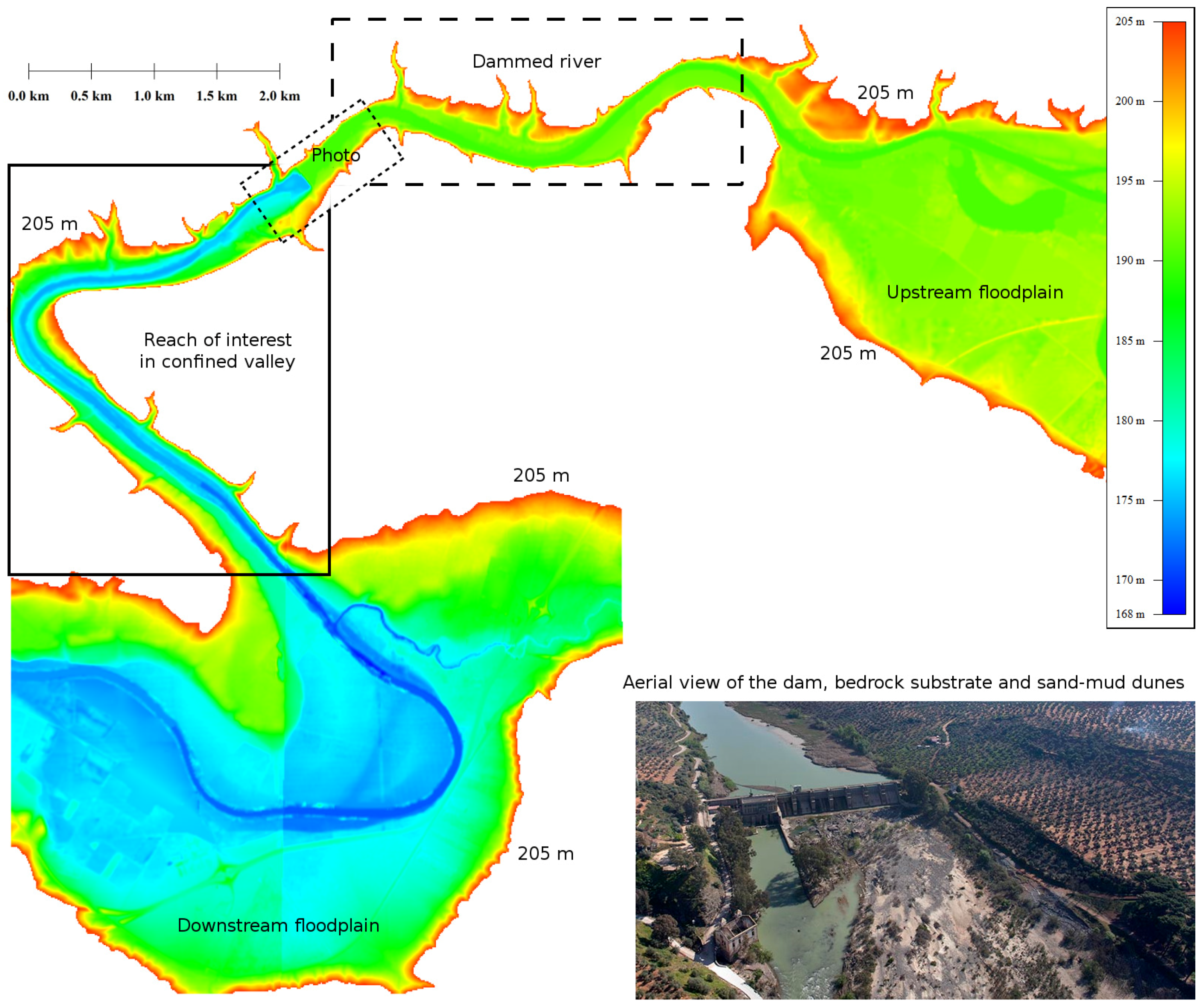
2.1. Study Area

The field area is situated along a stretch of the Guadalquivir Valley on the border of the provinces of Jaén and Córdoba, Southern Spain (Figure 1). The fluvial regime is typically Mediterranean, showing a summer drought period with minimum water levels and highest values in winter and spring. Different climate influences of the Mediterranean Sea and the Atlantic Ocean, the complex topography and the size of the drainage area (19,546 km²) favour the occurrence of heavy precipitation events and floods [34]. Indeed, flooding is the most damaging type of natural disaster in this area [35] with economic losses per province ranging between 200 and $1200\times {10}^6$ € [36]. In this study, previously undocumented extreme floods occurred since the early 20th century are analysed in a channel reach of the confined valley downstream of the Marmolejo dam (N ${38}^{\circ }$$3^{\prime }$${31}^{″}$ E $4^{\circ }$${11}^{\prime }$${13}^{″}$), see the sketch in Figure 1.

The inlet of the selected study reach is a bedrock channel of 750 m length and 190 m width with the exposed slate substrate where transport capacity exceeds sediment supply [37,38]. Characteristic flow depths during large floods are about 10 m for $Q=2000$ m³$·$s⁻¹ (Q denotes water discharge from now on). The full reach of interest is 6 km in length and exhibits a sharp bend of approximately 140 degrees and 400 m radius that joins two straight channels of 100–200 m bankfull width. It is interpreted as a transfer area between less stable floodplains at the up- and down-stream boundaries [39,40], recall Figure 1. The slope of the channel thalweg is very low (mean value of 0.076%) leading to subcritical flow regime and downstream hydraulic control at all water discharges, referred to as backwater effect [41], as it happens in large flood flow in narrow deep bedrock streams [10]. An additional constraint in the study site is the need to minimise the impact of natural or anthropogenic channel changes, river engineering works and land-use change. Hence the dammed upstream channel reach has only been used to establish well-controlled boundary conditions, being excluded in the paleoflood study.

Such simple hazardous site mimics a laboratory flume at a much larger real scale. It is well-gauged and favours the quantification of the influence of each input factor on the paleohydraulic reconstruction results. Furthermore, it satisfies Baker’s rules on paleohydrology [10]:

• The study site must be selected in order that the flood discharge increases result in large increases in the stage. Thus, the confined channel is more preferred than the floodplains. Indeed, an increase in the water discharge from 1400 to 3000 m³$·$s⁻¹ implies an increase in depth of 4 m in the main channel of the confined valley analysed herein (see Section 3).
• It is important to find key control reaches with stable cross-sections and well-preserved high-water indicators. Subsequently, a channel with exposed slate substrate and bedrock gorge was selected in this study, allowing the use of two-dimensional shallow water equations over fixed bed in the hydraulic reconstruction [3,8].

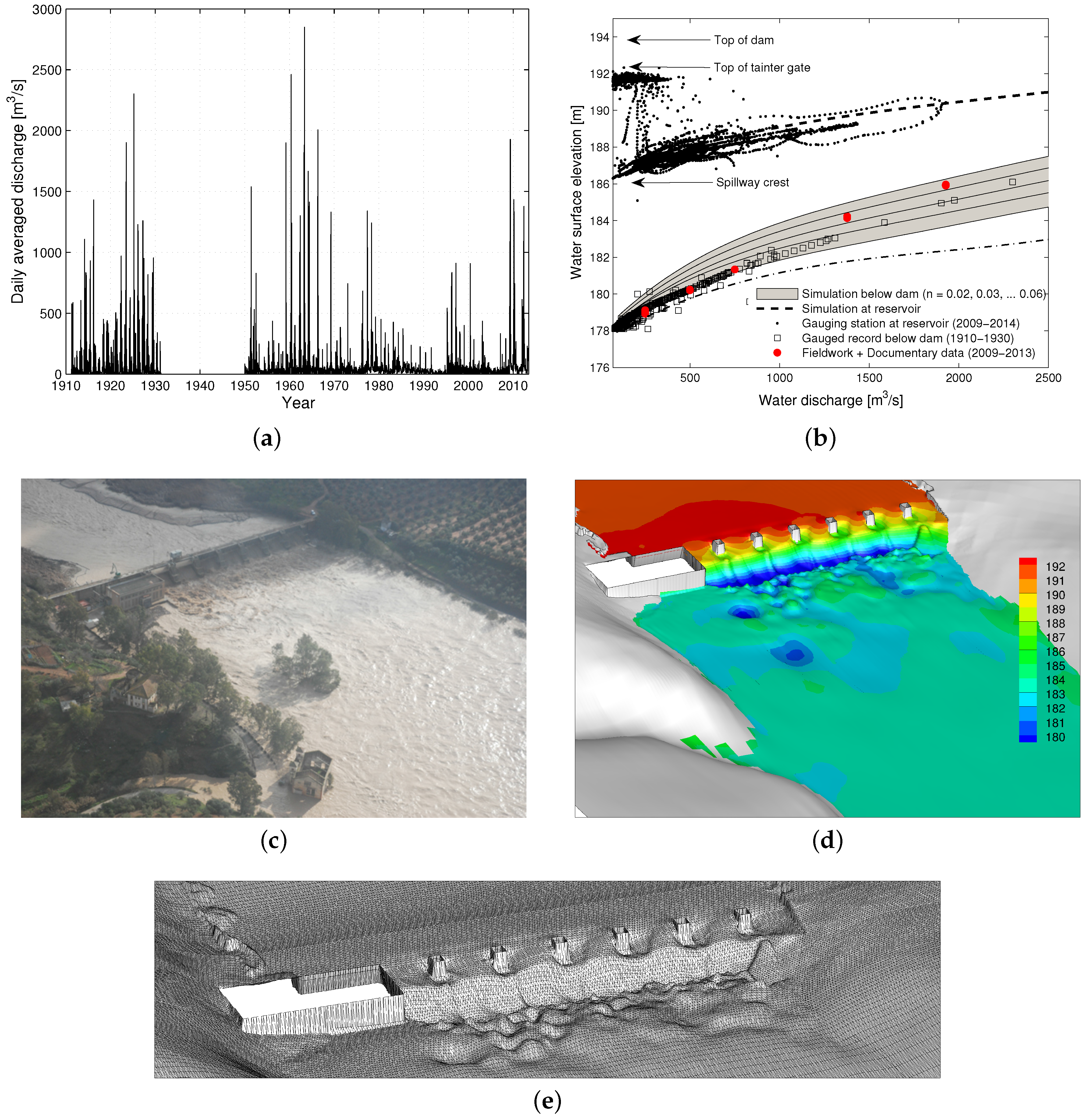
2.2. Gauging Records

Systematic recording of daily average water discharge began in 1911 with the publication of the annual review of gauge stations [42,43]. Since the year 1989, a national net for real-time hydrologic monitoring provides hourly average values [44].

Local records are available at three hydropower stations during different periods. Two of them are readily observed in the inset of Figure 1 as well as in Figure 2c. The oldest one supplied local demands of electricity between the years 1911 and 1926. Presently, it is submerged because the actual station was built few meters downstream. One can still observe the powerhouse that operated downstream of the actual dam between the years 1926 and 1962, see the old building at the bottom of Figure 2c. Gauging records could be merged into a single series because of the proximity of the three stations. Hence, systematic records of annual peak flows based on daily average water discharge were obtained since 1911. In addition to the water discharge records, the free-surface elevation was measured below the dam and at the reservoir during the periods 1911–1930 and 2009–2013, respectively. These data are shown in Figure 2 and further commented in Section 3.1.

2.3. Imagery and Documentary Evidence

Scarce, discontinuous documentary record without flood stage data in the Guadalquivir River starts during the Arabian period in Córdoba (711) and Sevilla (849) up to 1400 [45,46]. Nearly complete data series of the magnitude and frequency of documentary floods in these provinces were compiled by Borja Palomo [47] from 1400 to the late 19th century based on public and ecclesiastic archives. However, the first inundation in the province of Jaén was not recorded until 1618 in the city of Andújar and the total number of records in the province only amounts to the low value of 17 before 1900, which is much lower than the 183 floods reported in Córdoba and Sevilla [45].

In order to lengthen flood records of extreme events, imagery was collected from the following sources: in situ photographs (1906–2013), aerial photographs from helicopter surveys (2009–2013) and sequences of orthophotos (1945–2013). In situ photographs are available at two local stations with a sampling frequency of hours or days during modern floods (2009–2013). Older photographs are available as a documentary evidence. Aerial photographs were acquired from helicopter flights during the occurrence of peak water discharges in 2009–2013 floods. Orthophotos are periodically updated in southern Spain since 1998, with a frequency of 2 years, whilst the previous sampling frequency varies between 7 and 20 years. Thus, the combination of the three sources of information enriches the description of floods by increasing both the temporal sample rate and the spatial resolution.

On the one hand, in situ photographs were available at two stable cross sections—the dam (Figure 2) and an old bridge/Spa (Figure 3) located 775 m further downstream (see locations in Figure 4a). On the other hand, aerial photographs (e.g., Figure 2c) delimited the inundated area during modern floods from the dam to the river bend. Imagery was used to infer the water surface elevation for known water discharges as follows: firstly, fieldworks were conducted with the main aim of positioning the highest watermark from the photos by using a modern laser Leica DISTO^TM S910 (Swiss technology); next, rating curves were obtained below the dam and at the bridge/Spa by correlating the date and time of the photo with the inferred flood stage and the water discharge (known at the dam).

The third set of imagery is series of orthophotos [48]. Orthophotos cover the whole Guadalquivir basin. Also, orthophotos depict the evolution of the river through time since 1945, see Figure 4. The main channel and the floodplains have experienced minor changes due to soil management by farmers, the growth of riparian vegetation and sedimentation of slackwater deposits during large floods. The orthophoto of the year 2013 was particularly useful to locate the most elevated slackwater deposits along the riversides. It allowed the identification of PSI-HWMs and the delimitation of the inundated area after the most recent flood (April 2013). For instance, the solid lines in Figure 4a depict the area of such inundation based on fine sediment deposits, which extends nearly along the whole reach of interest. Other statistics as the channel width and the wetted area could be studied but they lie out of the scope of the paleoflood analysis. Unfortunately, such procedure could not be applied for older floods because the natural cover in the orthophotos prevents the identification of flood deposits.

2.4. Sedimentary Sequences and Botanical High Watermarks

Well-preserved PSIs were identified in post-event fieldworks between October 2015 and May 2016. A rich collection of subreach-scale morphologic units developed during 2009–2013 floods thanks to the large availability of fine sediments (mud, silt and clay) in the silted reservoir.

Sediments settled in the reservoir during high water stages just after the construction of the dam, mostly during the period 1963–2001. Figure 2c illustrates this point by showing the top level of sediments in the reservoir as elevated as the spillway crest and the water level in February 2010. This situation is not isolated as more severe states are found out in the three reservoirs located 67 km upstream (presently silted up to $98\%$), as reported by Bohorquez et al. [49]. Reservoirs do not have bottom withdrawal spillways, could not retain sediments during the 2010–2013 floods and, consequently, a large amount of sediments was supplied from Marmolejo dam. This favoured the developments of numerous slackwater deposits.

PSIs were located with GPS and laser Leica DISTO^TM S910, see some illustrative examples in Figure 5. Then, the highest elevation of the PSIs was positioned as a function of the streamwise distance to the dam (denoted by x). In a longitudinal downstream profile, the following sedimentary sequences were identified: erosional reach with exposed bedrock shales at the foot of the dam ($x\le 175$ m, see inset in Figure 1); imbrication of cobbles, pebbles and clasts pointing in the downstream direction few meters downstream ($175<x\le 325$ m, see Figure 5c); field of longitudinal sand bumps in mixed sand-mud ($325<x\le 425$ m, see again Figure 5c); laterally-attached sandy siltlines emplaced from suspension where flow boundaries (bridge peers, Spa building, bend and shoreline) produce markedly reduced local velocities relative to the mean channel velocity ($850<x\le 5000$ m, see e.g., solid line in Figure 4a); bar formation at natural channel bend ($2580<x\le 2630$ m, see Figure 5a); and, preservation of relatively fine-grained flood sediments deposited at tributary mouth slackwater site where the Guadalquivir flooding backflood the tributary up to a level equivalent to the mainstream flood stage ($x\approx 6000$ m).

Additionally, flood botanical records are abundant along the whole reach of study. Leaves debris occurs at the branches of riparian trees. Woody debris accumulates upstream of trunks and deposits at the bottom surface. Riparian trees also show scars on their trunks. The highest level marks are well elevated above the thalweg and serve to establish botanical HWMs.

2.5. Two-Dimensional Shallow Water Modelling, Computational Mesh and Boundary Conditions

This section shows how the computational mesh was constructed to avoid modelling errors associated with the uncertainty of physical/numerical boundary conditions needed by the two-dimensional Saint-Venant equations. As the numerical simulation technique has been detailed previously at length in Author’s previous works [3,12,49], I will not dwell on this issue. However, a summary explanation is needed.

Recirculation zones and complex non-uniform velocity fields may develop in the presence of hydraulic infrastructures, the sudden expansion/contraction of the channel, in natural river bends and floodplains. Such flow patterns are well resolved by the 2D Saint-Venant equations which also capture backwater effects, hydraulic jumps, the backflood of tributary and wet/dry fronts [50]. Hence the 2D unsteady shallow-water model implemented in the open-source code Dassflow-Shallow 2.0 was adopted in this study [29]. Simulated flooding areas, maps of water flow depth and two-dimensional velocity vectors were obtained by solving numerically the two-dimensional unsteady shallow water equations. The hyperbolic problem with source terms was solved using a second-order accurate HLLC approximate Riemann solver with MUSCL reconstruction, and an implicit-explicit Runge-Kutta (IMEX) time integration—denoted by IMEX-SSP(3,2,2)/MUSCL with MP limiter in Monnier et al. [29]. The time step in the numerical simulations was adjusted dynamically during the simulation process in order to satisfy the Courant-Friedrich-Lewy (CFL) stability condition [51].

To avoid the influence of the boundary conditions on the numerical results at locations of interest, the extent of the computational domain was chosen from the reservoir of the dam (inlet) to the floodplain (outlet) shown in Figure 1. Whereas the reach of interest for the paleohydraulic study lies at the foot of the dam up to the end of the confined valley, the real geometry of the dam and the reservoir have been taken into account in the geometrical modelling. Furthermore, the computational mesh extends far away from the outlet of the confined valley. In particular, the floodplain depicted in Figure 1 forms a part of the computational domain. In doing so, the outlet boundary conditions are applied far from the reach of interest and, consequently, numerical results in the confined valley are independent of the outlet conditions [30]. The computational mesh was created by patching the 5 m resolution DEM [52] in Figure 1 with the reservoir bathymetry (obtained from SONAR measurements) and the dam/spillways geometry (measured in situ with the Leica DISTO^TM S910). A computational mesh with a cell size thinner than 1 m was created near the spillways, see Figure 2). Far from the dam, the computational grid is coarser with characteristic edge lengths of 5 m in the channel and 10 m in the valley. The mesh of the reservoir, dam and spillway piers replicates reality. Note the similarity between the simulated geometry (Figure 2e) and the real one (Figure 2c).

A similar approach could be adopted in movable bed conditions by using the pre-flood DEM and replacing the Saint-Venant equations over fixed beds with a hydro-morphodynamic model [53,54]. The lack of hard information on how particle diffusivity, entrainment and deposition rates vary with flow conditions and sediment supply, see Bohorquez and Ancey [55] and Heyman et al. [56], is a clear impediment to the application of movable bed models at the expense of increasing uncertainties.

Taking into account that the flow regime in the Guadalquivir river is quasi-steady during floods [49], the numerical modelling can be notoriously simplified. The steady-state hypothesis has been routinely used in paleohydrology independently of the method of calculus. Steady-state hydraulic reconstructions using slope-area method [10], one-dimensional step-backwater flow model [41] and cross-section averaged hydraulic modelling [3,7,57] commonly evaluate the flow stage at a given discharge without considering the temporal variations of the hydrograph. In addition to the speed up of the computation, an advantage of the steady-state hypothesis is that no uncertainty is introduced when prescribing the hydrograph shape [23].

Hence, flooding maps were computed by setting a constant water flow discharge as inflow boundary condition. The water depth at the inlet was computed for a prescribed water discharge as described by Couderc et al. [28]. Neumann boundary conditions were set at the outlet. The numerical simulation was run until the flood wave inundated the whole channel, attaining a steady state at late time. Section 3.2 and Section 3.3 give details on the calibration of the friction factor, the description of the flow field and the verification of numerical results.

3. Results

3.1. Systematic, Historical and Paleostage Flood Records

Annual peak flows since 1911 are shown in Figure 2a. There was a wet period before 1930 that showed numerous floods. The largest water discharge was 2300 m³$·$s⁻¹ and occurred in the year 1925. The data was interrupted between the years 1931 and 1949 because of the Second Spanish Republic and the Civil War (1936–1939). The second wet period developed in the sixties. The water discharge was a maximum of 2859 m³$·$s⁻¹ on 17 February 1963. It is remembered as the most severe inundation in the Guadalquivir River Basin. The discharge at the study site achieved a similar magnitude as recorded at the outlet of the Guadalquivir Basin (4275 m³$·$s⁻¹ on 19 February 1963, Alcalá del Río, Seville). It is worth pointing out that the duration of the rising-falling limb ($2000\leftrightarrow 2859$ m³$·$s⁻¹) was shorter than 24 h, whereas less severe floods (1000–2000 m³$·$s⁻¹) took approximately one week. After the dry period of 1980–1995, small floods (<1000 m³$·$s⁻¹) occurred between the years 1995 and 2001. Three modern floods in February 2010, December 2010 and April 2013 reached hourly average (daily average) flow discharges of 1925 (1812), 1434 (1327) and 1378 (1294) m³$·$s⁻¹, respectively. These modern events were not as extreme as the 1963 flood but, interestingly, damages were likely the same.

In addition to the water discharge records, the free-surface elevation was measured below the dam between the years 1911 and 1930. Figure 2b shows the rating curve generated with instrumental measurements at the foot of the dam (see empty squares). Figure 2b also depicts the flood stages inferred from the collection of photographs that were acquired in 2009–2013 (see red circles), in good agreement with the instrumental data at water discharges ≤774 m³$·$s⁻¹. For water discharges ≥1400 m³$·$s⁻¹, documentary evidence predicts 1 m deeper flows. The water surface elevation was also measured at the reservoir during the period 2009–2013, see solid dots in Figure 2b. Fluctuations of the water level at the same discharge reflect gate operations. At low water discharges (<500 m³$·$s⁻¹), the water level varies between the spillway crest (185 m) and the top of tainter gate (192 m). For higher water discharges, the slope of the rating curve is well defined. Some points do not collapse because the different states of gates provoked several water elevations for the same water discharge at different times.

Differences between modern documentary HWMs (2009–2013) and older instrumental records (1910–1930) at the foot of the dam arise because of different states of riparian vegetation. Sequential aerial photography of the river downstream of the dam shows effects of regulation on the spread of vegetation, see Figure 4. Riparian vegetation was scarce previous to river regulation, see for instance the orthophoto of 1956 in Figure 4b. The spread of vegetation started in 1962 with the construction of the actual dam. Shrubby and woody riparian vegetation colonised sediment bars in the riverbanks downstream of the dam, as shown in 1977 (Figure 4c). A dramatic increase of riparian tree vegetation took place from those days. Regulation impacted the natural riparian vegetation dynamics up to present days, see the sequence of orthophotos 2007–2014 in Figure 4d,e. As a consequence, channel capacity below the dam was reduced [31,58].

Documentary record is a valuable source of hydrological information at the bridge/Spa, where no gauging exists. Figure 3a shows the rating curve inferred from in situ photographs as explained in Section 2.3. For instance, the photograph on 18 February 1963 captures the fluvial stage of the river with a flow discharge of 2200 m³$·$s⁻¹, see Figure 3b, which achieved a similar level as on 24 February 2010.

The remaining sources of hydrological data are sedimentological and botanical PSIs. Figure 6 summarises the location of the PSIs which are enumerated and interpreted in order of appearance:

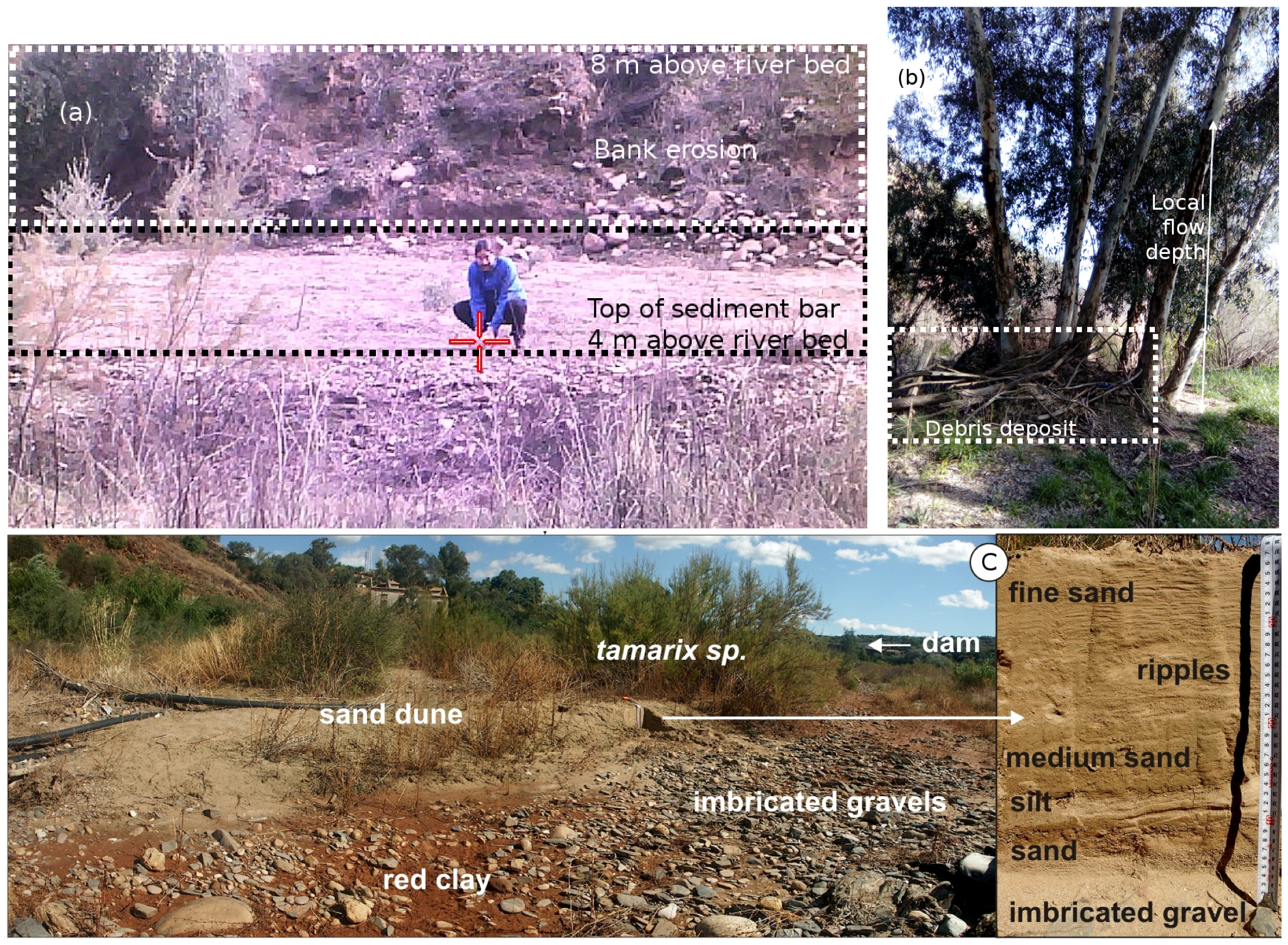
• The lack of bedforms and fine sediment deposits in the first river reach indicates a transport capacity larger than sediment supply. Only woody debris and a siltline are preserved at elevated bedrock terraces (9 m above the thalweg) or anthropogenic platforms (i.e., roads) below the dam. Surface gravel structures were formed by pebble to cobble grain-sized angular clasts. Downstream imbricated clasts support the argument of low sediment supply to sediment capacity ratio [59]. The high sediment transport capacity below the dam could be associated with the extreme turbulent intensity of the water down the spillways which was able to resuspend fine sediments [60].
• A field of sandy mud bumps developed on a bedrock bench further downstream. Bumps of cohesive mixtures of mud and sand are preserved downstream of flow obstacles (i.e., downstream flexible-wood trees such as Tamarix sp. and Fraxinus sp.). Shrubs on the bumps could initiate the accumulation of sediments as happens in obstacle dune. The bedforms resemble linear or long straight dunes. They are elongated along the longitudinal axis, being the width and height of the bumps much shorter than its longitudinal length.
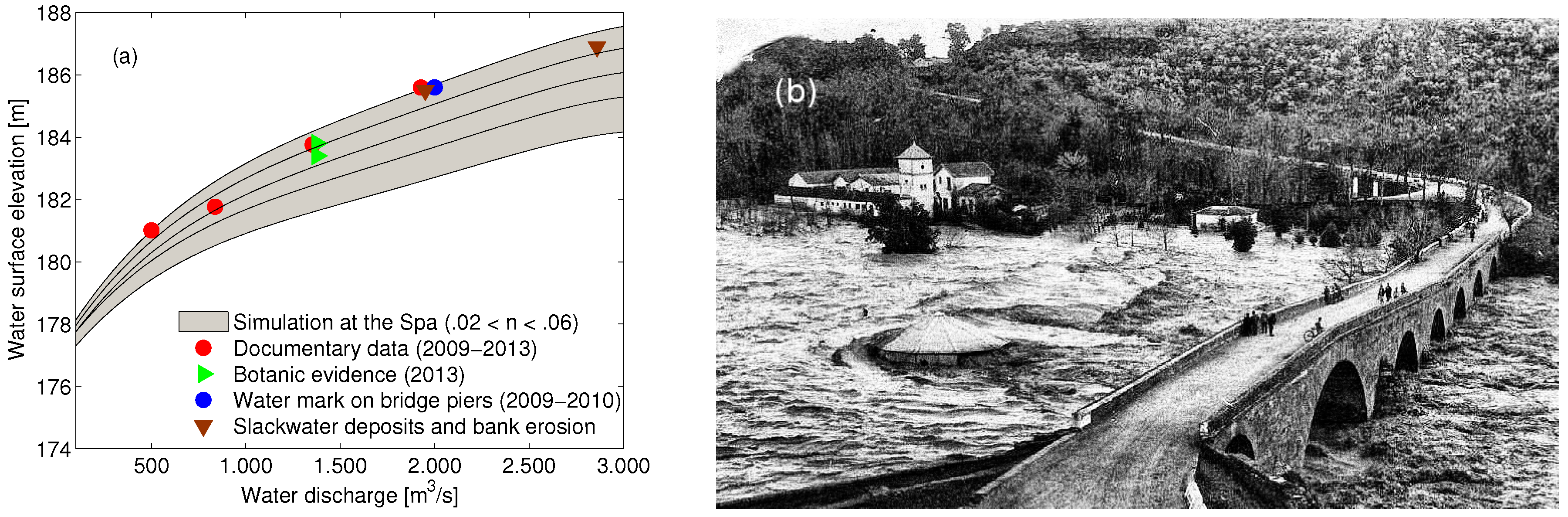
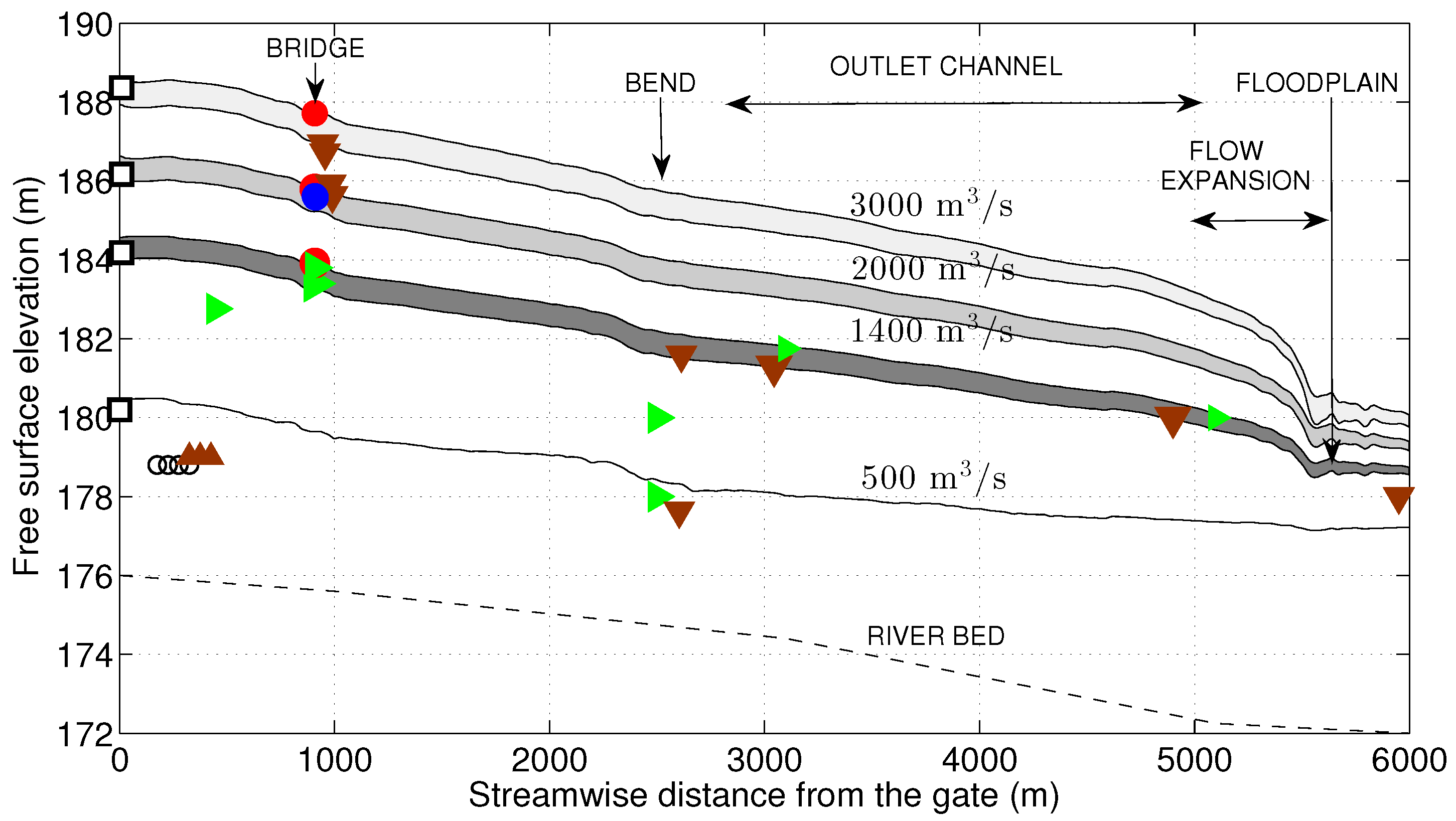
• Overbank flood-deposited sediments downstream of the bridge ($x\approx 1000$ m) was identified as a sedimentary evidence of flood level with the depth of 11 m. The documentary rating curve in Figure 3a indicates that the corresponding water discharge should be $Q\gg 2000$ m³$·$s⁻¹.
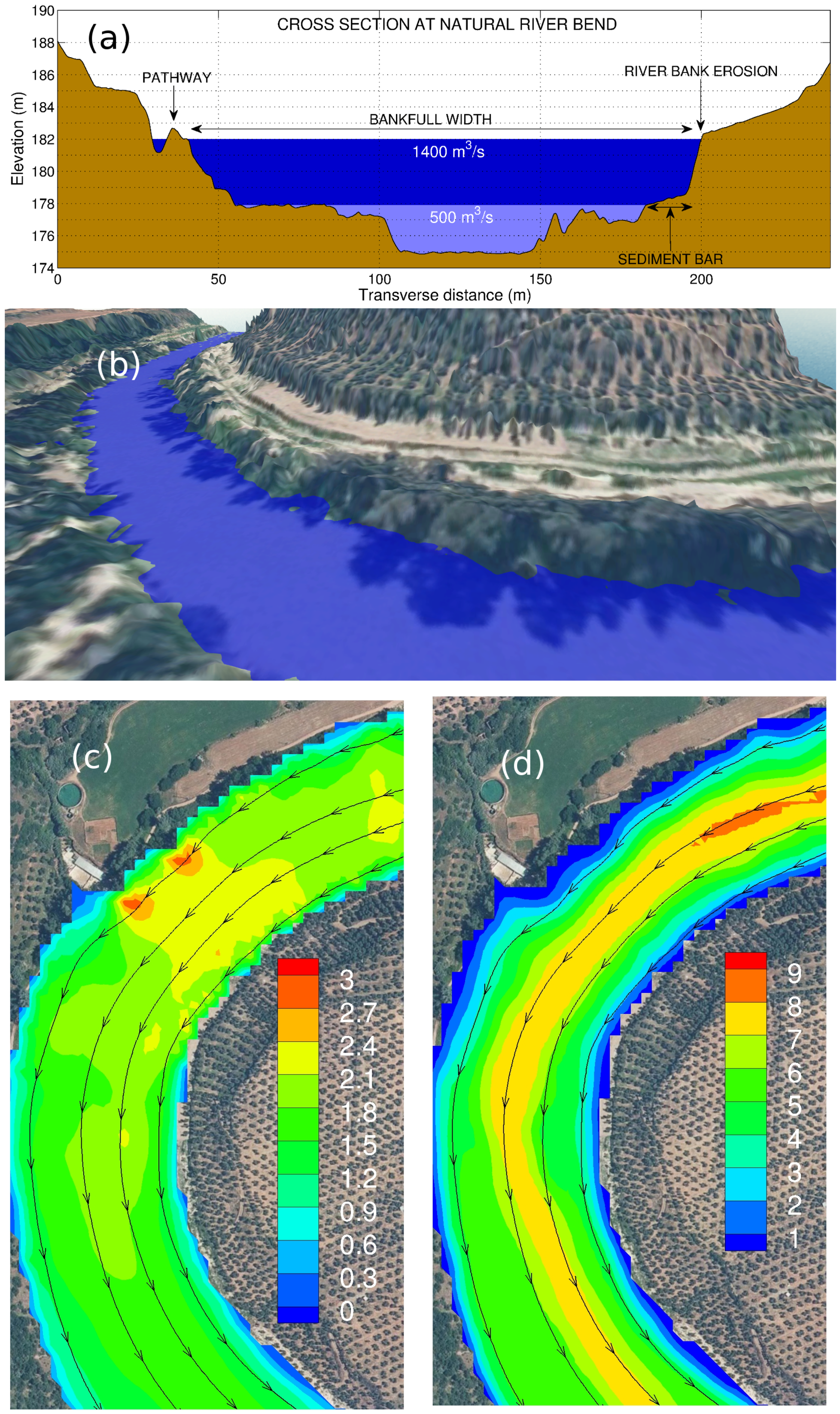
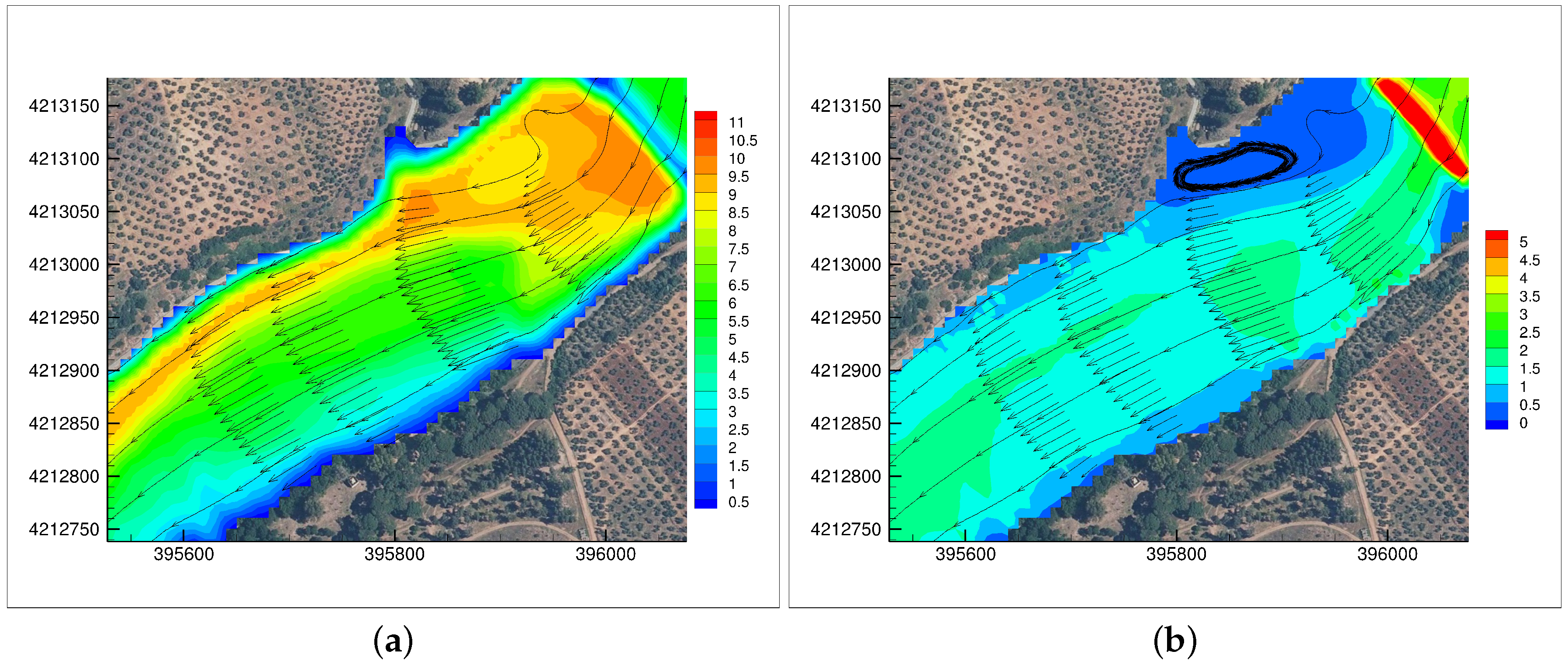
• Bank erosion also developed further downstream, on the inner side of the natural river bend ($x\approx 2500$ m). The photograph and the 3D representation of the bend shown in Figure 5a and Figure 7b, respectively, illustrate the lateral sediment bar that formed at the bottom of the inner bank. The elevation of the sediment bar measured during fieldworks (≈178 m) is in good agreement with the LiDAR data shown in Figure 7a. The top of the riverbanks at the bend (≈182 m) is elevated 8 m above the thalweg.
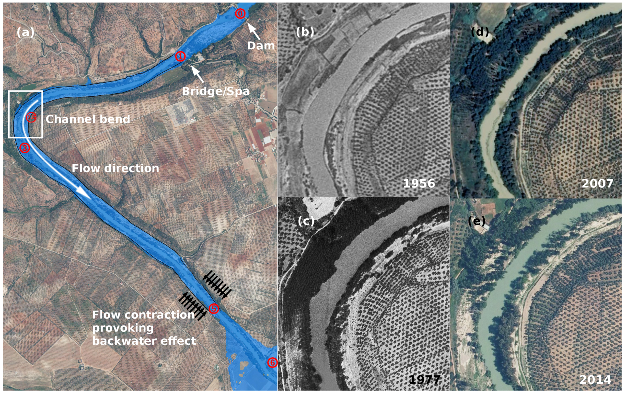
• Laterally-attached sandy siltlines were deposited from the end of the bend up to the flow expansion area ($3000<x<5000$ m) during the April 2013 flood. Their locations could be readily identified in the most recent orthophoto (see the solid line in black in Figure 4a) and the elevations could be inferred based on the LiDAR data. For the sake of the brevity, the elevations are shown in Figure 6 only at the beginning and at the end of the sediment deposits.
• Botanical HWMs are depicted with green right triangles in Figure 6. Figure 5b shows an illustrative example which was identified in the flow contraction area of the outlet channel (see location in Figure 4a). These botanical records are consistent with other flow stage indicators as the top level of lateral bars and imagery for the flood occurred in April 2013.

3.2. Calibration of the Numerical Model Pre- and Post-Vegetation Encroachment

The co-existence of gauging records during the periods 1910–1930 and 2009–2013 (Figure 2b) allowed the calibration of the numerical model in two situations: (i) pre-vegetation encroachment; and (ii) post-vegetation encroachment due to upstream impoundment. Woody species such as poplars, tamarisks and willows were really heterogeneous in the study area. Their state may also vary with seasons. Taking into account that the real characteristics of vegetation are unknown at the days of floodings, correlations of the friction factor for given tree dimensions and tree density could not be used in the modelling [50]. Calibration against measured rating curves at the foot of the dam is preferred in this occasion.

The Manning’s coefficient is commonly assumed uniform in paleohydrology [61] because the uncertainty associated with the non-uniformity of the roughness is negligible with respect to other factors (e.g., the true topography in older floods and the hydrograph shape in rapid-varying floods). Hence, numerical simulations were run for constant Manning’s values in the range of $0.02\le n\le 0.06$ s$·$m^−1/3 corresponding with a depth of flow reaching branches [62]. According to experimental observations, the free surface is horizontal in a fixed cross section. Numerical simulations (see Section 3.3) show that vegetation is homogeneous along the streamlines, although heterogeneous in the transversal direction. Subsequently, the assumption of a constant Manning’s roughness coefficient might induce some errors in the computation of the cross-section velocity profiles, which were avoided in the paleohydraulic reconstruction by using only PSI-HWMs well correlated with the flood stages.

Rating curves shown in Figure 2b at the foot of the dam were used to calibrate Manning’s roughness by comparing calculated stages to observed stages. The stage-discharge curve at the upstream boundary reflects the influence of riparian vegetation in the downstream channel of length >6 km because the flow regime is subcritical. Indeed there is a characteristic curve travelling upstream which propagates the physical information from the downstream channel to the inlet [63]. The shadow area in Figure 2b shows the stage-discharge curve obtained numerically. Comparison of numerical and experimental results serves to infer Manning’s value at a given discharge and point in time.

It was found that the Manning’s roughness of 0.02 s$·$m^−1/3 corresponds to moderate water discharges <1000 m³$·$s⁻¹ independently of the age of floods. Larger water discharges required higher friction factors up to 0.04 s$·$m^−1/3 for the oldest floods (1910–1930). The increase of the friction factor during flood mimics the effect of riparian vegetation on flow resistance and flood potential. Even higher friction factors were needed to simulate appropriately modern floods. Larger values of Manning’s coefficient were found out (up to 0.055 s$·$m^−1/3 for the water discharge of 2000 m³$·$s⁻¹) using the rating curve of 2009–2013 floods (red circles in Figure 2b). Verification of numerical results against hydrological data further downstream is presented in Section 3.3 and Figure 6.

To prove the existence of backwater effects in the problem at hand, the numerical rating curve corresponding with the numerical simulation of the shorter reach $0\le x\le 800$ m and the Manning’s coefficient of $n=0.02$ s$·$m^−1/3 was compared against actual results, see the dashed-dotted line in Figure 2b. The ensuing rating curve under-predicts the flow depth by a large extent (i.e., 2 m at 2500 m³$·$s⁻¹) with respect to previous numerical results, corroborating backwater effects at the channel outlet that affect the flood stages far upstream (recall Figure 4a).

This section concludes pointing out the accuracy of the numerical predictions at the reservoir. The dashed line in Figure 2b reproduces the trend of the gauging record (dots) particularly for water discharges higher than 500 m³$·$s⁻¹. Gates were operated at lower discharges. As gates were assumed open in the numerical simulation, recall Figure 2d,e, there is obviously a disparity between reality and simulation at low water discharge. Yet, the interest is the fluvial regime at flood stage and so this fact does not affect the analysis of larger water discharges.

3.3. Verification of the Simulated Floods with PSIs

Figure 6 represents the numerical results for the water discharges $Q=1400$, 2000 and 3000 m³$·$s⁻¹. These values correspond with inundations occurred in 2009–2013 (modern floods) and 1963 (historical flood). Taking into account that the PSI-HWMs described in Section 3.1 constrain the stages with an average error of $\pm 0.25$ m (equivalent to a Manning’s roughness uncertainty of $\pm 0.005$ s$·$m^−1/3), and using the mean roughness values given in Section 3.2, the Manning’s friction factor was set to 0.045 and 0.055 ± 0.005 s$·$m^−1/3 to simulate modern and historical floods, respectively. So numerical results in Figure 6 show the upper and lower bounds of the simulated water surfaces.

Independently of the water discharge, the shapes of the elevation profiles along the streamwise direction are qualitatively similar. Below the dam ($x<250$ m), the gradient of the water surface is very low. The three-dimensional representation of the numerical results (Figure 2d) readily illustrates this fact, in agreement with the observation of the February 2010 flood (Figure 2c). Further downstream, the free surface slope increases up to $0.1\%$ and remains nearly constant for $500\le x\le 4500$ m. So, the free surface slope is slightly larger than the average bed slope ($0.08\%$). For $x<4500$ m, if the water discharge varies, the water surface is translated vertically. For instance, the increases in discharge in the ranges of 1400–2000 m³$·$s⁻¹ and 2000–3000 m³$·$s⁻¹ lead to the increases in depth $1.84\pm 0.12$ m and $1.72\pm 0.12$ m, respectively. The free surface slope is much higher for $4500\le x\le 5500$ m due to the sudden expansion that occurs from the outlet channel in the confined valley to the floodplains, as shown in Figure 4a for $Q=1400$ m³$·$s⁻¹.

Although the water surface is flat near the dam ($0\le x\le 500$ m), the velocity field is non-uniform due to the development of a recirculation area below the powerhouse (Figure 8). The directions of the streamlines agree with the main axis of bumps in mixed sand-mud (Figure 5c). Flow depths and velocity magnitudes over the bumps vary in the ranges of 7–9 m and 1.5–2 m$·$s⁻¹, respectively, for $1400\le Q\le 2000$ m³·s⁻¹ but their correlation with bedform dimensions could not be addressed because of the nontransverse shape of bedforms, the non-uniformity of the flow field and the contrasting role of cohesive forces in flow and bed [64,65] which prevent the use of universal laws obtained in laboratory experiments under uniform and steady flow conditions [13,60].

Figure 3a and Figure 6 show an excellent agreement between simulations and retrodicted levels using imagery (red dots) at the bridge/Spa location ($x\approx 900$ m) for $Q=1400$ and 2000 m³$·$s⁻¹. Other indicators as HWMs at bridge piers, eroded riverbank levels and botanical evidence (scars on trees) are also in excellent agreement with numerical simulations. Watermarks at the bridge piers are associated with the February 2010 flood and the peak hourly average water discharge 1925 m³$·$s⁻¹. Probably, the instantaneous peak discharge was slightly larger which explains the good correlation with the simulation of 2000 m³$·$s⁻¹. Slackwater deposits at the rear of the bridge record the same water level and, consequently, are well correlated with $Q=2000$ m³$·$s⁻¹. The unique indicators of the most severe flood in the last century are overbank flood-deposited sediments downstream of the bridge. As a matter of fact, the paleohydraulic reconstruction shows that this sedimentological PSI is well correlated with the water discharge $Q=3000$ m³$·$s⁻¹ (17 February 1963). On the other hand, elevations of tree wounds (green right triangles) overlap with the level of the water discharge $Q=1400$ m³$·$s⁻¹. Scars on trees should have been developed during the most modern inundations (April 2013) with the hourly average peak water discharge of 1378 m³$·$s⁻¹. No botanical evidence in Figure 6 could be correlated with the simulated profiles for $2000\le Q\le 3000$ m³$·$s⁻¹. The absence of botanical marks for older, more severe floods corroborates their perishable nature [16].

In the downstream direction, the next hydrological evidence of interest appears at the natural river bend ($x\approx 2500$ m). On the one hand, the top of the eroded riverbank is as high as the simulated flood level for $Q=1400$ m³$·$s⁻¹ (see cross section in Figure 7a). The water surface elevation achieves approximately 182 m and the flow depth is 7 m. On the other hand, the sediment bar on the inner side of the bend is submerged 4 m below the water surface. The velocity field depicted in Figure 7c is really complex and non-uniform at this location, reaching a maximum of 3 m$·$s⁻¹ close to the outer riverbank and much lower values of 1.2 m$·$s⁻¹ in the lateral bar. In contrast, the free surface slope is as low as in the rest of the channel, leading to the flow depth field in Figure 7d. The sharp decrease in velocity near the inner bank should provoke the sedimentation of sand grains and the formation of the sediment bar. Interestingly, the streamlines (solid lines in Figure 7c) do not show flow separation. The elevation of woody debris in the outer floodplain is similar to the sediment bar elevation (see Figure 6). Sediments also settled over the outer floodplain, near the bend outlet, recall Figure 4e. Once again, slackwater deposits can be attributed to the sudden decrease in velocity magnitude at this location. The velocity magnitudes achieve values consistent with the simulated ones in the sediment bar, i.e., about 1.2 m$·$s⁻¹.

Laterally-attached sandy siltlines extended from the end of the river bend up to the flow expansion area ($3000<x<5000$ m). Their elevations are in excellent agreement with the numerical simulation with $Q=1400$ m³$·$s⁻¹ along the whole reach. Leaves debris at the branches of riparian trees, see Figure 5b, indicate the same flood levels as siltlines and numerical simulation. Slackwater deposits at the sudden expansion from the confined channel to the floodplain (denoted with a triangle symbol at $x\approx 6000$ m in Figure 6) poorly constrain the flood stage (i.e., flow depth increases only 1.5 m when the water discharge varies from 1400 to 3000 m³$·$s⁻¹). Floods previous to 2013 could not be identified at these locations because of soil management and the developments of the riparian vegetation cover. Anyway, the most recent flood served to verify the accuracy of the paleoflood reconstruction.

To conclude, it is worth pointing out the trend in flood stages over time that was observed in the numerical simulations. Current results demonstrate the spread of vegetation in regulated rivers provoking changes in the stage-discharge relationship over time that can be quantified by increasing the friction factor in the shallow water equations. In terms of water depth, vegetation encroachment led to 1 m deeper floods in 2009–2010 than in 1910–1930 for the same value of the water discharge $Q=2000$ m³$·$s⁻¹. Vegetation encroachment developed just after upstream river impoundment, between the years 1962 and 1977 (Figure 4), which yields 10% deeper floods and an increase of Manning’s roughness coefficient from 0.04 to 0.055 s$·$m^−1/3 in less than 15 years.

4. Conclusions

In this study, a wide collection of hydrological data including gauging records, imagery, botanical HWMs and sedimentary PSIs were used to reconstruct modern floods. Commonly, sedimentary sequences have been used in paleohydrology to reconstruct megafloods e.g., [1,5,6,7,8,10,24], historical floods [20,27] and glacial-lake outburst floods [2,3,4,25]. This study has shown that instrumental records and PSI-HWMs can be used together to check the accuracy of the 2D paleohydraulic reconstruction of recent floods in a well-gauged river.

The following conclusions can be drawn from the paleoflood reconstruction:

• Following Blocken and Gualtieri [30], high-quality experimental data are indispensable for the validation of any computational river dynamics model. Jarrett and England [14] showed that the elevation at the flood-deposited sediments nearest to channel margins provides a reliable and accurate indication of the maximum height of the flood. Hence, sedimentological HWMs can be used to check the accuracy and reliability of the 2D Saint-Venant equations in paleohydrology.
• Botanical HWMs provide valuable data for understanding recent floods and reconstructing their spatial patterns but botanical PSIs are perishable, might be washed out by more extreme floods and need to be preserved, as recently pointed out by Koenig et al. [16].
• Comparison with documentary data and imagery demonstrates that botanical and sedimentological HWMs, as well as mud-lines on man-made structures, are reliable data to indicate flood stages. Furthermore, the rating curve obtained from the combined use of 2D numerical simulations and imagery was nearly as accurate as gauging measurements.
• Overbank flood-deposited sediments are the only PSIs that record the most extreme flood. Interestingly, the simulated water depth of the largest flood in this study is much higher than in Jarrett and England’s [14] work (12 m vs. 4.5 m), and closely matches the observed flood stage, confirming previous findings on the reliability of PSI-HWMs for paleoflood studies.
• Dunes, imbricated pebbles and lateral bars are indirect indicators of the hydraulic conditions. Usually, flow depth and velocity magnitude for a given bedform dimension are deduced from dimensionless correlations under uniform and steady flow conditions [13,60]. However, PSIs are uncorrelated with these universal laws in non-uniform flows.

Lastly, the current paleoflood study shows that the long-term evolution of vegetation (>50 years) acts as a geomorphic driver of flood hazard through encroachment of the main channel, which supports recent results by Slater et al. [66] across many rivers in the USA. This novel application of paleohydrology could be used in other study sites that have experienced similar changes in the stage-discharge relationship in an age of climate extremes [67].

References

1. Baker, V.R. Paleoflood hydrology: Origin, progress, prospects. Geomorphology 2008, 101, 1–13. [Google Scholar] [CrossRef]
2. Carrivick, J.L. Application of 2D hydrodynamic modelling to high–magnitude outburst floods: An example from Kverkfjöll, Iceland. J. Hydrol. 2006, 321, 187–199. [Google Scholar] [CrossRef]
3. Bohorquez, P.; Darby, S.E. The use of one– and two–dimensional hydraulic modelling to reconstruct a glacial outburst flood in a steep Alpine valley. J. Hydrol. 2008, 361, 240–261. [Google Scholar] [CrossRef]
4. Westoby, M.J.; Glasser, N.F.; Brasington, J.; Hambrey, M.J.; Quincey, D.J.; Reynolds, J.M. Modelling outburst floods from moraine-dammed glacial lakes. Earth-Sci. Rev. 2014, 134, 137–159. [Google Scholar] [CrossRef]
5. Baker, V.R.; Benito, G.; Rudoy, A.N. Paleohydrology of late Pleistocene superflooding, Altay Mountains, Siberia. Science 1993, 259, 348–350. [Google Scholar] [CrossRef] [PubMed]
6. Herget, J. Reconstruction of Pleistocene ice-dammed lake outburst floods in the Altai Mountains, Siberia. Spec. Pap. Geol. Soc. Am. 2005, 386, 1–118. [Google Scholar]
7. Carling, P.A.; Villanueva, I.; Herget, J.; Wright, N.; Borodavko, P.; Morvan, H. Unsteady 1D and 2D hydraulic models with ice dam break for Quaternary megaflood, Altai Mountains, southern Siberia. Glob. Planet. Chang. 2010, 70, 24–34. [Google Scholar] [CrossRef]
8. Bohorquez, P.; Carling, P.A.; Herget, J. Dynamic simulation of catastrophic late Pleistocene glacial-lake drainage, Altai Mountains, central Asia. Int. Geol. Rev. 2016, 58, 1795–1817. [Google Scholar] [CrossRef]
9. Benito, G.; Lang, M.; Barriendos, M.; Llasat, M.; Francés, F.; Ouarda, T.; Thorndycraft, V.R.; Enzel, Y.; Bardossy, A.; Coeur, D.; et al. Use of systematic, palaeoflood and historical data for the improvement of flood risk estimation. Review of scientific method. Nat. Hazards 2004, 31, 623–643. [Google Scholar]
10. Baker, V.R. Paleoflood hydrology and extraordinary flood events. J. Hydrol. 1987, 96, 79–99. [Google Scholar] [CrossRef]
11. Lumbroso, D.; Gaume, E. Reducing the uncertainty in indirect estimates of extreme flash flood discharges. J. Hydrol. 2012, 414–415, 16–30. [Google Scholar] [CrossRef]
12. Bohorquez, P.; García-García, F.; Pérez-Valera, F.; Martínez-Sánchez, C. Unsteady two–dimensional paleohydraulic reconstruction of extreme floods over the last 4000 yr in Segura River, southeast Spain. J. Hydrol. 2013, 447, 229–239. [Google Scholar] [CrossRef]
13. Carling, P.A. Freshwater megaflood sedimentation: What can we learn about generic processes? Earth Sci. Rev. 2013, 125, 87–113. [Google Scholar] [CrossRef]
14. Jarrett, R.D.; England, J.F. Reliability of paleostage indicators for paleoflood studies. In Ancient Floods, Modern Hazards; House, P.K., Ebb, R.H., Baker, V.R., Levish, D.R., Eds.; Water Science and Application; American Geophysical Union: Washington, DC, USA, 2002; pp. 91–109. [Google Scholar]
15. Carling, P.A.; Burr, D.M.; Johnsen, T.F.; Brennand, T.A. A review of open-channel megaflood depositional landforms on Earth and Mars. In Megaflooding on Earth and Mars; Burr, D., Carling, P.A., Baker, V.R., Eds.; Cambridge University Press: Cambridge, UK, 2009; pp. 33–49. [Google Scholar]
16. Koenig, T.A.; Bruce, J.L.; O’Connor, J.; McGee, B.D.; Holmes, R.R., Jr.; Hollins, R.; Forbes, B.T.; Kohn, M.S.; Schellekens, M.; Martin, Z.W.; et al. Identifying and preserving high-water mark data. U.S. Geol. Surv. Tech. Methods 2016. [Google Scholar] [CrossRef]
17. Brázdil, R.; Kundzewicz, Z.W.; Benito, G. Historical hydrology for studying flood risk in Europe. Hydrol. Sci. J. 2006, 51, 739–764. [Google Scholar] [CrossRef]
18. Hall, J.; Arheimer, B.; Borga, M.; Brázdil, R.; Claps, P.; Kiss, A.; Kjeldsen, T.R.; Kriauciuniene, J.; Kundzewicz, Z.W.; Lang, M.; et al. Understanding flood regime changes in Europe: A state-of-the-art assessment. Hydrol. Earth Syst. Sci. 2014, 18, 2735–2772. [Google Scholar] [CrossRef] [Green Version]
19. Kjeldsen, T.R.; Macdonald, N.; Lang, M.; Mediero, L.; Albuquerque, T.; Bogdanowicz, E.; Brzdil, R.; Castellarin, A.; David, V.; Flei, A.; et al. Documentary evidence of past floods in Europe and their utility in flood frequency estimation. J. Hydrol. 2014, 517, 963–973. [Google Scholar] [CrossRef] [Green Version]
20. Benito, G.; Brázdil, R.; Herget, J.; Machado, M.J. Quantitative historical hydrology in Europe. Hydrol. Earth Syst. Sci. 2015, 19, 3517–3539. [Google Scholar] [CrossRef]
21. Toonen, W.H.J.; Middelkoop, H.; Konijnendijk, T.Y.M.; Macklin, M.G.; Cohen, K.M. The influence of hydroclimatic variability on flood frequency in the Lower Rhine. Earth Surf. Process. Landf. 2016, 41, 1266–1275. [Google Scholar] [CrossRef]
22. Denlinger, R.P.; O’Connell, D.R.H.; House, P.K. Robust determination of stage and discharge: An example from an extreme flood on the Verde River, Arizona. In Ancient Floods, Modern Hazards; House, P.K., Ebb, R.H., Baker, V.R., Levish, D.R., Eds.; Water Science and Application; American Geophysical Union: Washington, DC, USA, 2002; pp. 127–146. [Google Scholar]
23. Alho, P.; Baker, V.R.; Smith, L.N. Paleohydraulic reconstruction of the largest Glacial Lake Missoula draining(s). Quat. Sci. Rev. 2010, 29, 3067–3078. [Google Scholar] [CrossRef]
24. Denlinger, R.P.; O’Connell, D.R.H. Simulations of cataclysmic outburst floods from Pleistocene glacial lake Missoula. Bull. Geol. Soc. Am. 2010, 122, 678–689. [Google Scholar] [CrossRef]
25. Winsemann, J.; Alho, P.; Laamanen, L.; Goseberg, N.; Lang, J.; Klostermann, J. Flow dynamics, sedimentation and erosion of glacial lake outburst floods along the Middle Pleistocene Scandinavian Ice Sheet (northern central Europe). Boreas 2016, 45, 260–283. [Google Scholar] [CrossRef]
26. Feldman, A.D. HEC models for water resources system system simulation: theory and experience. Adv. Hydrosci. 1981, 12, 297–423. [Google Scholar]
27. Herget, J.; Roggenkamp, T.; Krell, M. Estimation of peak discharges of historical floods. Hydrol. Earth Syst. Sci. 2014, 18, 4029–4037. [Google Scholar] [CrossRef] [Green Version]
28. Couderc, F.; Madec, R.; Martin, N.; Monnier, J.; Vila, J.P.; Dartus, D.; Honnorat, M.; Marin, J. DassFlow: Data Assimilation for Free Surface Flows. Available online: http://www-gmm.insa-toulouse.fr/∼monnier/DassFlow (accessed on 1 September 2014).
29. Monnier, J.; Couderc, F.; Dartus, D.; Larnier, K.; Madec, R.; Vila, J.P. Inverse algorithms for 2D shallow water equations in presence of wet dry fronts. Application to flood plain dynamics. Adv. Water Res. 2016, 97, 11–24. [Google Scholar] [CrossRef]
30. Blocken, B.; Gualtieri, C. Ten iterative steps for model development and evaluation applied to Computational Fluid Dynamics for Environmental Fluid Mechanics. Environ. Model. Softw. 2012, 33, 1–22. [Google Scholar] [CrossRef]
31. Darby, S.E. Effect of riparian vegetation on flow resistance and flood potential. J. Hydraul. Eng. 1999, 125, 443–454. [Google Scholar] [CrossRef]
32. Sanders, B.F. Evaluation of on-line DEMs for flood inundation modeling. Adv. Water Resour. 2007, 30, 1831–1843. [Google Scholar] [CrossRef]
33. Blayo, E.; Debreu, L. Revisiting open boundary conditions from the point of view of characteristic variables. Ocean Model. 2005, 9, 231–252. [Google Scholar] [CrossRef]
34. Barredo, J.; Saurand, D.; Llasat, M. Assessing trends in insured losses from floods in Spain 1971–2008. Nat. Hazards Earth Syst. Sci. 2012, 12, 1723–1729. [Google Scholar] [CrossRef] [Green Version]
35. Benito, G.; Machado, M.J. Floods in the Iberian Peninsula. In Changes in Flood Risk in Europe; IAHS Special Publication 10; Kundzewicz, Z.W., Ed.; IAHS Press and CRC Press/Balkema: Wallingford, UK, 2012; pp. 372–383. [Google Scholar]
36. Instituto Geológico y Minero de España (IGME). Análisis del Impacto de los Riegos Geológicos en España. Evaluación de Pérdidas por Terremotos e Inundaciones en el Periodo 1987–2001 y Estimación Para el Periodo 2004–2033; Instituto Geológico y Minero de España (IGME), Ministerio de Educación y Ciencia, Consorcio de Compensación de Seguros: Madrid, Spain, 2004. [Google Scholar]
37. Gilbert, G.K. The transportation of débris by running water. U.S. Geol. Surv. Prof. Pap. 1914, 86, 263. [Google Scholar]
38. Baker, V.R.; Kale, V.S. The role of extreme floods in shaping bedrock channels. In Rivers over Rock: Fluvial Processes in Bedrock Channels; Tinkler, K.J., Wohl, E.E., Eds.; American Geophysical Union: Washington, DC, USA, 1998; pp. 153–165. [Google Scholar]
39. Church, M. Bed material transport and the morphology of alluvial river channels. Annu. Rev. Earth Planet. Sci. 2006, 34, 325–354. [Google Scholar] [CrossRef]
40. Buffington, J.M.; Montgomery, D.R. Geomorphic classification of rivers. In Treatise on Geomorphology; Shroder, J., Wohl, E., Eds.; Fluvial Geomorphology; Academic Press: San Diego, CA, USA, 2013; Volume 9, pp. 730–767. [Google Scholar]
41. Davidian, J. Computation of Water Surface Profiles in Open Channels; USGS TWRI Book 3: Application of Hydraulics. Ch. A15; United States Geological Survey: Washington, DC, USA, 1984.
42. Vannéy, J.R. L’hydrologie du bas Guadalquivir; Consejo Superior de Investigaciones Científicas: Madrid, Spain, 1970. [Google Scholar]
43. Sistema de Información del Anuario de Aforos. Available online: http://sig.magrama.es/aforos (accessed on 1 September 2015).
44. Sistema Automático de Información Hidrológica de la Cuenca del Guadalquivir. Available online: http://www.chguadalquivir.es/saih/ (accessed on 1 September 2015).
45. Pascual, G.; Bustamante, A. Catálogo Nacional de Inundaciones Históricas. Actualización; Nipo: 126-11-150-1; Ministerio del Interior: Madrid, Spain, 2011. [Google Scholar]
46. Uribelarrea, D.; Benito, G. Fluvial changes of the Guadalquivir river during the Holocene in Córdoba (Southern Spain). Geomorphology 2008, 100, 14–31. [Google Scholar] [CrossRef]
47. Borja Palomo, F.D. Memoria Histórico-Crítico Sobre las Riadas o Grandes Avenidas del Guadalquivir en Sevilla, Desde Principio del Siglo XV hasta Nuestros días; Excmo. Ayto de Sevilla: Sevilla, Spain, 1877. [Google Scholar]
48. Infraestructura de Datos Espaciales de Andalucía. Available online: http://www.ideandalucia.es/IDEAvisor (accessed on 1 September 2015).
49. Bohorquez, P.; Aranda, V.; Calero, J.; García-García, F.; Ruiz-Ortiz, P.; Fernández, T.; Salazar, C. Floods in the Guadalquivir River (Southern Spain). In Proceedings of the International Conference on Fluvial Hydraulics, RIVER FLOW 2014, Lausanne, Switzerland, 3–5 September 2014; Schleiss, A., Cesare, G., Franca, M., Pfister, M., Eds.; CRC Press/Balkema: Leiden, The Netherlands, 2014; pp. 1711–1719. [Google Scholar]
50. Wu, W. Computation River Dynamics; Taylor & Francis: London, UK, 2007. [Google Scholar]
51. Courant, R.; Friedrichs, K.; Lewy, H. On the partial difference equations of mathematical physics. IBM J. Res. Dev. 1967, 11, 215–234. [Google Scholar] [CrossRef]
52. Plan Nacional de Ortofotografía Aérea, Instituto Geográfico Nacional de España. Available online: http://www.ign.es/PNOA (accessed on 1 September 2014).
53. Huang, W.; Cao, Z.X.; Carling, P.A.; Pender, G. Coupled 2D hydrodynamic and sediment transport modelling of megaflood due to glacier dam-break in Altai Mountains, Southern Siberia. J. Mt. Sci. 2014, 11, 1442–1453. [Google Scholar] [CrossRef]
54. Guan, M.; Wright, N.; Sleigh, P.; Carrivick, J. Assessment of hydro-morphodynamic modelling and geomorphological impacts of a sediment-charged jökulhlaup, at Sólheimajökull, Iceland. J. Hydrol. 2015, 530, 336–349. [Google Scholar] [CrossRef]
55. Bohorquez, P.; Ancey, C. Particle diffusion in non-equilibrium bedload transport simulations. Appl. Math. Model. 2016, 40, 7474–7492. [Google Scholar] [CrossRef]
56. Heyman, J.; Bohorquez, P.; Ancey, C. Entrainment, motion and deposition of coarse particles transported by water over a sloping mobile bed. J. Geophys. Res. Earth Surf. 2016, 121, 1931–1952. [Google Scholar] [CrossRef]
57. Alho, P.; Aaltonen, J. Comparing a 1D hydraulic model with a 2D hydraulic model for the simulation of extreme glacial outburst floods. Hydrol. Process. 2008, 22, 1537–1547. [Google Scholar] [CrossRef]
58. Petts, G.E. Long-term consequences of upstream impoundment. Environ. Conserv. 1980, 7, 325–332. [Google Scholar] [CrossRef]
59. Hassan, M.; Church, M. Experiments on surface structure and partial sediment transport on a gravel bed. Water Resour. Res. 2000, 36, 1885–1895. [Google Scholar] [CrossRef]
60. Yalin, M.S.; da Silva, A.M.F. Fluvial Processes; IAHR Monograph, IAHR: Delft, The Netherlands, 2001. [Google Scholar]
61. O’Connor, J.E.; Webb, R.H. Hydraulic modeling for paleoflood analysis. In Flood Geomorphology; Baker, V.R., Kochel, R.C., Patton, P.C., Eds.; John Wiley and Sons: New York, NY, USA, 1988; pp. 393–402. [Google Scholar]
62. Arcement, G.J., Jr.; Schneider, V.R. Guide for Selecting Manning’s Roughness Coefficients for Natural Channels and Flood Plains; U.S. Geological Survey Water-Supply Paper; United States Government Printing Office: Denver, CO, USA, 1989; Volume 2339.
63. Whitham, G.B. Linear and Nonlinear Waves; John Wiley & Sons: New York, NY, USA, 1974. [Google Scholar]
64. Baas, J.H.; Davies, A.G.; Malarkey, J. Bedform development in mixed sand-mud: The contrasting role of cohesive forces in flow and bed. Geomorphology 2013, 182, 19–32. [Google Scholar] [CrossRef]
65. Baas, J.H.; Best, J.L.; Peakall, J. Predicting bedforms and primary current stratification in cohesive mixtures of mud and sand. J. Geol. Soc. 2015. [Google Scholar] [CrossRef]
66. Slater, L.J.; Singer, M.B.; Kirchner, J.W. Hydrologic versus geomorphic drivers of trends in flood hazard. Geophys. Res. Lett. 2015, 42, 2014GL062482. [Google Scholar] [CrossRef]
67. Naylor, L.A.; Spencer, T.; Lane, S.N.; Darby, S.E.; Magilligan, F.J.; Macklin, M.G.; Möller, I. Stormy Geomorphology: Geomorphic contributions in an age of climate extremes. Earth Surf. Process. Landf. 2016. [Google Scholar] [CrossRef]
Figure 1. Digital elevation model of the study site showing the Guadalquivir River in the confined valley that connects the floodplains upstream and downstream of the Marmolejo dam (N 38 3 31 E 4 11 13 ). The drainage area of the Guadalquivir River Basin upstream of the dam is 19,546 km2. The characteristic dimensions of the dam are: height = 20 m, crest length = 230 m, spillway crest = 186.2 m, top of tainter gate = 191.73 m, outlet channel elevation = 175.35 m, reservoir capacity = 13 Hm3 and design flood = 3450 m3 · s−1.
Water 08 00567 g001
Figure 2. (a) Flood frequency distribution and relative magnitude of the Guadalquivir river instrumental floods at Marmolejo dam; (b) Rating curve upstream and downstream of the dam; (c) Flooded area below Marmolejo dam on 24 February 2010 for Q = 1847 m3 · s−1. The distance between the old and new hydropower is nearly the same as the length of the dam, i.e., 195 m; (d) Detail of the water surface elevation; and (e) the computational mesh as for panel (c) with Q = 1900 m3 · s−1 and n = 0 . 06 s · m−1/3. The grid resolution is <1 m at the spillways and progressively coarser (<10 m) over the valley. The simulated water surface is nearly flat (vanishing free surface slope) few meters downstream of the dam in agreement with observations in panel (c). Note the similarity between the modelled hydraulic structure and the real one as well as the modelled and observed inundated areas.
Water 08 00567 g002
Figure 3. (a) Rating curve at the bridge/Spa based on in situ photographs during 2009–2013 floods, botanical high-water marks (HWMs), mud-lines on bridge piers and overbank flood-deposited sediments; (b) Flooded area on 18 February 1963 when the flow rate was 2200 m3 · s−1.
Water 08 00567 g003
Figure 4. (a) Blue colour represents the inundated area obtained in the numerical simulation for the water discharge Q = 1400 m3 · s−1 with Manning’s coefficient n = 0 . 05 s · m−1/3. Numbers show the location and the distance to the dam (in km) of the main paleostage indicators (PSIs). The black lines highlight the slackwater deposits of fine sediments found out along the riversides in fieldworks as well as in the 2014 orthophoto; (be) Sequence of orthophotos in the bend (white box in panel (a)) showing the states before/after river regulation (1956/1977) and snapshots before/after modern floods (2007/2014). Note the absence of riparian vegetation in 1956 (panel (b)), the proliferation of riparian vegetation after river regulation (panel (c)) which started in 1962 with Marmolejo dam and prevails up to present days (panels (d,e)), and the presence of slackwater deposits in 2014 (panel (e)) as a consequence the April 2013 flood.
Water 08 00567 g004
Figure 5. (a) Snapshot acquired with Leica DISTOTM S910 during the positioning of the top of the lateral bar in the river bend (square box in Figure 4a); (b) Botanical evidence in the left bank of the hydraulic control reach: it is located within the contraction area depicted in Figure 4a. The highest watermark in the tree (8 m above the thalweg) was used as botanical evidence establishing the water level of ∼180 m at x = 5100 m; (c) Sand dune downstream a tamarisk tree and sedimentological sequence of the internal organisation of the sand dune.
Water 08 00567 g005
Figure 6. Streamwise profile of the simulated water surfaces for the flow discharges: 500 ( n = 0 . 02 s · m−1/3), 1400 ( 0 . 04 n 0 . 05 s · m−1/3), 2000 and 3000 m3 · s−1 ( 0 . 05 n 0 . 06 s · m−1/3). The dotted line represents the thalweg profile. Symbols correspond with the PSIs in Figure 2b and Figure 3a, except empty circles and upward triangles which represent pebbles and dunes, respectively.
Water 08 00567 g006
Figure 7. (a) Characteristic cross section at the natural river bend shown in Figure 4b–d. Flood levels for Q = 500 and 1400 m3 · s−1 are depicted in light and dark blue, respectively; (b) 3D view of the river bend (base flow level =175 m) and sediment bar shown in Figure 5a. Panels (c,d) show simulated values of the velocity magnitude (m · s−1) and the flow depth (m) with Q = 1400 m3 · s−1, respectively.
Water 08 00567 g007
Figure 8. Details of the simulated (a) flow depth; and (b) velocity magnitude from the dam to the Spa ( x 775 m) with Q = 1400 m3 · s−1. Representative streamlines and velocity vectors are also depicted.
Water 08 00567 g008