
A Methodology for the Optimization of Flow Rate Injection to Looped Water Distribution Networks through Multiple Pumping Stations

 ,
,  and
and
Abstract
:1. Introduction
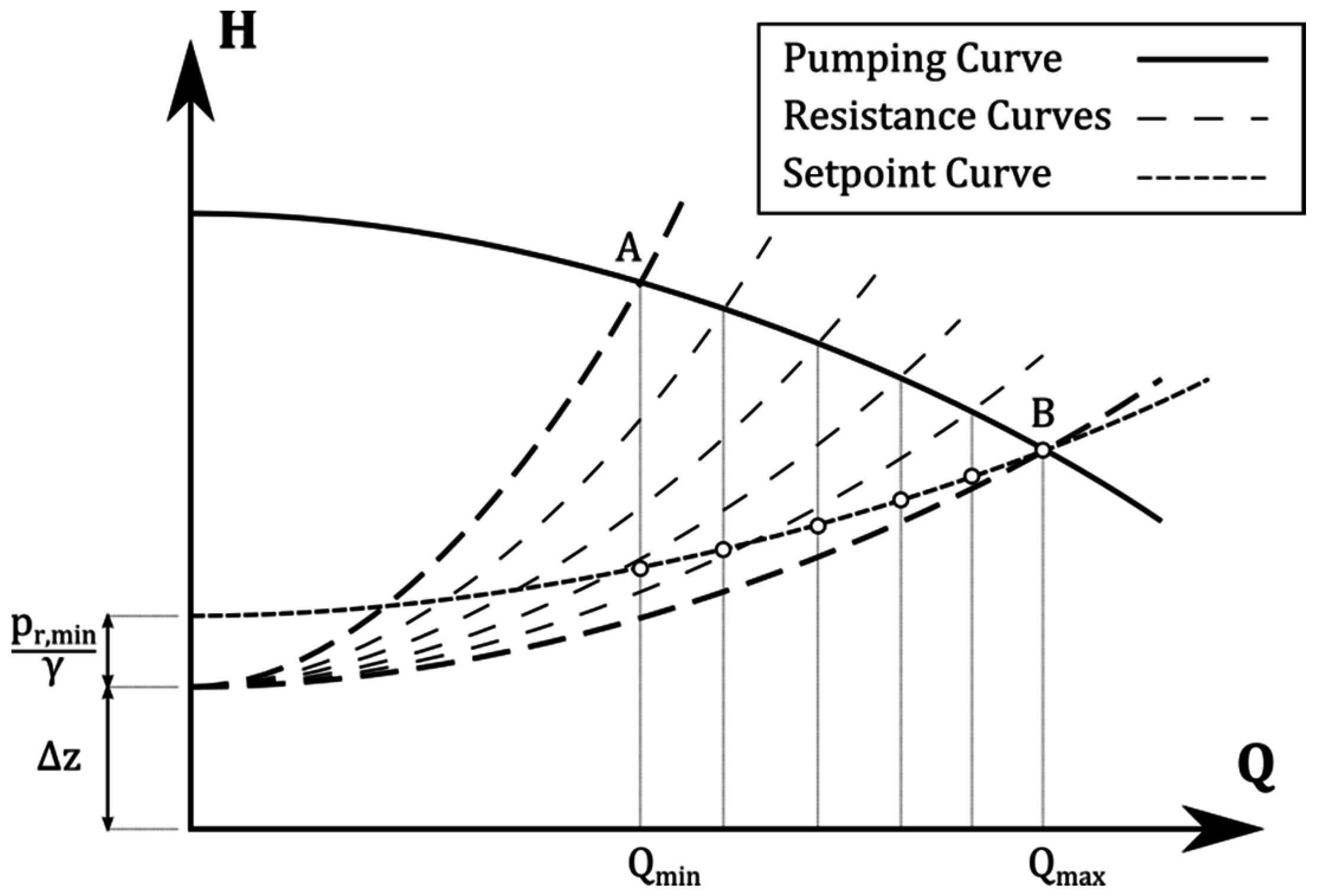
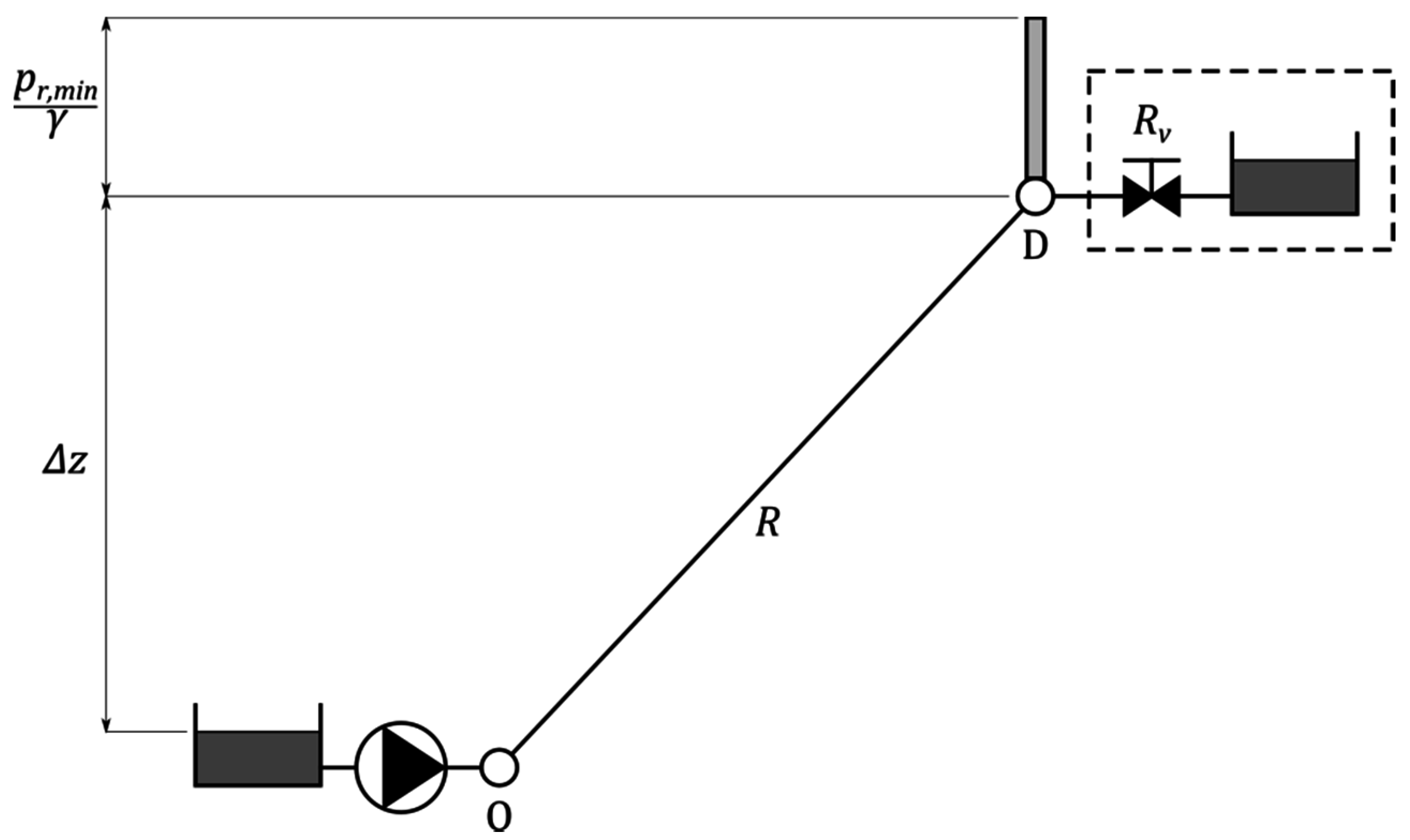
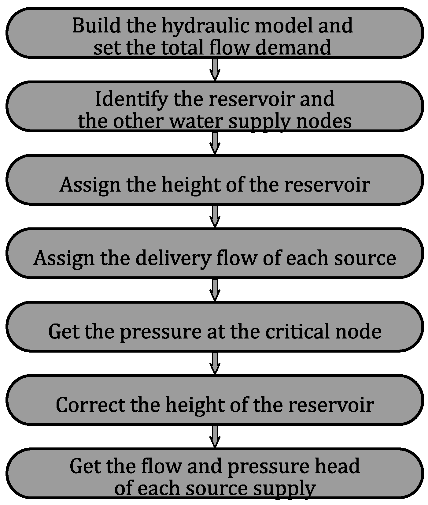
2. Setpoint Curve
3. Optimization Function
- The total flow fed into the network system from all sources must equal the total flow rate demanded on stage (j).
- The flow rate supplied for each source will be as low as 0 and as high as the total flow rate demands.
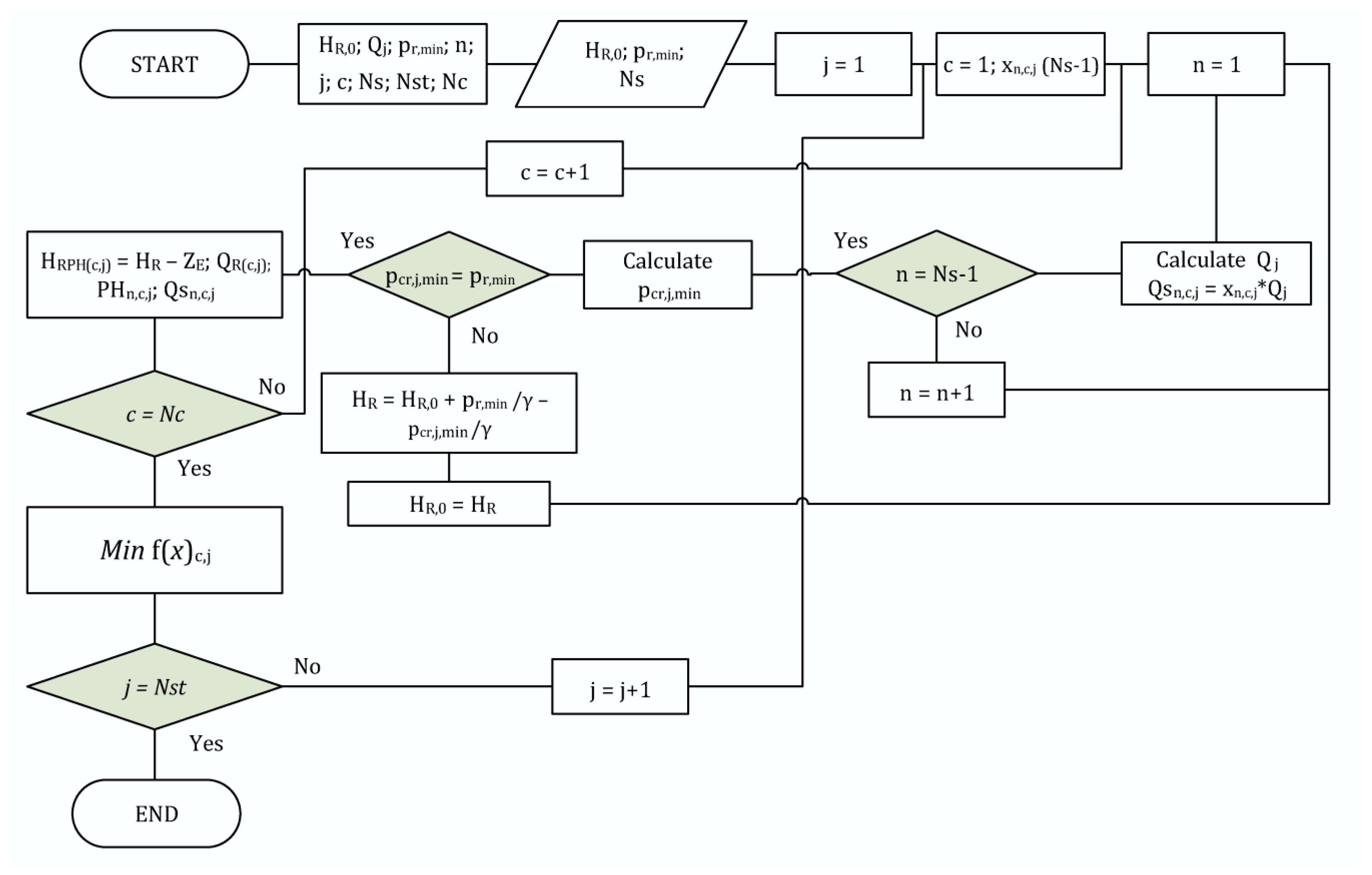
3.1. Discrete Method
3.2. Continuous Method
3.2.1. The Hooke–Jeeves Algorithm
3.2.2. The Nelder–Mead Algorithm
4. Case Studies
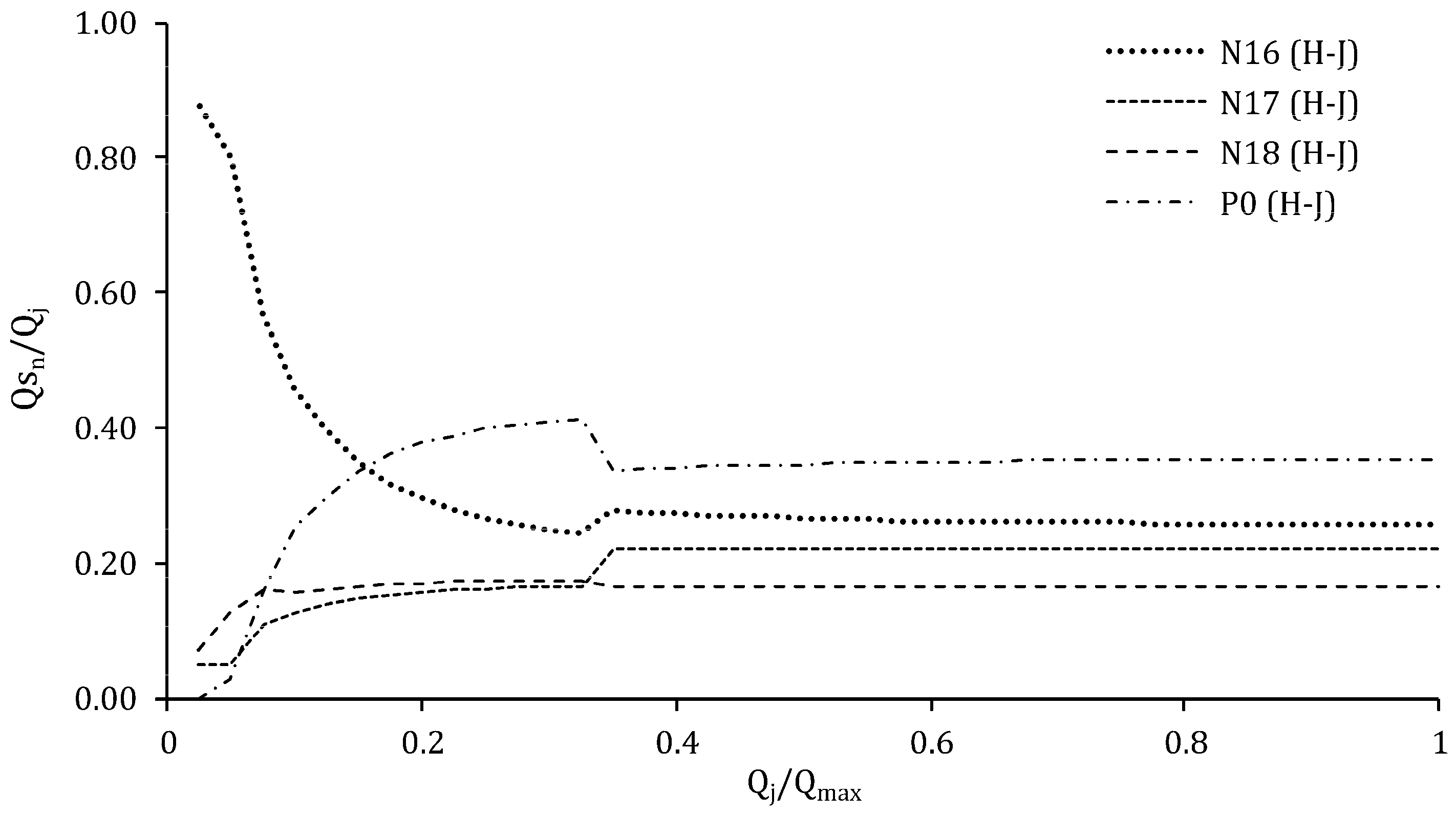
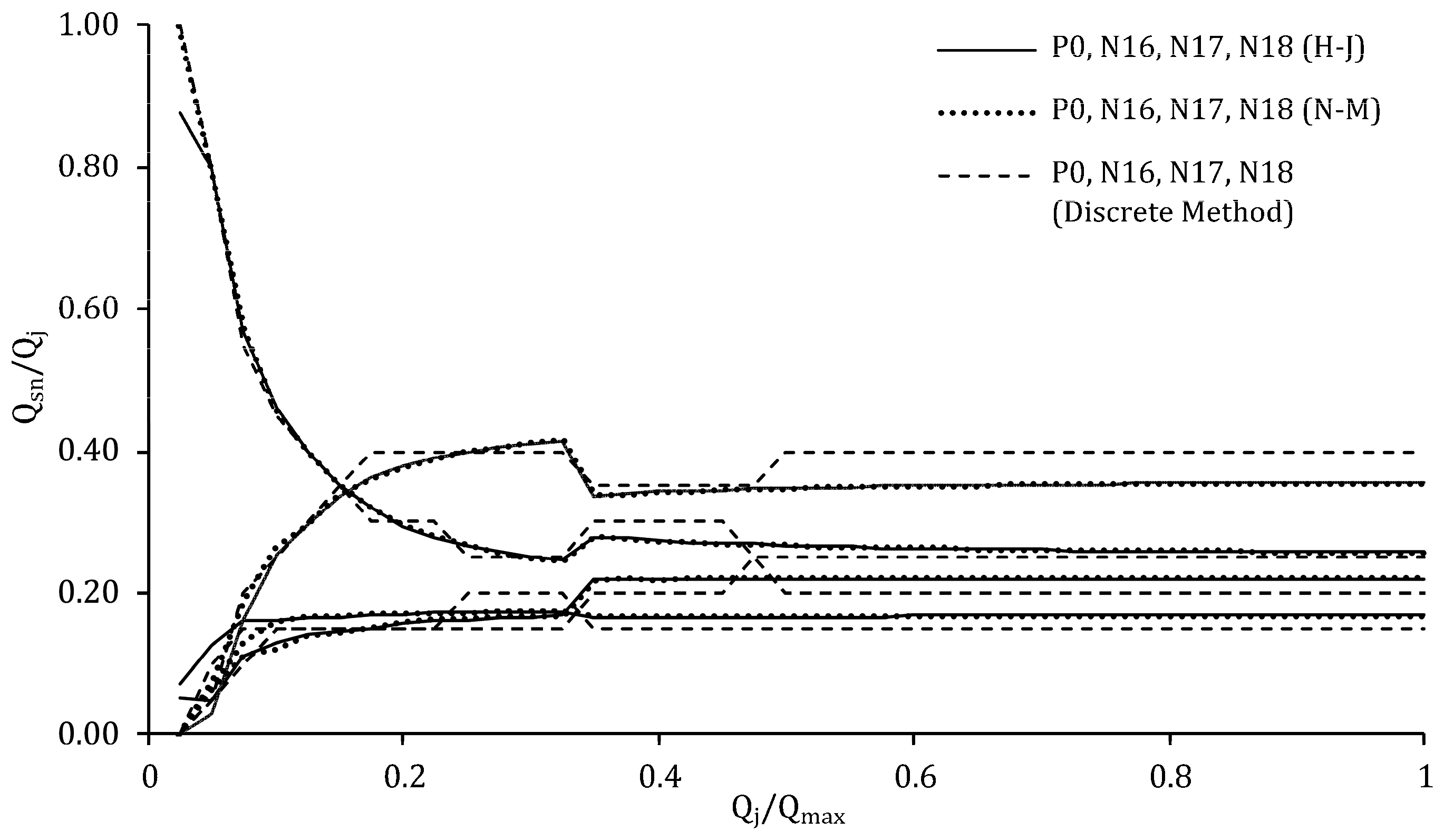
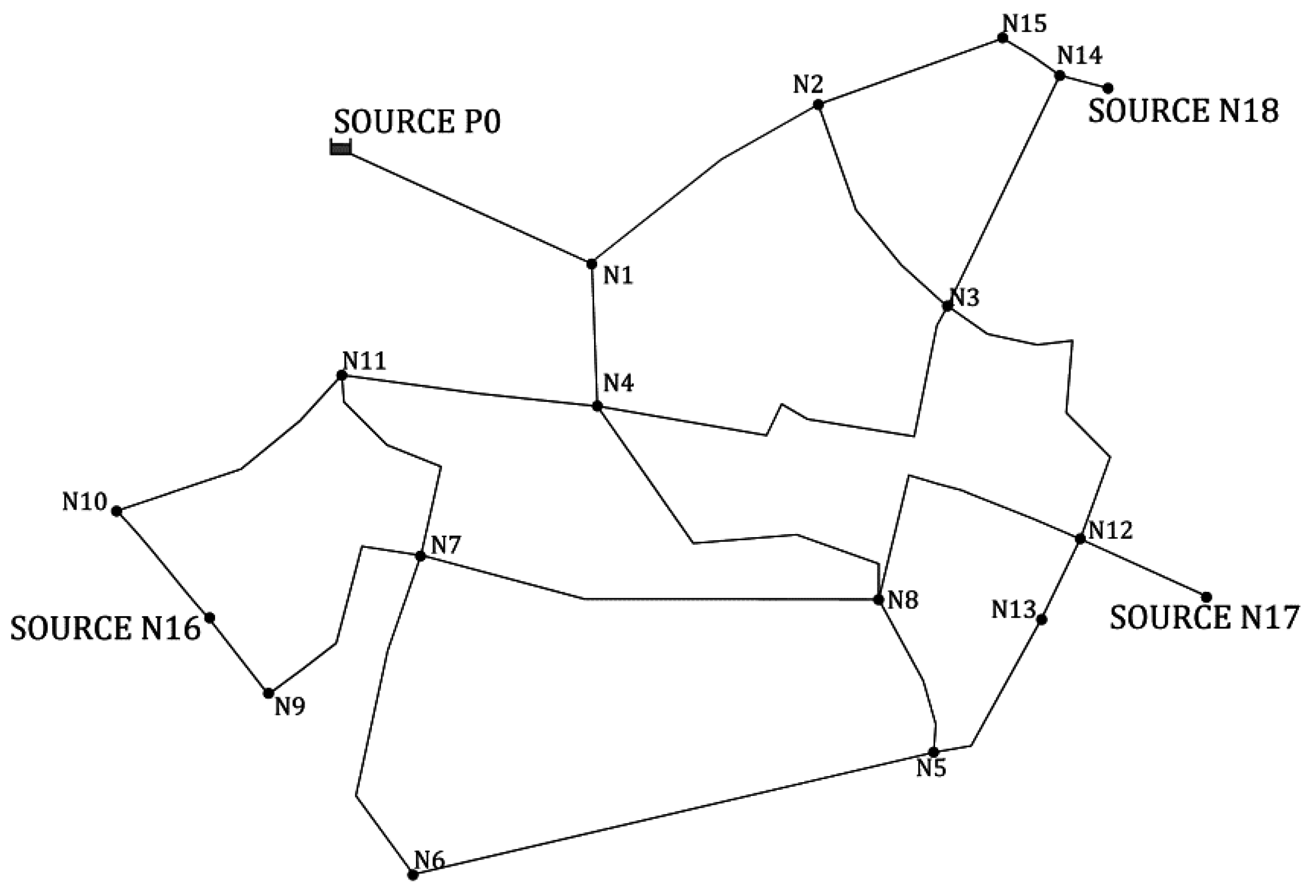
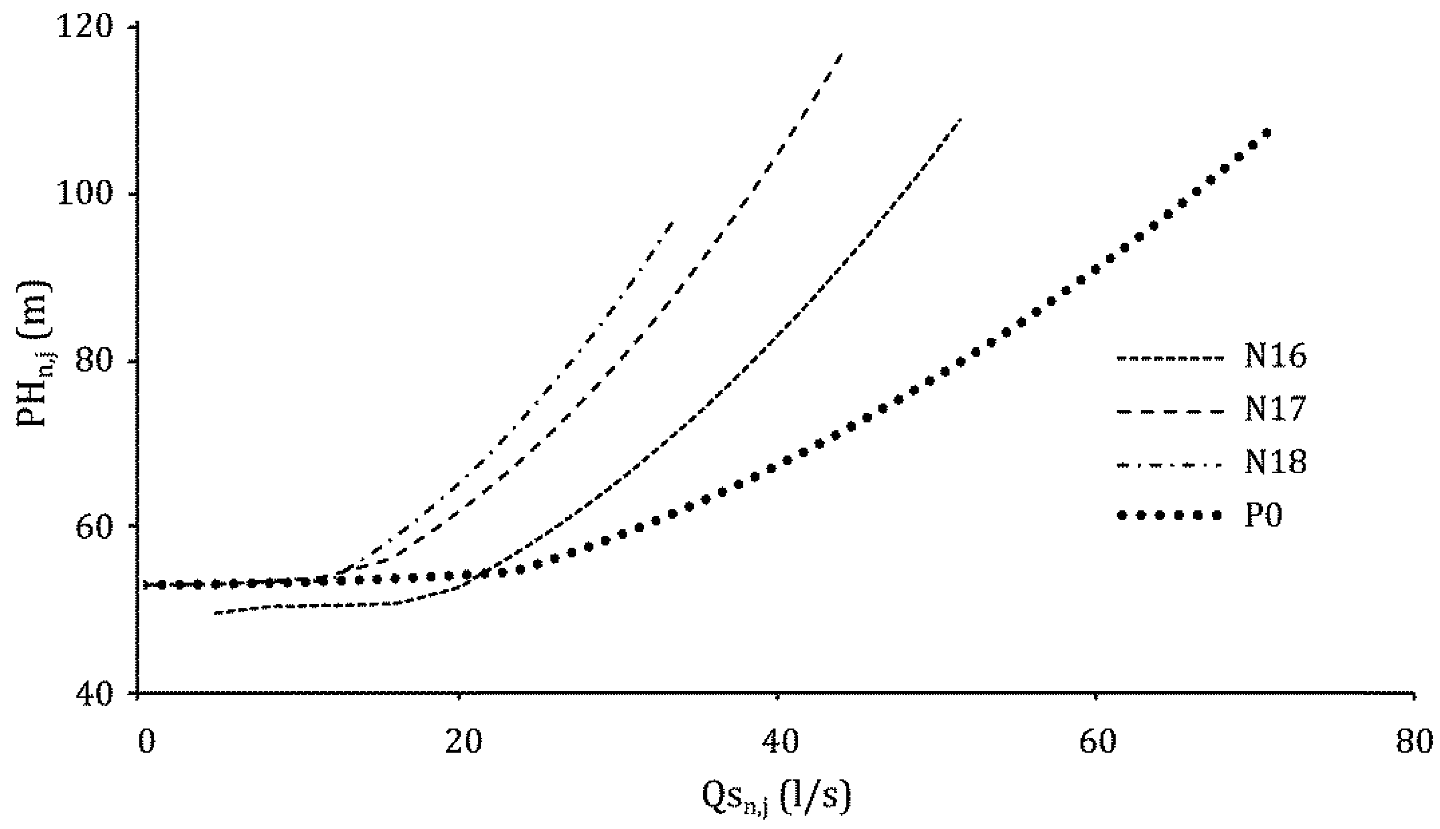
4.1. The TF Network
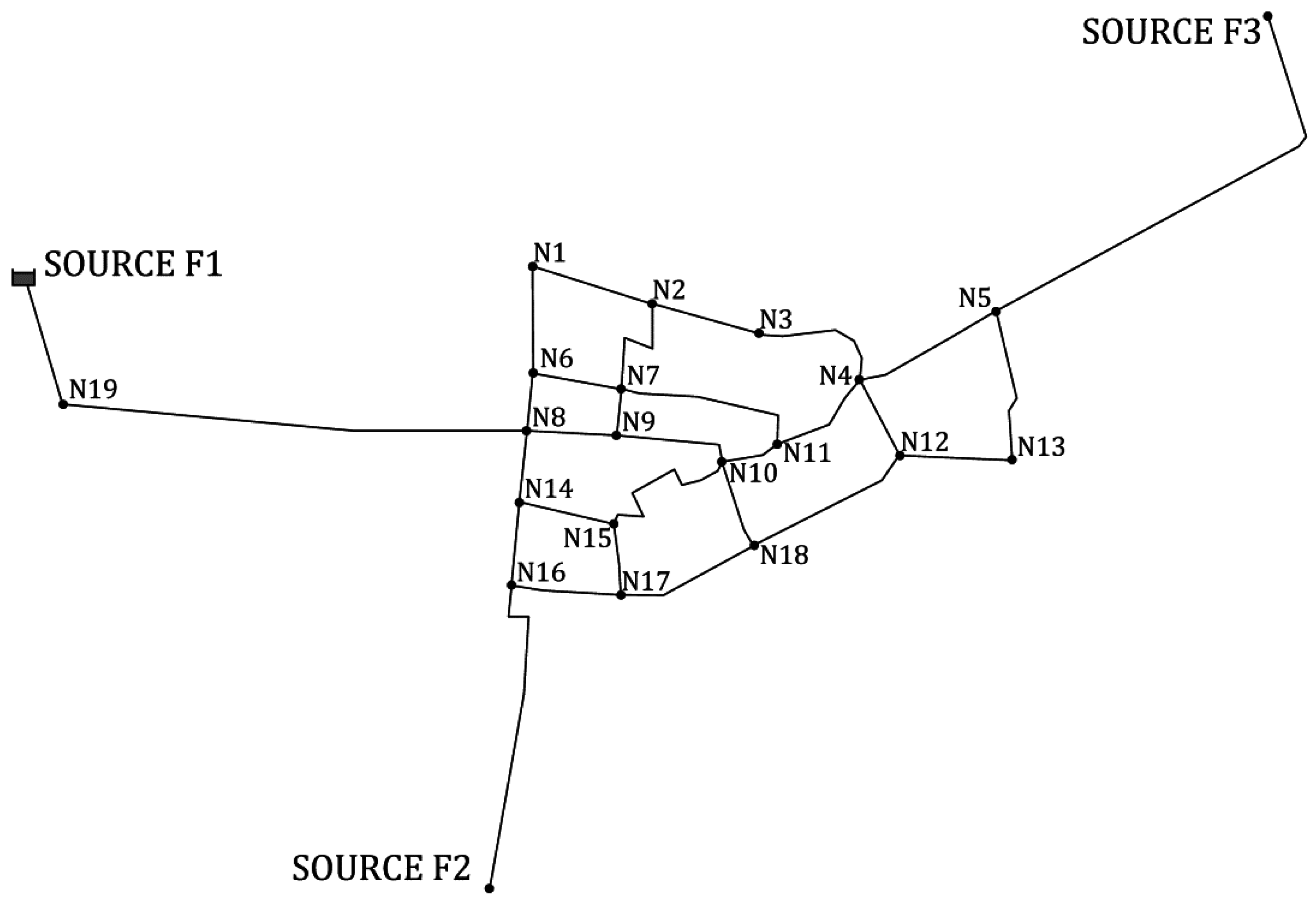
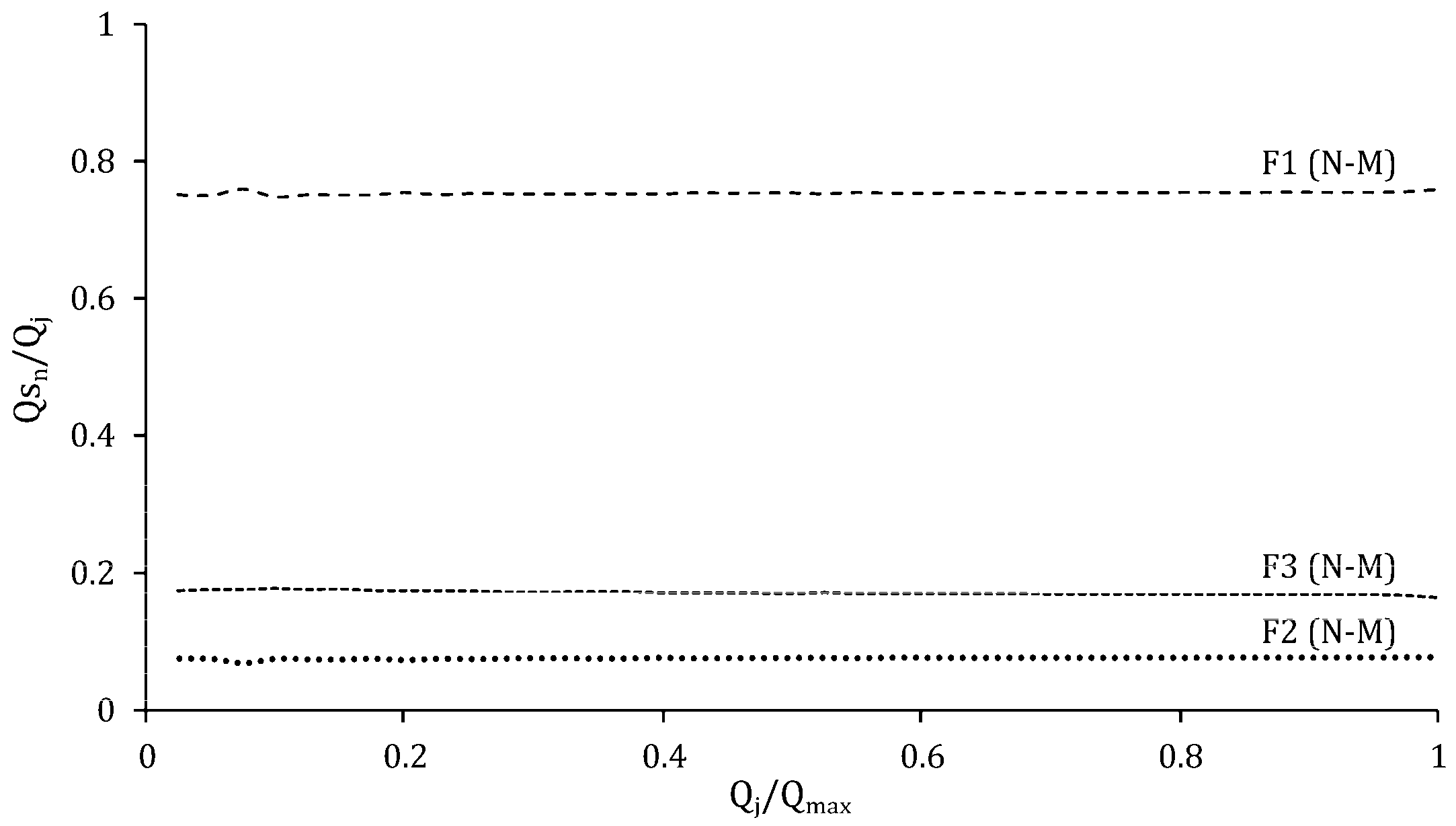
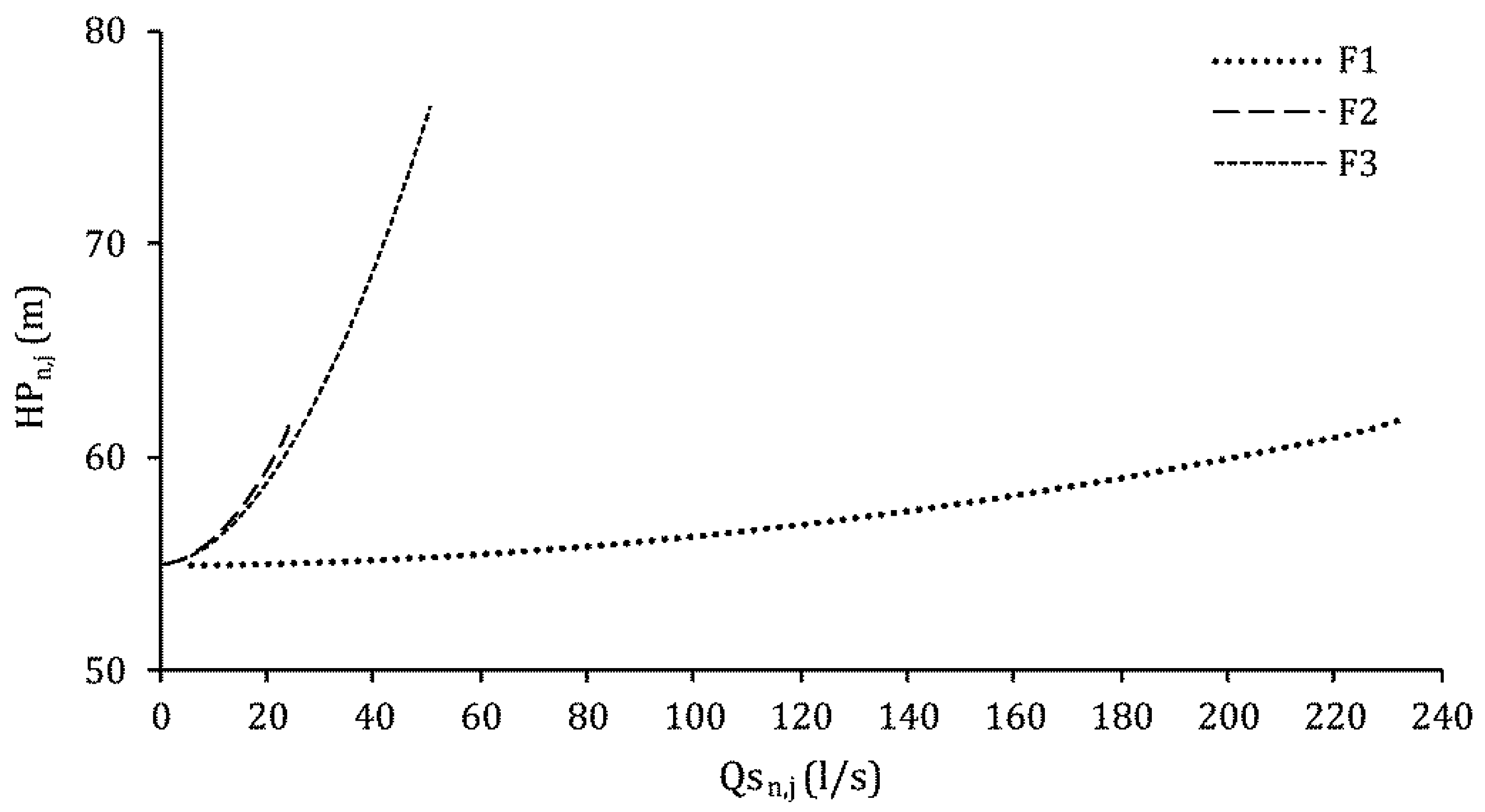
4.2. Catinen Network
5. Conclusions
Acknowledgments
Author Contributions
Conflicts of Interest
References
- Endo, A.; Burnett, K.; Orencio, P.M.; Kumazawa, T.; Wada, C.A.; Ishii, A.; Tsurita, I.; Taniguchi, M. Methods of the water-energy-food nexus. Water 2015, 7, 5806–5830. [Google Scholar] [CrossRef]
- Wu, W.; Gao, J. Enhancing the Reliability and Security of Urban Water Infrastructures through Intelligent Monitoring, Assessment, and Optimization. In Intelligent Infrastructures; Springer: New York, NY, USA, 2010; pp. 487–516. [Google Scholar]
- Yannopoulos, S.I.; Lyberatos, G.; Theodossiou, N.; Li, W.; Valipour, M.; Tamburrino, A.; Angelakis, A.N. Evolution of Water Lifting Devices (Pumps) over the Centuries Worldwide. Water 2015, 7, 5031–5060. [Google Scholar] [CrossRef]
- Frenning, L. Pump Life Cycle Costs: A Guide to LCC Analysis for Pumping Systems. U.S. Department of Energy’s Office of Industrial Technologies, 2001. Available online: http://energy.gov/sites/prod/files/2014/05/f16/pumplcc_1001.pdf (accessed on 27 October 2016). [Google Scholar]
- Perez, R.; Stark, W. The most important pump calculation. Pumps Syst. 2007, May, 24–26. [Google Scholar]
- Graham, S. Low life-cycle cost centrifugal pumps for utility applications. World Pumps 2007, 2007, 30–33. [Google Scholar] [CrossRef]
- Tolvanen, H.J. Life cycle energy cost savings and pump selection. World Pumps 2007, 2007, 34–37. [Google Scholar] [CrossRef]
- Marchi, A.; Salomons, E.; Ostfeld, A.; Kapelan, Z.; Simpson, A.R.; Zecchin, A.C.; Maier, H.R.; Wu, Z.Y.; Elsayed, S.M.; Song, Y.; et al. Battle of the Water Networks II. J. Water Resour. Plan. Manag. 2013, 140. [Google Scholar] [CrossRef]
- Giustolisi, O.; Berardi, L.; Laucelli, D.; Savic, D.; Kapelan, Z. Operational and Tactical Management of Water and Energy Resources in Pressurized Systems: The competition at WDSA 2014. J. Water Resour. Plan. Manag. 2015, 142, C4015002. [Google Scholar] [CrossRef]
- Vitasovic, Z.Z. An Integrated Control Strategy for the Activated Sludge Process. Ph.D. Thesis, Rice University, Houston, TX, USA, 1986. [Google Scholar]
- Yin, M.; Andrews, J.; Stenstrom, M. Optimum Simulation and Control of Fixed-Speed Pumping Stations. J. Environ. Eng. 1996, 122, 205–211. [Google Scholar] [CrossRef]
- Lingireddy, S.; Wood, D.J. Improved Operation of Water Distribution Systems Using Variable-Seed Pumps. J. Energy Eng. 1998, 124, 90–103. [Google Scholar] [CrossRef]
- Planells Alandi, P.; Carrión Pérez, P.; Ortega Álvarez, J.F.; Moreno Hidalgo, M.Á.; Tarjuelo Martín-benito, J.M. Pumping Selection and Regulation for Water-Distribution Networks. J. Irrig. Drain Eng. 2005, 131, 273–281. [Google Scholar] [CrossRef]
- Planells Alandi, P.; Tarjuelo Martín-Benito, J.; Ortega Alvarez, J.; Casanova Martínez, M. Design of water distribution networks for on-demand irrigation. Irrig. Sci. 2001, 20, 189–201. [Google Scholar] [CrossRef]
- Lamaddalena, N.; Khila, S. Efficiency-driven pumping station regulation in on-demand irrigation systems. Irrig. Sci. 2013, 31, 395–410. [Google Scholar] [CrossRef]
- Viholainen, J.; Tamminen, J.; Ahonen, T.; Ahola, J.; Vakkilainen, E.; Soukka, R. Energy-efficient control strategy for variable speed-driven parallel pumping systems. Energy Effic. 2013, 6, 495–509. [Google Scholar] [CrossRef]
- Diaz, J.A.R.; Montesinos, P.; Poyato, E.C. Detecting Critical Points in On-Demand Irrigation Pressurized Networks—A New Methodology. Water Resour. Manag. 2012, 26, 1693–1713. [Google Scholar] [CrossRef]
- Moreno, M.A.; Ortega, J.F.; Córcoles, J.I.; Martínez, A.; Tarjuelo, J.M. Energy analysis of irrigation delivery systems: Monitoring and evaluation of proposed measures for improving energy efficiency. Irrig. Sci. 2010, 28, 445–460. [Google Scholar] [CrossRef]
- Fernández García, I.; Montesinos, P.; Camacho Poyato, E.; Rodríguez Díaz, J.A. Energy cost optimization in pressurized irrigation networks. Irrig. Sci. 2016, 34, 1–13. [Google Scholar] [CrossRef]
- Carrillo Cobo, M.T.; Rodríguez Díaz, J.A.; Montesinos, P.; López Luque, R.; Camacho Poyato, E. Low energy consumption seasonal calendar for sectoring operation in pressurized irrigation networks. Irrig. Sci. 2011, 29, 157–169. [Google Scholar] [CrossRef]
- Fernández García, I.; Rodríguez Díaz, J.A.; Camacho Poyato, E.; Montesinos, P. Optimal Operation of Pressurized Irrigation Networks with Several Supply Sources. Water Resour. Manag. 2013, 27, 2855–2869. [Google Scholar] [CrossRef]
- Fernández García, I.; Montesinos, P.; Camacho, E.; Rodríguez Díaz, J.A. Methodology for Detecting Critical Points in Pressurized Irrigation Networks with Multiple Water Supply Points. Water Resour. Manag. 2014, 28, 1095–1109. [Google Scholar] [CrossRef]
- Araujo, L.S.; Ramos, H.; Coelho, S.T. Pressure Control for Leakage Minimisation in Water Distribution Systems Management. Water Resour. Manag. 2006, 20, 133–149. [Google Scholar] [CrossRef]
- Nazif, S.; Karamouz, M.; Tabesh, M.; Moridi, A. Pressure Management Model for Urban Water Distribution Networks. Water Resour. Manag. 2009, 24, 437–458. [Google Scholar] [CrossRef]
- Pasha, M.F.K.; Lansey, K. Strategies to develop warm solutions for real-time pump scheduling for water distribution systems. Water Resour. Manag. 2014, 28, 3975–3987. [Google Scholar] [CrossRef]
- Giacomello, C.; Kapelan, Z.; Nicolini, M. Fast Hybrid Optimisation Method for Effective Pump Scheduling. J. Water Resour. Plan. Manag. 2013, 193, 175–183. [Google Scholar] [CrossRef]
- Jung, D.; Kang, D.; Kang, M.; Kim, B. Real-time pump scheduling for water transmission systems: Case study. KSCE J. Civ. Eng. 2015, 19, 1987–1993. [Google Scholar] [CrossRef]
- Martínez-Solano, F.J.; Iglesias-Rey, P.L.; Mora-Meliá, D.; Fuertes-Miquel, V.S. Using the Set Point Concept to Allow Water Distribution System Skeletonization Preserving Water Quality Constraints. Procedia Eng. 2014, 89, 213–219. [Google Scholar] [CrossRef]
- Iglesias-Rey, P.L.; Martinez-Solano, F.J.; Mora-Melia, D.; Ribelles-Aguilar, J.V. The battle water networks II: Combination of Meta-Heuristc Technics with the Concept of Setpoint Function in Water Network Optimization Algorithms. In Proceedings of the WDSA 2012: 14th Water Distribution Systems Analysis Conference, Adelaide, Australia, 24–27 September 2012.
- Rossman, L.A. EPANET User Manual; United States Evironmental Protection Agency: Cincinnati, OH, USA, 2000. [Google Scholar]
- Ostfeld, A.; Tubaltzev, A. Ant colony optimization for least-cost design and operation of pumping water distribution systems. J. Water Resour. Plan. Manag. 2008, 134, 107–118. [Google Scholar] [CrossRef]
- López-Ibáñez, M. Operational Optimisation of Water Distribution Networks. Ph.D. Thesis, Edinburgh Napier University, Edinburgh, UK, 2009. [Google Scholar]
- Mora-Melia, D.; Iglesias-Rey, P.L.; Martinez-Solano, F.J.; Fuertes-Miquel, V.S. Design of Water Distribution Networks using a Pseudo-Genetic Algorithm and Sensitivity of Genetic Operators. Water Resour. Manag. 2013, 27, 4149–4162. [Google Scholar] [CrossRef]
- Hooke, R.; Jeeves, T.A. Direct search solution of numerical and statical problems. J. ACM 1961, 8, 212–229. [Google Scholar] [CrossRef]
- Nelder, J.A.; Mead, R. A Simplex Method for Function Minimization. Comput. J. 1965, 7, 308–313. [Google Scholar] [CrossRef]
- Cesario, L. Modeling, Analysis, and Design of Water Distribution Systems; American Water Works Association: St. Louis, MO, USA, 1995. [Google Scholar]
- Martínez-Solano, J.; Iglesias-Rey, P.L.; Pérez-García, R.; López-Jiménez, P.A. Hydraulic Analysis of Peak Demand in Looped Water Distribution Networks. J. Water Resour. Plan. Manag. 2008, 134, 504–510. [Google Scholar] [CrossRef]
- Mora-Melia, D.; Iglesias-Rey, P.L.; Martinez-Solano, F.J.; Ballesteros-Pérez, P. Efficiency of Evolutionary Algorithms in Water Network Pipe Sizing. Water Resour. Manag. 2015, 29, 4817–4831. [Google Scholar] [CrossRef]


| ID | Elev (m) | Demand (L/s) | ID | Elev (m) | Demand (L/s) |
|---|---|---|---|---|---|
| N1 | 8 | 5 | N11 | 7 | 10 |
| N2 | 8 | 4 | N12 | 5 | 5 |
| N3 | 5 | 3 | N13 | 4 | 2 |
| N4 | 8 | 4 | N14 | 3 | 10 |
| N5 | 4 | 3 | N15 | 3 | 15 |
| N6 | 2 | 8 | N16 | 4 | 0 |
| N7 | 5 | 7 | N17 | 0 | 0 |
| N8 | 6 | 10 | N18 | 0 | 0 |
| N9 | 2 | 9 | P0 | 0 | 0 |
| N10 | 7 | 5 |
| Node1 | Node2 | Length (m) | Diameter (mm) | Node1 | Node2 | Length (m) | Diameter (mm) |
|---|---|---|---|---|---|---|---|
| N1 | N2 | 200 | 150 | N11 | N4 | 250 | 150 |
| N2 | N3 | 150 | 100 | N8 | N12 | 250 | 80 |
| N3 | N4 | 150 | 100 | N5 | N13 | 100 | 60 |
| N4 | N1 | 200 | 200 | N3 | N12 | 98 | 60 |
| N5 | N6 | 200 | 60 | N3 | N14 | 300 | 80 |
| N7 | N8 | 400 | 80 | N14 | N15 | 500 | 80 |
| N6 | N7 | 300 | 60 | N2 | N15 | 400 | 100 |
| N8 | N5 | 300 | 80 | N1 | P0 | 1500 | 250 |
| N8 | N4 | 250 | 150 | N16 | N10 | 125 | 100 |
| N7 | N9 | 300 | 100 | N12 | N13 | 52 | 60 |
| N10 | N11 | 300 | 100 | N17 | N12 | 1 | 2000 |
| N9 | N16 | 125 | 100 | N14 | N18 | 1 | 1000 |
| N11 | N7 | 300 | 80 |
| ID | Elev (m) | Demand (L/s) | ID | Elev (m) | Demand (L/s) |
|---|---|---|---|---|---|
| N1 | 9 | 11.9 | N12 | 7.5 | 9.4 |
| N2 | 7 | 7.4 | N13 | 8.5 | 9.6 |
| N3 | 5 | 10.3 | N14 | 9.6 | 8.8 |
| N4 | 7.5 | 4.6 | N15 | 7.8 | 5.3 |
| N5 | 10 | 17.5 | N16 | 10 | 13.8 |
| N6 | 9.6 | 5.1 | N17 | 7.8 | 4.3 |
| N7 | 8 | 4.9 | N18 | 6 | 8.4 |
| N8 | 9.9 | 11 | N19 | 6 | 4.4 |
| N9 | 7.8 | 3.7 | F3 | 0 | 0 |
| N10 | 6 | 7.5 | F2 | 0 | 0 |
| N11 | 5.3 | 6.3 | F1 | 0 | 0 |
| Node1 | Node2 | Length (m) | Diam. (mm) | Roug. | Node1 | Node2 | Length (m) | Diam. (mm) | Roug. |
|---|---|---|---|---|---|---|---|---|---|
| N1 | N6 | 253.26 | 199.20 | 0.03 | N12 | N13 | 268.10 | 148.40 | 0.03 |
| N2 | N1 | 301.88 | 148.40 | 0.03 | N12 | N4 | 191.92 | 199.20 | 0.03 |
| N2 | N3 | 260.79 | 199.20 | 0.03 | N5 | N13 | 391.53 | 123.00 | 0.03 |
| N3 | N4 | 345.08 | 123.00 | 0.03 | N4 | N11 | 268.24 | 148.40 | 0.03 |
| N4 | N5 | 342.25 | 148.40 | 0.03 | N8 | N14 | 169.26 | 250.00 | 0.10 |
| N6 | N7 | 211.13 | 148.40 | 0.03 | N14 | N15 | 239.94 | 250.00 | 0.10 |
| N7 | N2 | 301.81 | 199.20 | 0.03 | N15 | N10 | 384.76 | 123.00 | 0.03 |
| N7 | N9 | 113.47 | 199.20 | 0.03 | N15 | N17 | 165.81 | 148.40 | 0.03 |
| N9 | N8 | 215.97 | 250.00 | 0.10 | N17 | N16 | 261.97 | 199.20 | 0.03 |
| N8 | N6 | 146.87 | 199.20 | 0.03 | N17 | N18 | 354.56 | 148.40 | 0.03 |
| N7 | N11 | 459.60 | 199.20 | 0.03 | N19 | N8 | 1047.55 | 498.00 | 0.03 |
| N11 | N10 | 142.14 | 150.00 | 0.10 | N14 | N16 | 204.87 | 199.20 | 0.03 |
| N10 | N9 | 306.66 | 199.20 | 0.03 | F1 | N19 | 150.00 | 498.00 | 0.10 |
| N10 | N18 | 222.95 | 148.40 | 0.03 | N5 | F3 | 2000.00 | 199.20 | 0.03 |
| N18 | N12 | 438.65 | 148.40 | 0.03 | N16 | F2 | 1300.00 | 199.20 | 0.03 |
© 2016 by the authors; licensee MDPI, Basel, Switzerland. This article is an open access article distributed under the terms and conditions of the Creative Commons Attribution (CC-BY) license (http://creativecommons.org/licenses/by/4.0/).
Share and Cite
León-Celi, C.; Iglesias-Rey, P.L.; Martínez-Solano, F.J.; Mora-Melia, D. A Methodology for the Optimization of Flow Rate Injection to Looped Water Distribution Networks through Multiple Pumping Stations. Water 2016, 8, 575. https://doi.org/10.3390/w8120575
León-Celi C, Iglesias-Rey PL, Martínez-Solano FJ, Mora-Melia D. A Methodology for the Optimization of Flow Rate Injection to Looped Water Distribution Networks through Multiple Pumping Stations. Water. 2016; 8(12):575. https://doi.org/10.3390/w8120575
Chicago/Turabian StyleLeón-Celi, Christian, Pedro L. Iglesias-Rey, F. Javier Martínez-Solano, and Daniel Mora-Melia. 2016. "A Methodology for the Optimization of Flow Rate Injection to Looped Water Distribution Networks through Multiple Pumping Stations" Water 8, no. 12: 575. https://doi.org/10.3390/w8120575