Experimental and Numerical Analysis of Egg-Shaped Sewer Pipes Flow Performance

Abstract

A Computational Fluid Dynamics (CFD) model was developed to analyze the open-channel flow in a new set of egg-shaped pipes for small combined sewer systems. The egg-shaped cross-section was selected after studying several geometries under different flow conditions. Once the egg-shaped cross-section was defined, a real-scale physical model was built and a series of partial-full flow experiments were performed in order to validate the numerical simulations. Furthermore, the numerical velocity distributions were compared with an experimental formulation for analytic geometries, with comparison results indicating a satisfactory concordance. After the hydraulic performance of the egg-shaped pipe was analyzed, the numerical model was used to compare the average velocity and shear stress against an equivalent area circular pipe under low flow conditions. The proposed egg shape showed a better flow performance up to a filling ratio of h/H = 0.25.

1. Introduction

Egg-shaped pipes appear as a suitable geometry for combined sewer sewage networks. Egg-shaped conduits present higher resistance against traffic loads than conventional circular pipes. In addition, this kind of pipe also shows a better hydraulic performance in normal operation dry weather conditions of combined sewer systems, in which a high percentage of the time the flow discharge is conveyed by the lower part of the section. In these conditions, egg-shaped pipes present higher flow velocities due to their smaller wetted perimeter, reducing the sedimentation of particles and the sewer cleaning operational costs [1]. The resuspension of sewer sediments during wet weather flows is an important source of the pollution of Combined Sewer Overflows [2], and their control is one of the main objectives of the integrated urban water management in urban systems [3].

In spite of the structural and hydraulic advantages, egg-shaped pipes are not commonly used in the construction of small combined sewer systems because of their highest production costs. Nevertheless, with the evolution of production techniques such as plastic injection or extrusion, the fabrication costs of plastic egg-shaped pipes can be as competitive as circular plastic pipes. In this work we present the first stage of the collaborative OvalPipe R&D project that aims to develop a new functioning egg-shaped plastic pipe that is commercially viable and market competitive with the 300–400 mm diameter circular pipes.

The first steps of the process consisted in the geometric definition and in the hydraulic analysis of the egg-shaped cross section. The egg-shaped geometry was designed with the objective of maximizing the hydraulic radius under low flow conditions and the discharge capacity under full-depth or near full-depth conditions. Once the cross-section was defined, a real-scale egg-shaped pipe was built at a laboratory facility to study its hydraulic characteristics.

Most of the open-channel pipe flow studies were performed in circular conduits. For instance, the early studies of turbulence developed by Nezu and Nakagawa [4] proposed different formulations to describe velocity profiles in circular cross-sections. Guo et al. [5] developed new velocity distribution formulas for circular, elliptic, parabolic, and hyperbolic open-channels (hereinafter named as conic open-channels). Particle Image Velocimetry (PIV) technique was also developed to determine velocity distribution in small circular pipes [6]. Nevertheless, detailed hydrodynamic experiments for egg-shaped pipes are missing.

In order to analyze the behavior of the circular and egg-shaped pipes, open-channel flow experiments were conducted with ANSYS CFX Computational Fluid Dynamics (CFD) code. To simulate the open-channel flow in closed conduits such as pipes, a two-phase flow model was developed to solve the interactions between liquid (water) and gas (air) interface [7,8,9,10]. The experimental velocity profiles and shear stress values were compared with the numerical results, following the methodology proposed in previous studies [11]. Finally, numerical results from egg-shaped and circular pipe analysis were also compared with the analytical open-channel flow Manning and Thormann-Franke equations.

2. Materials and Methods

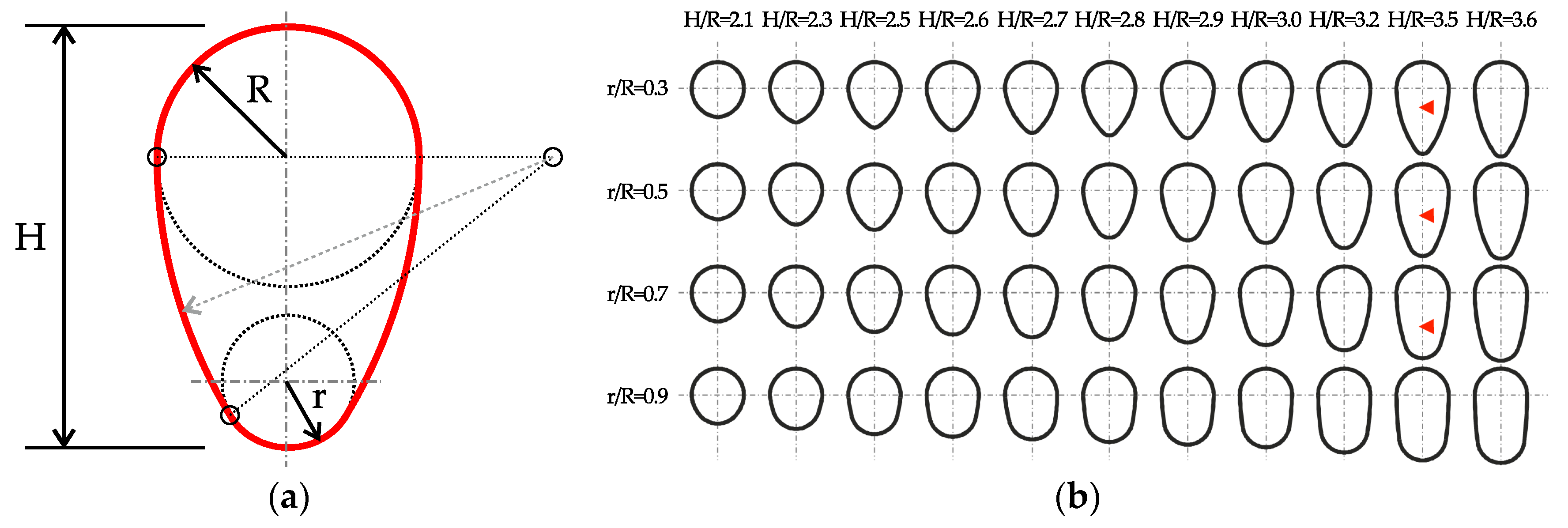
2.1. Egg-Shaped Section Definition

In the first step of the study an egg-shaped cross section was defined with an equivalent area to a 315 mm circular pipe (300 mm inner diameter). In terms of geometric construction of the egg-shaped profile, it was possible to use different families of curves and ellipses, sinusoidal functions, arcs, or specific methods. In the present work, a combination of arcs was chosen in order to build an egg-shaped cross-section (Figure 1a). This cross-section was defined from three variables: the top and bottom radii (R and r) and the total height (H). In order to define the transition curve between the upper and bottom circumferences, the construction method proposed by other authors was allowed, where the circular lateral arcs have their centers at the same height as the top circumference center [12]. Thus, the r/R and H/R ratios allow the design of a wide variety of theoretical ovoids with different aspect ratios, which potentially could be used in the field of sanitation and urban drainage engineering.

A set of egg-shaped cross-sections with ratios r/R between 0.3 and 0.9 and H/R between 2.1 and 3.6 were compared with a 300 mm inner diameter circular section (Figure 1b). All the proposed theoretical ovoids have the same area as the circular pipe. The performance of the pipes was analyzed by means of the hydraulic radius in low-depth condition and the full filling discharge capacity determined with the Manning’s Equation for uniform flow:

$$U_{av}=R_h^{2/3}\sqrt{S}/n$$

(1)

where U_av is the average velocity (m/s), R_h is the hydraulic radius (m), S is the slope of the pipe (m/m) and n is the Manning’s roughness coefficient (s/m^1/3). According to this equation, a higher hydraulic radius means a higher mean velocity, hydraulic performance, and more sediment transport capacity. The circular geometry shows the highest full-bore discharge capacity as it presents the largest hydraulic radius regarding any cross-section with the same area. Nevertheless, in low flow conditions the egg-shaped conduit has a lower hydraulic radius. Therefore, the best aspect ratio for the egg-shaped cross-section should fit a higher hydraulic radius under low flow conditions but without losing significant full-filling discharge capacity regarding the circular discharge value.

The hydraulic conditions to perform the analysis of the different pipe shapes were a slope S = 0.2% and a Manning’s coefficient n = 0.012 s/m^1/3, resulting in a full-filling discharge capacity of 47 L/s for the 300 mm circular pipe. Dry weather flow conditions were calculated using three different rates of daily average wastewater flow to wet weather flow (1:10, 1:20, and 1:50). Assuming a certain safety margin, the full-bore discharge capacity was set to a value of Q₀ = 40 L/s. The resulting base-flow discharges were 4.0, 2.0, and 0.8 L/s, respectively. From the whole set of the different egg-shaped pipes analyzed, the cross-sections with the highest hydraulic radius for each low flow condition and maximal full-filling discharge are those with H/R = 3.5 and r/R = 0.7, 0.5, and 0.3, respectively (

Table 1. Comparison of hydraulic radius (R_h) for low flows (1:10, 1:20, and 1:50 wastewater and rainfall rates) and full-bore section discharges (Q₀) conditions in egg-shaped cross-sections with best hydraulic performance. Hydraulic radius and discharges were normalized with circular cross-section values.

H/R	r/R	Rh 1:10	Rh 1:20	Rh 1:50	Rh Q0	Q0
3.5	0.3	1.038	1.103	1.193	0.905	0.934
3.5	0.5	1.064	1.125	1.187	0.897	0.930
3.5	0.7	1.078	1.114	1.132	0.925	0.949

). The differences found in the hydraulic performance do not justify the commercial development of three egg-shaped pipe sets, so the cross-section with ratios H/R = 3.5 and r/R = 0.5 was chosen because it presents adequate yields in all conditions. It was found that a typical value of H/R in egg-shaped pipe design is 3.0 [12], but the cross-section with ratio H/R = 3.5 has a similar hydraulic performance and improves its momentum of inertia by 15.3%. Therefore, the egg-shaped section with equivalent target area has a total height of 385 mm, a top radius of 110 mm, and a bottom radius of 55 mm.

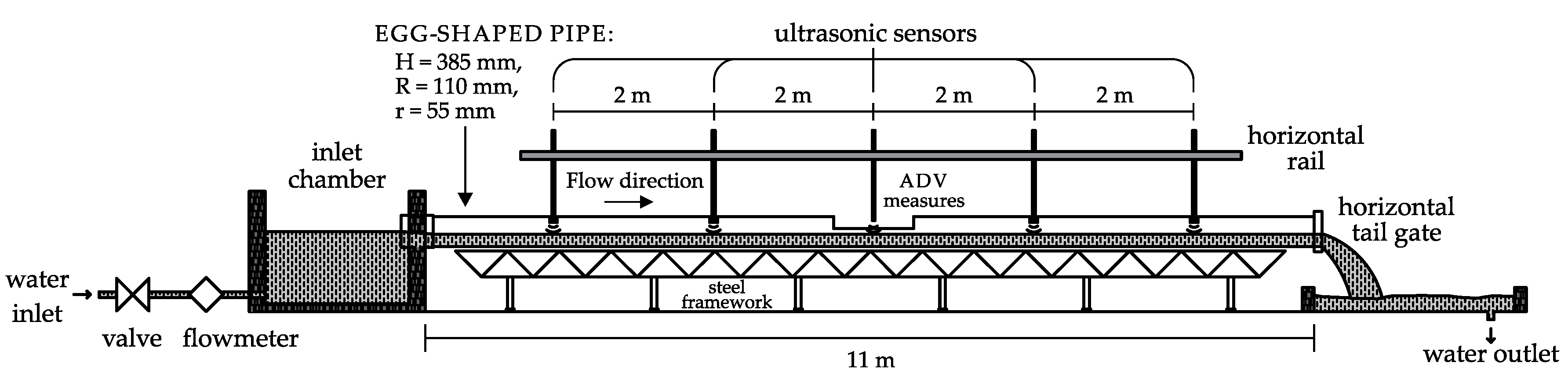
2.2. Experimental Set-Up

A series of experiments were carried out in a physical model of an egg-shaped pipe located at the R&D Centre of Technological Innovation in Building and Civil Engineering (CITEEC) of the University of A Coruña (Figure 2). This model consisted of an 11 m long stainless steel egg-shaped pipe with R = 110 mm, H = 385 mm, and r = 55 mm. At the beginning of the pipe an inlet chamber was placed, while a horizontal tail gate was provided to allow the adjustment of water levels and flow uniformity downstream of the pipe. Water level was measured using five ultrasonic sensors distributed along several apertures opened in the pipe. The resolution of sensors was 0.13 mm and the deviation of ultrasonic beam was 4.6°. Discharge was measured using an ultrasonic flowmeter with an accuracy of ±1% of measured values and registered with a data logger during each test.

Four experiments were conducted at a 0.2% slope with different filling ratios (h/H) of 0.2 to 0.5. Uniform flow conditions were established by adjusting the position and height of a downstream tailgate. Centerline velocity profiles were measured with a Nortek Vectrino© (Rud, Norway) Acoustic Doppler Velocimeter (ADV) with an accuracy of ±1 mm/s at a distance of 5.5 m from the inlet chamber. Water velocity was measured with a spatial resolution of 5 and 2.5 mm for measures close to the pipe bottom and with a sampling frequency of 25 Hz during 300 s to ensure that the measured streamwise turbulence intensity was within 5% of its measured long-term average. All velocity data were de-spiked using the phase-space thresholding method [13,14].

2.3. CFD Model

Numerical simulations were performed with ANSYS CFX software (Canonsburg, PA, USA). This code solves the 3D Reynolds-Averaged Navier-Stokes (RANS) equations [15]. A two-phase flow model was selected to simulate the interaction of the air friction with the water surface in partially filled pipes (Thormann-Franke formulation). In order to calculate the interface between both fluids, ANSYS CFX uses the volume of fluid (VOF) model. In the VOF model, multi-phase fluids share governing equations of mass and momentum conservation. The VOF model tracks the interface position between phases at control volumes within the domain. For this, volume fractions are assigned to each control volume [9].

An unstructured (block-structured) non-uniform mesh was selected to discretize pipe geometry. To avoid convergence problems at the interface between fluids (air-water), the height of the mesh elements was reduced progressively from 3 mm in the main fluid body to 1 mm close to the pipe wall and to the interface [16,17]. As the position of the interface varied in each case because of the water level, a new grid system was necessary for each simulation. The average mesh size in the whole pipe was ~3 × 10⁶ hexahedral elements.

Boundary conditions were set from experimental flow conditions. At the inlet of the channel, discharge and water level were established to constant values depending on the position of each phase. At the outlet, the water level was also fixed. The initial condition imposed to the model was the average velocity obtained from the experiments. Additionally, a steady state simulation in combination with the Shear Stress Transport turbulence model was selected for all cases. Wall function was set by the wall roughness that was established with Manning’s coefficient (n = 0.012 s/m^1/3) for the real egg-shaped pipe. However, the roughness in the numerical model is defined as an equivalent roughness (k_s) which can be estimated as a function of n by means of the Strickler’s equation (n = k_s^1/6/25). Applying this equation, the value of equivalent roughness in the numerical model was set to k_s = 0.729 mm.

3. Results

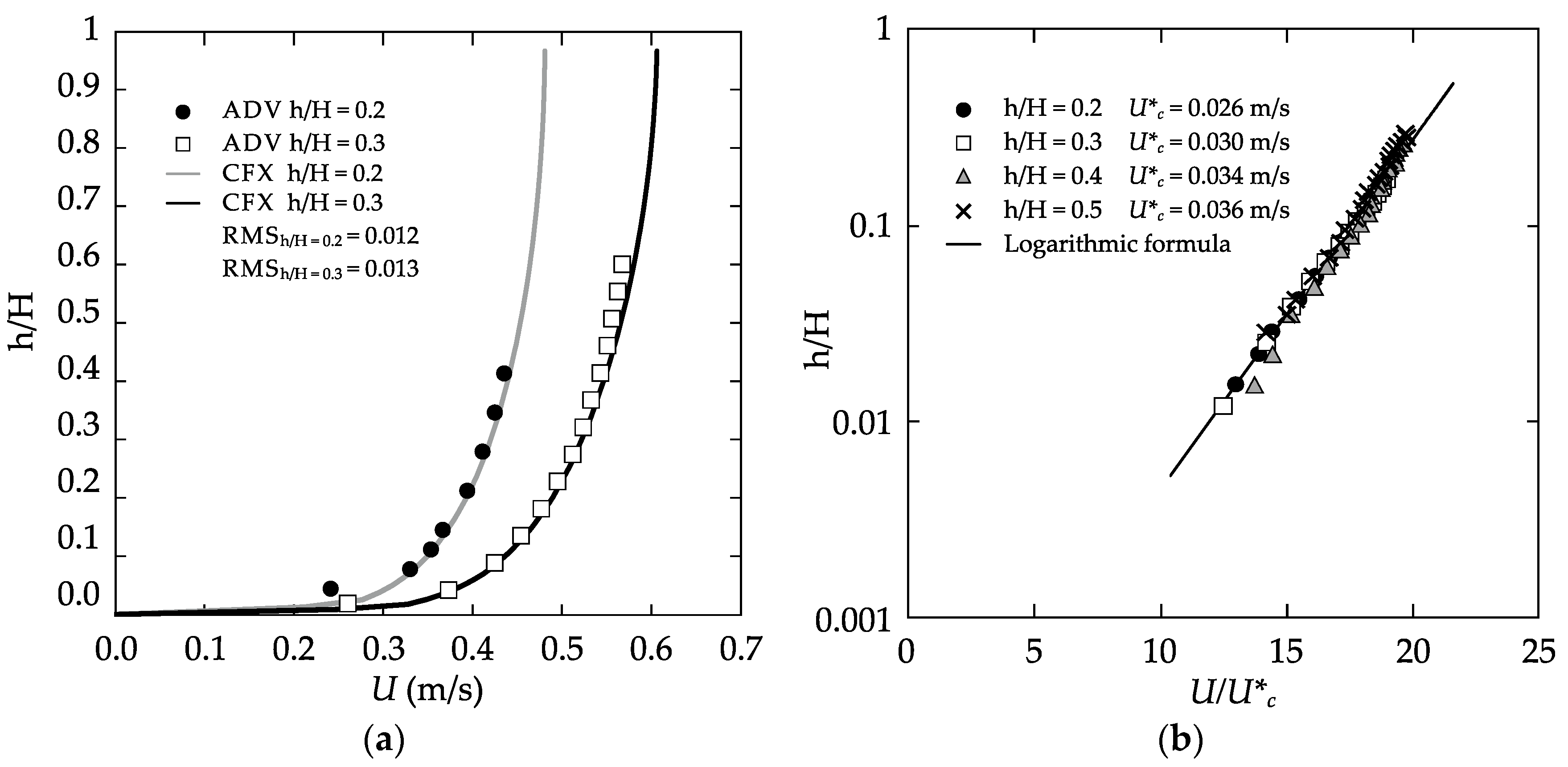
3.1. Boundary Shear Stress and Centreline Velocity Profiles

The shear stress over the wetted perimeter and the centerline velocity profile were used in order to compare CFD model outputs and the flume tests measurements. Discharges ranging from 3.20 to 19.03 L/s were used, resulting in different uniform conditions of water depth and Reynolds number variations. From the experimental data, total shear stress can be expressed as a function of the average friction velocity U_*av with the equation τ = ρU_*av², where ρ is the fluid density (kg/m³). The average friction velocity was calculated as U_*av = (gR_hS)^1/2, with S the slope of the pipe (%), R_h the hydraulic radius (m), and g the gravity acceleration (m/s²). The differences between experimental and output modelling shear stress were less than 10% (

Table 2. Experimental parameters: discharge Q (L/s), averaged velocity U_av (m/s), filling ratio h/H (dimensionless), hydraulic radius R_h (m), Reynolds number Re, average friction velocity U_*av (m/s). Total shear stress results from the experimental methodology τ and output modelling shear stress τ_CFD (N/m²) (relative errors are in parenthesis).

Test	Experimental Conditions						CFD Model
	Q (L/s)	Uav (m/s)	h/H (-)	Rh (m)	Re (×103)	τ = ρU*av2 (N/m2)	τCFD (N/m2)
1	3.20	0.410	0.2	0.034	5.7	0.684	0.664	(−2.9%)
2	7.04	0.528	0.3	0.045	9.5	0.883	0.964	(9.2%)
3	13.08	0.582	0.4	0.057	13.3	1.121	1.159	(3.4%)
4	19.03	0.658	0.5	0.064	16.8	1.254	1.374	(9.6%)

).

The CFD model centerline profiles were compared with the ADV measurements at the middle-section of the pipe (Figure 3a). The agreement between experimental and numerical velocity series was estimated with the root mean square (RMS). RMS < 0.076 was found to be an acceptable fit for all the cases. In addition, vertical velocity profiles can be used to obtain centerline shear stress as an estimation of the friction in the pipe bottom. In open-channel flows, this value is related with the logarithm region of the vertical velocity profile (0.05–0.2 h/H) following a log-law approach [4]:

$$\frac{U(z)}{U_{*c}}=\frac{1}{\mathsf{\kappa }}\ln \left(\frac{z}{k_s}\right)+A_r$$

(2)

where U(z) is the centerline velocity at the height z, U_*c is the centerline friction velocity, κ is the von Kármán constant, k_s is the equivalent roughness (0.729 mm), and A_r is a constant of integration from Prandtl’s mixing-length formulation. In open-channel flows a value of κ = 0.41 is accepted [4]. Both centerline friction velocity and constant of integration were fitted from Equation (2) using a numerical routine, resulting in a value of A_r = 7.9. Figure 3b shows the visual performance of the logarithmic formula and the friction velocity U_*c results. Note that the figure axes are normalized with the total height of the pipe and the value of U_*c for each experiment respectively.

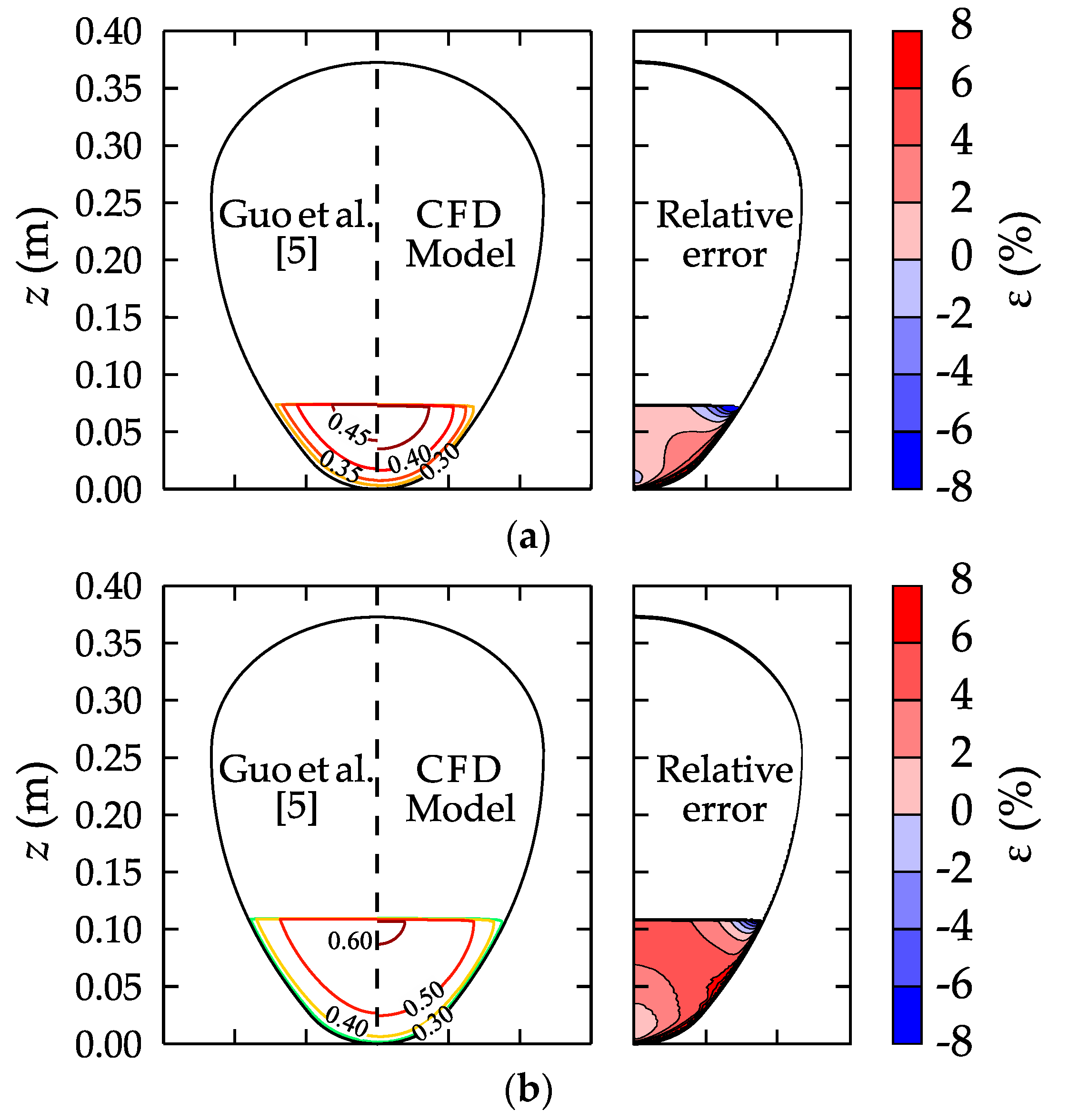
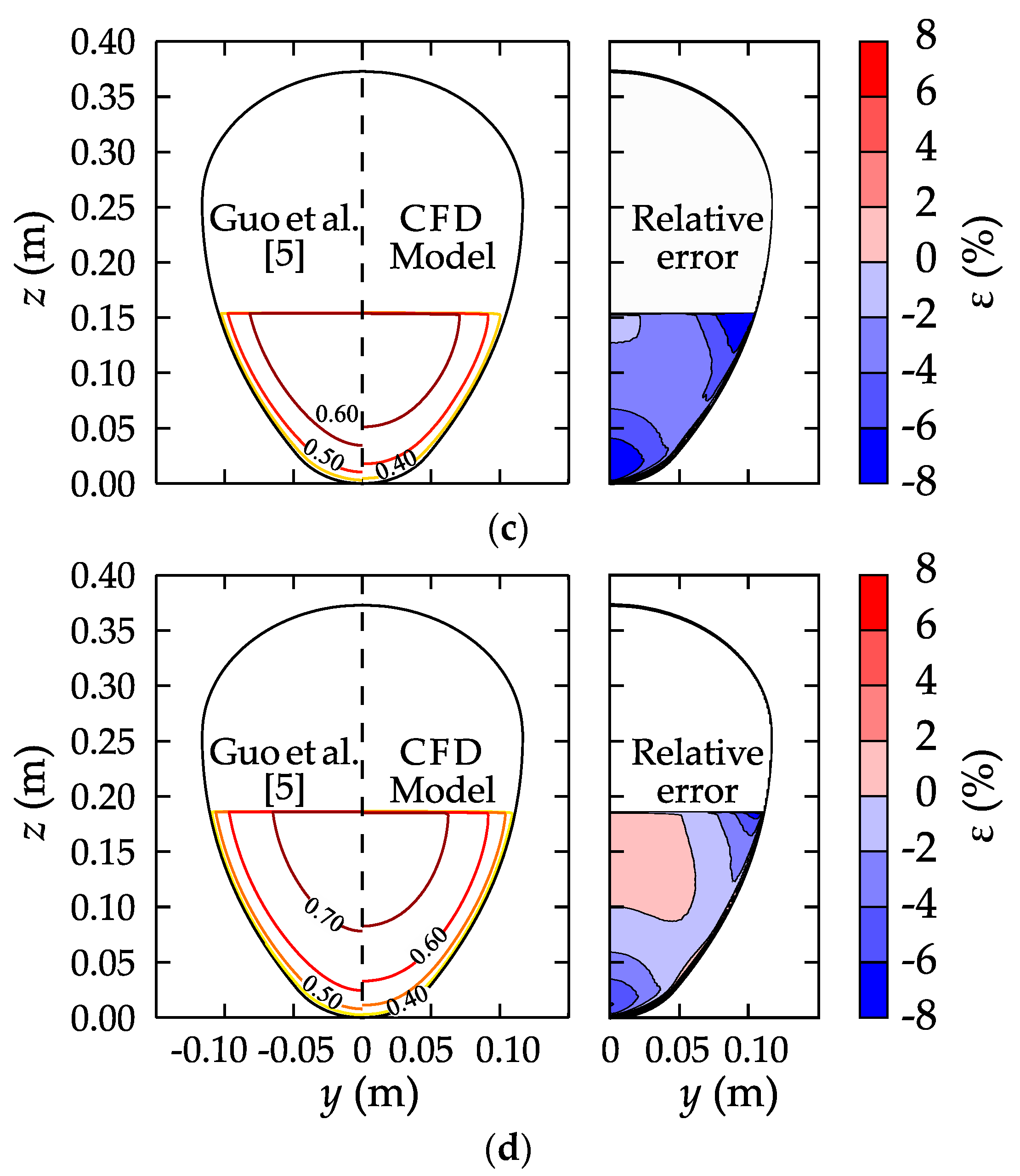
3.2. Cross-Sectional Velocity Distributions

In this section CFD model outputs were compared with the formulation of Guo et al. [5] for the cross-sectional velocity distribution. Guo et al. [5] proposed a simple velocity distribution model for conic open-channels without fitting any parameter. Their experiments were motivated by a design for fish stream-crossing, but they suggested that this model was also valid for self-cleaning drainage systems. The analytical model was tested in a circular metal pipe but no laboratory data of non-circular conic sections were available to validate this formulation. Following the approach by Guo et al. [5], the cross-sectional velocity distribution (U(y,z)) in an egg-shaped or a generic conic geometry can be calculated as a function of the averaged shear velocity U_*av and the centerline shear velocity U_*c (Figure 3b):

$$U(y,z)=\frac{\mathsf{\lambda }{U}_{*av}}{\mathsf{\kappa }}\left[\ln \left(\frac{z}{z_0}\right)-\frac{1}{3}{\left(\frac{z}{\mathsf{\delta }}\right)}^3\right]-U_{*av}\mathsf{\phi }\left(y,y_b\right)$$

(3)

where y and z are the cross-sectional coordinates. In the first term of the Equation (3), λ = U_*c/U_*av is the ratio of the centerline to the average shear velocity (1.02 ± 0.02 range) and z₀ is the hydrodynamic roughness length of the pipe wall. This term approaches the velocity profile at the logarithmic zone, as in Equation (2). Comparing both equations, the value of z₀ can be expressed through the relation A_r = ln(k_s/z₀)/κ, resulting in a value of z₀ = 0.0285 mm. Furthermore, Guo et al. [5] introduced a cubic deduction to the logarithmic equation near the water surface, which depends on the velocity-dip position from the bottom (δ). The velocity-dip position varies depending on the discharge and the secondary currents. This variable was set equal to the surface water level, as no dip-phenomenon was observed either in the numerical or experimental velocity profiles (see Figure 3a). The last term represents the reduction of the velocity distribution because of the cross-section contour, where $\mathsf{\phi }\left(y,y_b\right)$ is the velocity-defect function defined below (y_b represents the pipe’s half-width coordinate):

$$\mathsf{\phi }(y,y_b)=-\frac{1}{\mathsf{\kappa }}\left\{\ln \left(1-\left|\frac{y}{y_b}\right|\right)+\frac{1}{3}\left[1-{\left(1-\left|\frac{y}{y_b}\right|\right)}^3\right]\right\}$$

(4)

All test conditions were reproduced with Guo et al.’s velocity distribution model and they were compared with numerical results, resulting in relative errors under 8% (Figure 4). In order to evaluate the velocity distributions accuracy, the discharges integrated from the approach by Guo et al. [5] were compared with CFD model input values, which were set from experimental measurements. The differences between both discharges were less than 5% (

Table 3. Comparison of CFD/experimental discharges with the values obtained from Guo et al.’s formula [5]. Relative errors are in parenthesis.

Q (L/s)	h/H = 0.2		h/H = 0.3		h/H = 0.4		h/H = 0.5
CFD/Experimental	3.20		7.04		13.08		19.03
Guo et al. [5]	3.06	(−4.4%)	6.72	(−4.5%)	13.51	(3.3%)	19.02	(−0.1%)

).

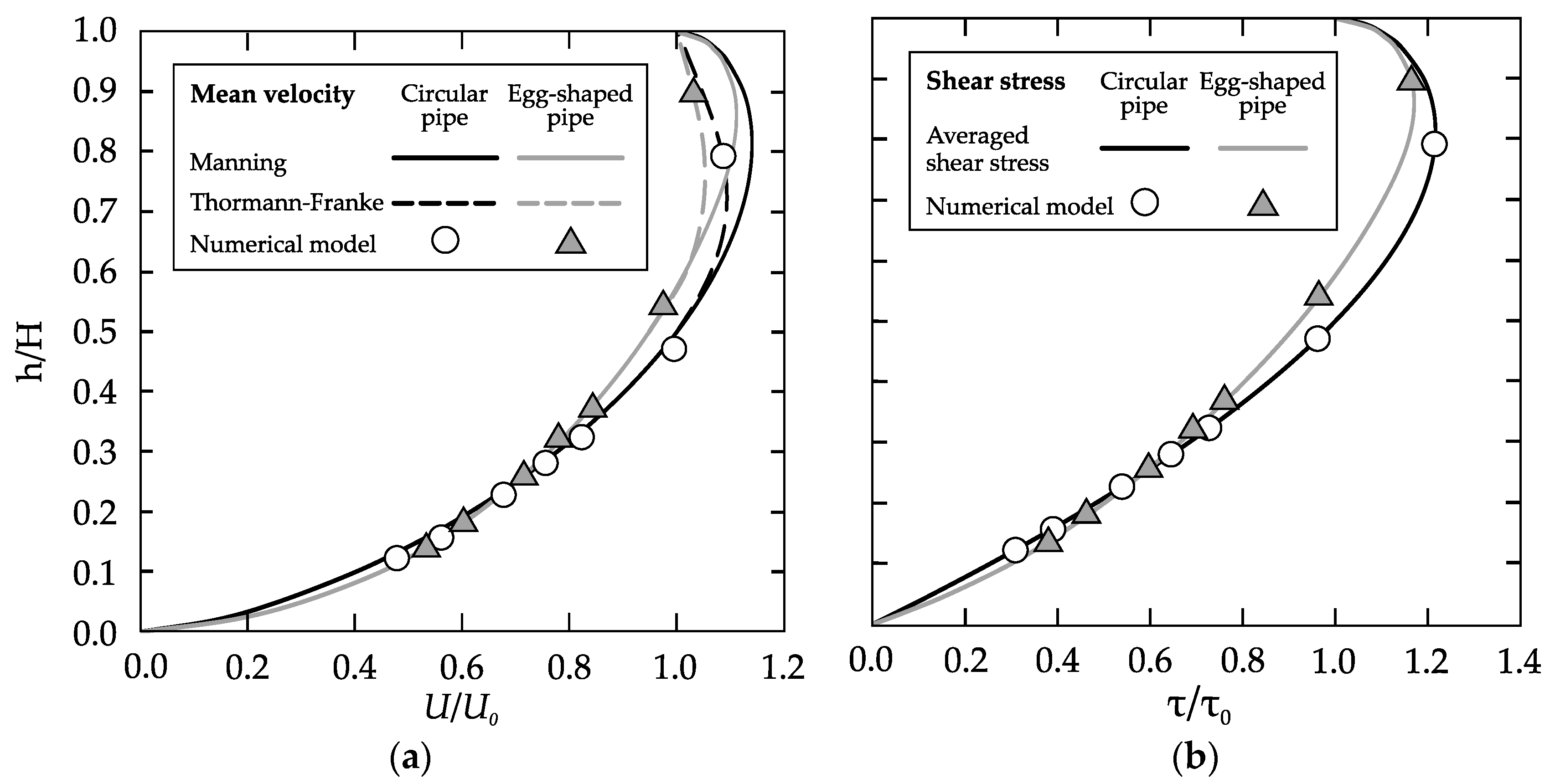
3.3. Numerical Comparison of Circular and Egg-Shaped Mean Flow Behavior

Lastly, the egg-shaped cross-section conduit behavior was compared against a circular section with an equivalent area in order to evaluate its efficiency in partially filled pipe flow. A CFD model was performed for a circular pipe with an inner diameter of 300 mm, which corresponds roughly to a standard 315 mm Polyvinyl Chloride (PVC) sewer pipe. A series of simulations were conducted in both an egg-shaped and circular cross-section model. For each simulation the same hydraulic conditions were used (S = 0.2%, n = 0.012 s/m^1/3). The tested flow discharges were 1.5, 2.5, 5.0, 7.5, 10.0, 20.0, and 40.0 L/s, using more resolution for low-depths ratios. In order to reach uniform flow conditions at the analyzed central section, the upstream and downstream water depths were established with Manning’s Equation.

Flow mean velocity and averaged shear stress results are compared in Figure 5 for circular and egg-shaped pipes. Note that the axes are normalized with the height of each conduit and their full-depth mean velocity (U₀) and shear stress (τ₀) were calculated with Manning’s Equation and averaged shear stress formula (τ = (gR_hS)^1/2), respectively. Egg-shaped cross-section pipe presented higher mean velocity and shear stress values up to a filling ratio of h/H = 0.25, which is over the design cross-section depth for combined sewer pipelines in operating condition (dry weather flow regime). For common operating filling ratios of 0.10 and 0.15, the improvement of the shear stress was 15% and 9%, respectively. Thus, for relative depths h/H < 0.25 a greater sediment transport capacity is expected in the egg-shaped cross-section than in the equivalent-area circular pipes because of the higher velocity and shear stress values. This should reduce the risk of sediment accumulation at the pipe bottom and decrease the risk of pollution associated with sediment deposits [18]. The circular cross-section had a better performance above a filling ratio of h/H = 0.25, which is outside of the range of normal operating conditions of a combined sewer network. For full-filling conditions, the performance of the egg-shaped pipe in terms of averaged shear stress was only a 5.3% lower than the equivalent circular profile.

Numerical results were also compared with the analytical open-channel flow Manning and Thormann-Franke formulas in Figure 5. The Thormann-Franke correction coefficients for egg-shaped sections were obtained in Fresenius et al. [19]. It can be observed that there is a good fit between the numerical and analytical mean velocities and averaged shear stress. Thus, the CFD 3D-RANS model reproduces the Thormann-Franke flow reduction due to air friction in the pipes.

4. Conclusions

Within the framework of an R&D project a new egg-shaped cross-sectional pipe for small combined sewer systems was defined and analyzed. The geometric definition resulted from an analysis of dry-weather flow conditions in sewers. As the main source of pollution in low-flow conditions is the sedimentation at the bottom of pipes, egg-shaped pipes will improve the transport of solids because this section presents a lower hydraulic radius than standard circular pipes during dry weather flow conditions.

To study the hydraulic characteristics of the egg-shaped pipe, a CFD model was developed so that the egg-shaped profile could be compared with an equivalent-area circular section. The CFD model was validated with a set of experiments in an egg-shaped cross-section metal pipe. Velocity profiles and shear stress were used to compare the numerical model and the experimental results, obtaining a good agreement. Furthermore, the numerical velocity distributions were compared with an experimental formulation for analytic geometries resulting in a satisfactory concordance.

Once the hydraulic characteristics of the egg-shaped cross-section were analyzed, a circular pipe with an equivalent area was modeled. Several discharge conditions were simulated mainly for low-depth ratios. At the same time, numerical results were compared with analytical Manning and Thormann-Franke open-channel flow formulas. It was proved that egg-shaped cross-section pipes present better hydraulic characteristics for dry-weather flows up to h/H = 0.25 filling ratio in terms of mean velocities and averaged shear stress values. The results of this study suggest that egg-shaped cross-section pipes may be competitive with conventional circular pipes for the design of combined sewer systems.

References

1. Butler, D.; Davies, J. Urban Drainage, 2nd ed.; CRC Press: Boca Raton, FL, USA, 2004. [Google Scholar]
2. Suarez, J.; Puertas, J. Determination of COD, BOD, and suspended solids loads during combined sewer overflow (CSO) events in some combined catchments in Spain. Ecol. Eng. 2005, 24, 199–217. [Google Scholar] [CrossRef]
3. Suarez, J.; Puertas, J.; Anta, J.; Jacome, A.; Alvarez-Campana, J.M. Gestión integrada de los recursos hídricos en el sistema agua urbana: Desarrollo Urbano Sensible al Agua como enfoque estratégico. Ingeniería Agua 2014, 18, 111–123. [Google Scholar]
4. Nezu, I.; Nakagawa, H. Turbulence in Open-Channel Flows; A.A. Balkema: Rotterdam, The Netherlands, 1993. [Google Scholar]
5. Guo, J.; Mohebbi, A.; Zhai, Y.; Clark, S.P. Turbulent velocity distribution with dip phenomenon in conic open channels. J. Hydraul. Res. 2015, 53, 73–82. [Google Scholar] [CrossRef]
6. Yoon, J.I.; Sung, J.; Ho Lee, M. Velocity profiles and friction coefficients in circular open channels. J. Hydraul. Res. 2012, 50, 304–311. [Google Scholar] [CrossRef]
7. Newton, C.H.; Behnia, M. Numerical calculation of turbulent stratified gas–liquid pipe flows. Int. J. Multiph. Flow 2000, 26, 327–337. [Google Scholar] [CrossRef]
8. Ghorai, S.; Nigam, K.D.P. CFD modeling of flow profiles and interfacial phenomena in two-phase flow pipes. Chem. Eng. Process. 2006, 45, 55–65. [Google Scholar] [CrossRef]
9. De Schepper, S.C.K.; Heynderickx, G.J.; Marin, G.B. CFD modeling of all gas-liquid and vapor-liquid flow regimes predicted by Baker chart. Chem. Eng. J. 2008, 138, 349–357. [Google Scholar] [CrossRef]
10. Bhramara, P.; Rao, V.D.; Sharma, K.V.; Reddy, T.K.K. CFD Analysis of Two Phase Flow in a Horizontal Pipe–Prediction of Pressure Drop. Momentum 2009, 10, 476–482. [Google Scholar]
11. Berlamont, J.E.; Trouw, K.; Luyckx, G. Shear stress distribution in partially filled pipes. J. Hydraul. Eng. 2003, 129, 697–705. [Google Scholar] [CrossRef]
12. Hager, W.H. Wastewater Hydraulics: Theory and Practice; Springer: Berlin, Germany, 2010. [Google Scholar]
13. Goring, D.G.; Nikora, V.I. Despiking Acoustic Doppler Velocimeter Data. J. Hydraul. Eng. 2002, 128, 117–126. [Google Scholar] [CrossRef]
14. Cea, L.; Puertas, J.; Pena, L. Velocity measurements on highly turbulent free surface flow using ADV. Exp. Fluids 2007, 42, 333–348. [Google Scholar] [CrossRef]
15. ANSYS CFX. ANSYS CFX-Solver Theory Guide; ANSYS CFX Release: Canonsburg, PA, USA, 2012; Volume 11, pp. 69–118. [Google Scholar]
16. Lun, I.; Calay, R.K.; Holdo, A.E. Modelling two-phase flows using CFD. Appl. Energy 1996, 53, 299–314. [Google Scholar] [CrossRef]
17. Vallée, C.; Höhne, T.; Prasser, H.M.; Sühnel, T. Experimental investigation and CFD simulation of horizontal stratified two-phase flow phenomena. Nucl. Eng. Des. 2008, 238, 637–646. [Google Scholar]
18. Ashley, R.; Bertrand-Krajewski, J.L.; Hvitved-Jacobsen, T.; Verbanck, M. Solids in Sewers; Scientific & Technical Report 14; IWA Publishing: London, UK, 2004. [Google Scholar]
19. Fresenius, W.; Schneider, W.; Böhnke, B.; Pöppinghaus, K.M. Manual de Disposición de Aguas Residuales: Origen, Descarga, Tratamiento y Análisis de las Aguas Residuales; CEPIS: Lima, Peru, 1991. [Google Scholar]
Figure 1. (a) Egg-shaped cross-section definition from variables H, R, and r with a tangent connecting top and bottom arcs and (b) H/R and r/R relationships. The best egg-shaped cross-sections are highlighted with triangles.
Water 08 00587 g001
Figure 2. Schematic drawing of the physical model.
Water 08 00587 g002
Figure 3. (a) Experimental and numerical comparison of velocity profiles for a filling ratio of h/H = 0.2 and 0.3 and (b) results of fitting Equation (2) to all test using U*c for normalizing.
Water 08 00587 g003
Figure 4. Comparison of velocity contours and relative errors for h/H = 0.2 (a); 0.3 (b); 0.4 (c); 0.5 (d). Left data from Equation (3) and right for numerical model. Velocity contours are expressed in m/s.
Water 08 00587 g004aWater 08 00587 g004b
Figure 5. (a) Averaged velocity and (b) shear stress comparison of numerical results for circular (circles) and egg-shaped (triangles) cross-sections with Manning (continuous line) and Thormann-Franke (dashed line) formulas. Axes are normalized with the height of each conduit (H) and their full-depth mean velocity (U0) and averaged shear stress (τ0), respectively.
Water 08 00587 g005