Hydrological Responses to Land Use/Cover Changes in the Olifants Basin, South Africa

Abstract

This paper discusses the hydrological impacts of land use changes on the Olifants Basin in South Africa using the Soil and Water Assessment Tool (SWAT). A three-phase land use scenario (2000, 2007 and 2013) employing the “fix-changing” method was used to simulate the hydrology of the Olifants Basin. Changes in land uses were related to different hydrological responses through a multi-regression analysis to quantify the effects of land use changes. Results reveal that from 2000 to 2013, a 31.6% decrease in rangeland with concomitant increases in agriculture lands (20.1%), urban areas (10.5%) and forest (0.7%) led to a 46.97% increase in surface runoff generation. Further, urbanization was revealed as the strongest contributor to increases in surface runoff generation, water yield and evapotranspiration (ET). ET was found to be a key water availability determinant as it has a high negative impact on surface runoff and water yield. Urbanization and agriculture were the most essential environmental factors influencing water resources of the basin with ET playing a dominant role. The output of the paper provides a simplistic approach of evaluating the impacts of land use changes on water resources. The tools and methods used are relevant for policy directions on water resources planning and adaptation of strategies.

1. Introduction

Land use and land cover (LULC) is an essential component of the terrestrial ecosystem, influencing various fundamental characteristics and processes such as the hydrological cycle, geomorphological processes, land productivity and animal species [1,2]. The undue pressure on land resources in the wake of providing food, water and shelter for the world population has resulted in recognizable changes in land cover with its attendant repercussions on hydrological regime alterations and sediment yield increases in watersheds [3,4]. The Olifants Basin in the north-eastern part of South Africa is not exempted as far as the ramifications of anthropogenic activities on LULC and water resources availability are concerned. Generally, studies have shown that changes in catchment hydrology occur mainly due to alterations in interception, infiltration, evapotranspiration and groundwater recharge which are linked to LULC changes [3,5]. Assessing the impacts of LULC changes on hydrology therefore remains an important step in watershed management strategies inclusive of water resources planning and conservation measures. More so, evaluating the impacts of LULC on the hydrology of the Olifants Basin is particularly important considering its water stressed nature [6]. However, quantifying the impacts of LULC on the hydrologic responses of large watersheds presents a major challenge due to the complex LULC–climate–hydrology nexus [7]. Notwithstanding, watershed assessment of hydrological responses to LULC changes has reportedly been achieved through the use of two methods; the paired catchment studies and hydrological modelling [8,9]. Investigations based on the paired catchment studies have the ability to provide direct evidence of the land use impacts on runoff. However, the application of the paired catchment method is limited to small study areas with long time step data. To overcome the limitations of the paired catchment method, recent studies on the effects of land use changes on hydrology have been carried out using hydrologic models [10,11,12]. The use of hydrologic models offers the advantage of spatially mapping the patterns of hydrological consequences resulting from LULC changes and allows for the comparison of basinal changes in hydrological components with basinal scale changes in LULC. Numerous studies have illustrated the significant advantages in the application of hydrologic models such as the Soil and Water Assessment Tool (SWAT) [5,13,14,15,16,17,18], Système Hydrologique Européen (MIKE–SHE) [19], Distributed Hydrology–Soil–Vegetation Model (DHSVM) [20], the Precipitation Runoff Modelling System (PRMS) [21] and the Soil Conservation Service (SCS) model [22] in assessing the impacts of LULC on hydrology.

Nie et al. [23] examined the impacts of LULC changes on the hydrology of the upper San Pedro watershed using the physically distributed hydrologic model; SWAT. The upper San Pedro watershed originates in Sonora, Mexico and flows north into southeastern Arizona, USA. They concluded that increases in surface runoff and water yield were due to urban expansion. The changes observed were spatially mapped to aid in the decision-making processes. Similarly, using the SWAT hydrologic model, the effects of changes in farmlands and urban areas on streamflow of the Upper Du watershed in China were investigated and changes were spatially mapped [4]. Hydrologic simulations and spatial mapping of LULC impacts on hydrology therefore present a useful means of watershed water resources assessment, leading to the enhancement of policy directives. Ostensibly, quite a number of studies have been carried out in the Olifants Basin; nonetheless, most of these studies have not focused on the contributions of individual land use impacts on hydrological components of the basin. It is imperative that present and future watershed management strategies towards water resources management be addressed within the broader context of land use changes with a localized emphasis on how each land use impacts on the various components of the hydrologic cycle.

To this end, the need to have up-to-date information on the impacts of LULC on the hydrology of the Olifants Basin in order to inform the adaptation of sustainable strategies for water resources and land-use planning and to safeguard against the effects of anthropogenic activities on ecosystem functions becomes imperative. Therefore, we present in this work an assessment of the impacts of LULC changes on the hydrology of the Olifants Basin using a physically based distributed hydrologic model: SWAT, coupled with multi-regression techniques. Specifically, the study evaluates the impact of LULC on major hydrological components of the study basin by quantifying the contribution of changes in individual LULC to the Olifants hydrology.

2. Materials and Methods

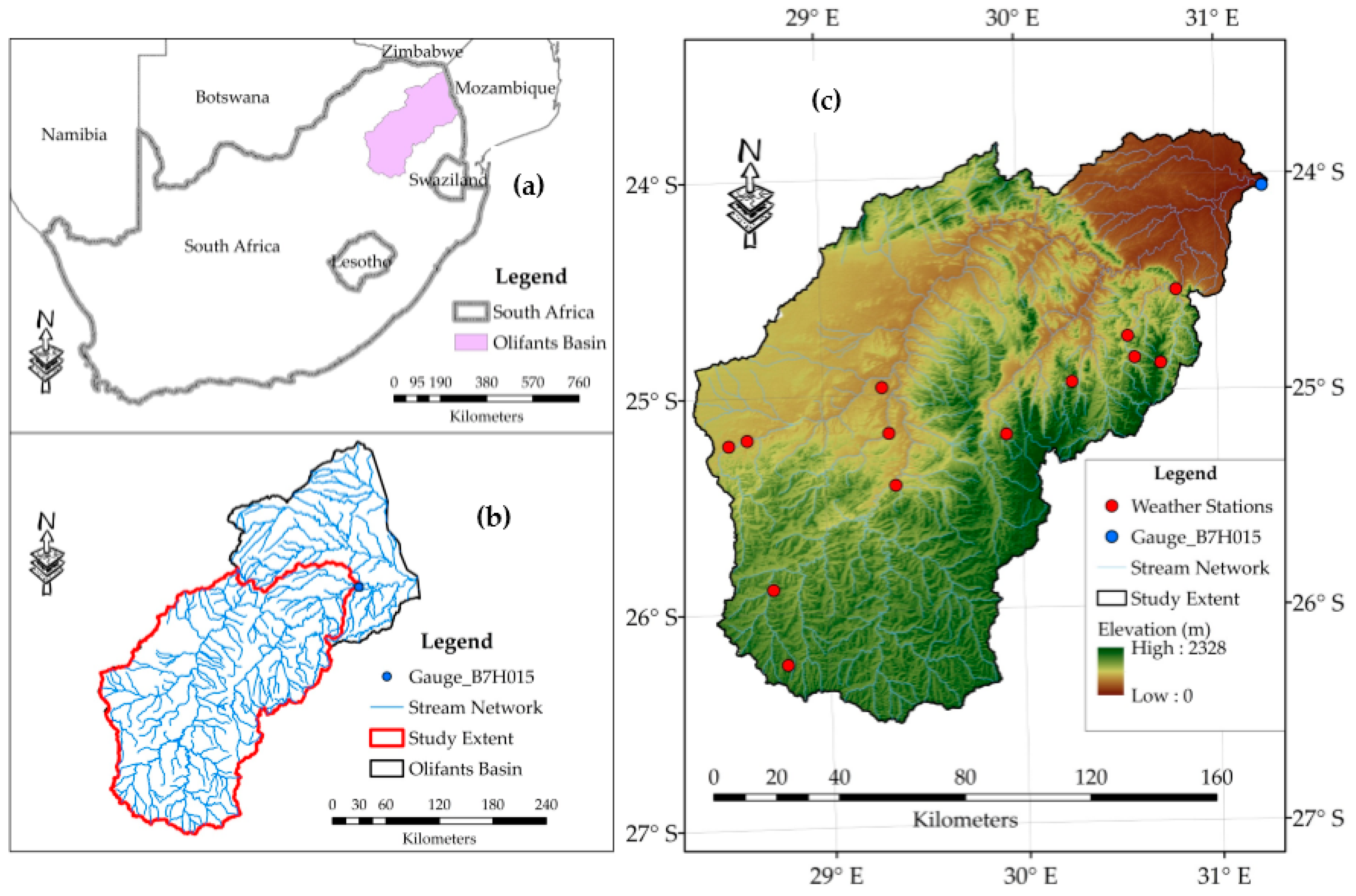
2.1. Study Location

The water stressed Olifants Basin located in the north-eastern part of South Africa was used as a case study. The newly modified Olifants Basin which is in accordance with the National Water Resource Strategy 2 (NWRS-2) [24] drains a total area of 73.7 × 10³ km² with the Olifants River traversing roughly 770 km before flowing into the Massingire dam in Mozambique. The basin spans between latitudes 22.6° S–26.5° S and longitudes 28.3° E–31.9° E. However, this study limits its investigations to the area extending from the upper Olifants to gauge station B7H015 (Figure 1) which drains an area of approximately 50,000 km². The main tributaries of the Olifant are the Wilge, Moses, Elands and Ga-Selati rivers on the left bank and Klein Olifant, Steelpoort and Blyde rivers on the right bank. On the right bank, Steelpoort is the largest tributary draining an area of 7136 km² compared to the Elands on the left bank with a drainage area of 6148 km². Generally, the elevation of the basin ranges from 0 m to 2400 m above mean sea level (m a.s.l.). Rainfall is seasonal in the basin, occurring during the months of October to April with appreciable spatio-temporal variability. The mean annual precipitation (MAP) is documented by Gyamfi et al. [25] to be 664 mm with peaks in January. Temperatures range from 18 °C to 34 °C in summer and 5 °C to 26 °C in winter. The basin is characterized by five major soil types namely; cambic arenosols, chromic luvisols, chromic vertisols, orthic acrisols and rhodic ferralsols [26]. Dominantly, land uses of the Olifants Basin consist of agriculture lands, built up areas and vegetation. According to McCartney et al. [27], agriculture forms an essential land use type with most activities centered on commercial and subsistence agriculture. In the northern and eastern sections of the basin are located small amounts of inland tropical forest with urban and agricultural expansion oriented in the southern and middle sections.

2.2. Model Selection and Description

The Soil and Water Assessment Tool (SWAT) was selected to assess the impacts of LULCs on the hydrology of the Olifants Basin. The SWAT model is a continuous, long-term, physically based distributed model considered one of the most suitable models for the simulation of land use impacts on water, agricultural pollutants and sediment in large complex watersheds [28,29]. The basic operational unit of the model is the hydrologic response unit (HRU) which consists of an area of homogenous land use, management and soil characteristics. The HRUs are nested within sub-basins and hence simulations are aggregated at the HRUs and then unto the sub-basins. Hydrological components simulated within the model include surface runoff, evapotranspiration, percolation, lateral flow, return flow, transmission losses and ponds [29]. SWAT is capable of integrating different spatial data, thus making it versatile in the area of watershed management and water resources planning in particular. For further reading on the SWAT model, one is referred to Arnold et al. [29] and online resource at http://swat-model.tamu.edu/.

2.3. Model Inputs

The input data required to run the SWAT model includes a Digital Elevation Model (DEM), digital soil data, digital land use and land cover maps, and climate data. The DEM (see Figure 1c) was a 3 arc second (90 m × 90 m) pixel resolution Shuttle Radar Topography Mission (SRTM) DEM, downloaded from the Consortium for Spatial Information of the Consultative Group of International Agricultural Research (CGIAR–CSI). Soil data and information on related soil properties were obtained from the Food and Agriculture Organization (FAO) soil map [26]. The LULC data for three time periods (2000, 2007 and 2013) used in the assessment of the impacts of LULC change on hydrology was obtained through a supervised land use classification of Landsat 7 Enhanced Thematic Mapper Plus (ETM+) images. The cloud free images of spatial resolution 30 m were downloaded from the United States Geological Survey database and are available at http://glovis.usgs.gov/.

Table 1. Details of Landsat 7 Enhanced Thematic Mapper Plus (ETM+) Images used for classification.

Acquisition Date	Path	Row	Image ID
3 June 2000	169	077	LE71690772000155SGS00
3 June 2000	169	078	LE71690782000155SGS00
23 April 2000	170	077	LE71700772000114SGS01
23 April 2000	170	078	LE71700782000114SGS01
22 May 2007	169	077	LE71690772007142ASN00
23 June 2007	169	078	LE71690782007174ASN00
13 May 2007	170	077	LE71700772007133ASN00
18 September 2007	170	078	LE71700782007261ASN00
7 June 2013	169	077	LE71690772013158ASN00
6 May 2013	169	078	LE71690782013126ASN00
14 June 2013	170	077	LE71700772013165ASN00
14 June 2013	170	078	LE71700782013165ASN00

details the attribute of the images for each epoch. The Scan Line Corrector (SLC) off data gaps in the acquired images were filled using SLC-off corrected data. Following gap filling and radiometric correction, images were classified into five level 1 classes (Figure 2) using ERDAS Imagine, version 14.0. The classification scheme developed by Anderson et al. [30] for the interpretation of remote sensor data was adopted in this study with details presented in

Table 2. Land cover classification scheme according to Anderson et al. [30].

Land Cover Class	Description
Rangeland	Herbaceous, shrub and brush and mixed rangeland
Water	Lakes, reservoirs, stream
Agricultural lands	Crop fields and pastures
Forest	Deciduous, evergreen and mixed forest
Urban/Built up	Residential, commercial services, industrial, transportation, communications, mixed urban or built up lands

. Climatic data including daily rainfall, maximum and minimum temperatures at thirteen weather stations were obtained from the South African Weather Service (SAWS) for the period between 1980 and 2013. Missing data in historical rainfall and temperature records were interpolated using the method proposed by Di Luzio et al. [31].

2.4. Model Calibration and Validation

The model was calibrated (1988–2001) and validated (2002–2013) using monthly stream flow data from gauge station B7H015. The first 8 years prior to 1988 were used as a warm up period to mitigate unknown initial conditions. Sensitive parameters to streamflow with their fitted values (

Table 3. Calibrated parameters for stream flow with sensitivity ranking (t-stat).

Parameter	Description	Range	Fitted Value	t-Stat (Absolute Values)
CN2	Runoff curve number	35–98	65 *	37.72
ALPHA_BNK	Base flow alpha factor for bank storage	0–1	0.39	6.97
ESCO	Soil evaporation compensation factor	0–1	0.67	5.57
SOIL_AWC	Soil available water capacity	0–1	0.2	4.13
GW_DELAY	Groundwater delay (days)	0–500	345	3.02
GW_REVAP	Groundwater “revap” coefficient	0.02–0.2	0.15	2.34

Notes: * Average basin value.

) were adapted from Gyamfi et al. [32]. The model performance was evaluated using four objective functions namely; coefficient of determination (R²), Nash–Sutcliffe efficiency (NSE), Root Mean Square Error (RMSE) observations standard deviation ratio (RSR) and percent bias (PBIAS). Three of the objective functions (NSE, PBIAS, RSR) for the calibrated and validated SWAT model were compared to the performance statistics ratings (

Table 4. General performance ratings for recommended statistics for monthly time step *.

Performance Rating	PBIAS (%)	RSR	NSE
Very good	$\mathrm{PBIAS}<\pm 10$	0.00 $\le \mathrm{RSR}\le 0.50$	0.75 $<\mathrm{NSE}\le 1.00$
Good	$\pm 10\le \mathrm{PBIAS}<\pm 15$	0.50 $\le \mathrm{RSR}\le 0.60$	0.65 $<\mathrm{NSE}\le 0.75$
Satisfactory	$\pm 15\le \mathrm{PBIAS}<\pm 25$	0.60 $\le \mathrm{RSR}\le 0.70$	0.50 $<\mathrm{NSE}\le 0.65$
Unsatisfactory	$\mathrm{PBIAS}\ge \pm 25$	$\mathrm{RSR}>0.70$	$\mathrm{NSE}\le 0.50$

Notes: * PBIAS: Percent bias; RSR: RMSE observation standard deviation ratio; NSE: Nash-Sutcliffe efficiency.

) for monthly time steps proposed by Moriasi et al. [33] to determine the performance of the model. Generally, a model is considered acceptable if the R² is greater than 0.5.

• Coefficient of determination (R²): It measures the proportional variation in the simulated variable explainable by the observed variable and gives an indication of the linear relationship between the simulated and observed variables. R² is calculated as follows:

  $${\mathrm{R}}^2={\left[\frac{{\displaystyle {\sum }_{\mathrm{i}=1}^{\mathrm{n}}\left({\mathrm{O}}_{\mathrm{i}}-{\mathrm{S}}_{\mathrm{i}}\right)\left({\mathrm{S}}_{\mathrm{i}}-\overline{\mathrm{S}}\right)}}{{\left({\displaystyle {\sum }_{\mathrm{i}=1}^{\mathrm{n}}{\left({\mathrm{O}}_{\mathrm{i}}-\overline{\mathrm{O}}\right)}^2}\right)}^{0.5}{\left({\displaystyle {\sum }_{\mathrm{i}=1}^{\mathrm{n}}{\left({\mathrm{S}}_{\mathrm{i}}-\overline{\mathrm{S}}\right)}^2}\right)}^{0.5}}\right]}^2$$

  (1)
• Nash–Sutcliffe efficiency (NSE): This statistic determines the relative magnitude of the residual variance compared to the observed data variance. NSE ranges from −$\infty$ to 1, where 1 denotes perfect agreement between simulated and observed variables. NSE is formulated as:

  $$\mathrm{NSE}=1-\frac{{\displaystyle {\sum }_{\mathrm{i}=1}^{\mathrm{n}}{\left({\mathrm{O}}_{\mathrm{i}}-{\mathrm{S}}_{\mathrm{i}}\right)}^2}}{{\displaystyle {\sum }_{\mathrm{i}=1}^{\mathrm{n}}{\left({\mathrm{O}}_{\mathrm{i}}-\overline{\mathrm{O}}\right)}^2}}$$

  (2)
• RMSE observations standard deviation ratio (RSR): RSR standardizes the root mean square error (RMSE) using the observation standard deviations. It is calculated as:

  $$\mathrm{R}\mathrm{S}\mathrm{R}=\frac{\mathrm{RMSE}}{{\mathrm{STD}}_{\mathrm{obs}}}=\frac{\sqrt{{\displaystyle {\sum }_{\mathrm{i}=1}^{\mathrm{n}}{\left({\mathrm{O}}_{\mathrm{i}}-{\mathrm{S}}_{\mathrm{i}}\right)}^2}}}{\sqrt{{\displaystyle {\sum }_{\mathrm{i}=1}^{\mathrm{n}}{\left({\mathrm{O}}_{\mathrm{i}}-\overline{\mathrm{O}}\right)}^2}}}$$

  (3)
• Percent Bias (PBIAS): PBIAS is a measure of how much (in percentage) the observed variable is either underestimated or overestimated. It is calculated as shown:

  $$\mathrm{PBIAS}=\frac{{\displaystyle {\sum }_{\mathrm{i}=1}^{\mathrm{n}}\left({\mathrm{O}}_{\mathrm{i}}-{\mathrm{S}}_{\mathrm{i}}\right)}}{{\displaystyle {\sum }_{\mathrm{i}=1}^{\mathrm{n}}{\mathrm{O}}_{\mathrm{i}}}}\times 100\%$$

  (4)

  where ${\mathrm{O}}_{\mathrm{i}}$ is the observed variable, ${\mathrm{S}}_{\mathrm{i}}$ is the simulated variable, $\overline{\mathrm{O}}$ is the mean of the observed variable, $\overline{\mathrm{S}}$ is the mean of the simulated variable, n is the number of observations under consideration, RMSE is the root mean square error, ${\mathrm{STD}}_{\mathrm{obs}}$ is the standard deviation of the observed variable.

2.5. Model Application

To assess the impacts of LULC on the hydrology of the Olifants Basin, the “fix-changing” method was used [4,9,34,35,36]. With this method, the calibrated model was run for each of the land use maps (2000, 2007 and 2013) from January 1988 to December 2013 whilst keeping constant the DEM, climatological parameters and soil data. Simulated results were further used to evaluate the impact of LULCs on hydrological components at the basin and sub-basinal scales. The changes observed in the hydrological components were mapped out at the sub-basinal scale using ArcGIS 10.2 to aid in decision making process.

2.6. Statistical Analysis

Evaluation of the impacts of LULC on hydrology was done by first comparing the average annual basin values for each of the land use scenarios. A bivariate correlation analysis using the Pearson’s pair-wise correlation matrix was used to establish a relationship between independent and dependent variables. Independent variables constituted the changes in four LULC classes (i.e., agriculture, rangeland, urban and forest) whiles the dependent variables were made of changes in four hydrological components (i.e., Surface runoff, Evaporation, Water Yield and Lateral flow variables). Further, the impacts of LULC on hydrologic responses were examined through a stepwise multi-regression analysis using simulated results for 2000 and 2013 land use scenarios. Initially, a check for normality with the Shapiro–Wilk (S–W) normality test indicated that the independent samples were not from a normal distribution population (S–W < 0.96; p < 0.05). As a result, the affected independent variables were log transformed to achieve a normally distributed population where necessary. A further check for multicollinearity on the log transformed independent variables proved the non-existence of collinearity with variance inflation factor (VIF) ranges of 1.72–3.00. Statistical Package for Social Sciences (SPSS) 20.0 (International Business Machines (IBM), SPSS, Chicago, IL, USA) was used for the multi-regression analysis and MS excel for graphical output presentation. ArcGIS 10.2 was used in mapping out the spatio-temporal changes observed in the hydrologic responses of the Olifants Basin to LULC change.

3. Results and Discussion

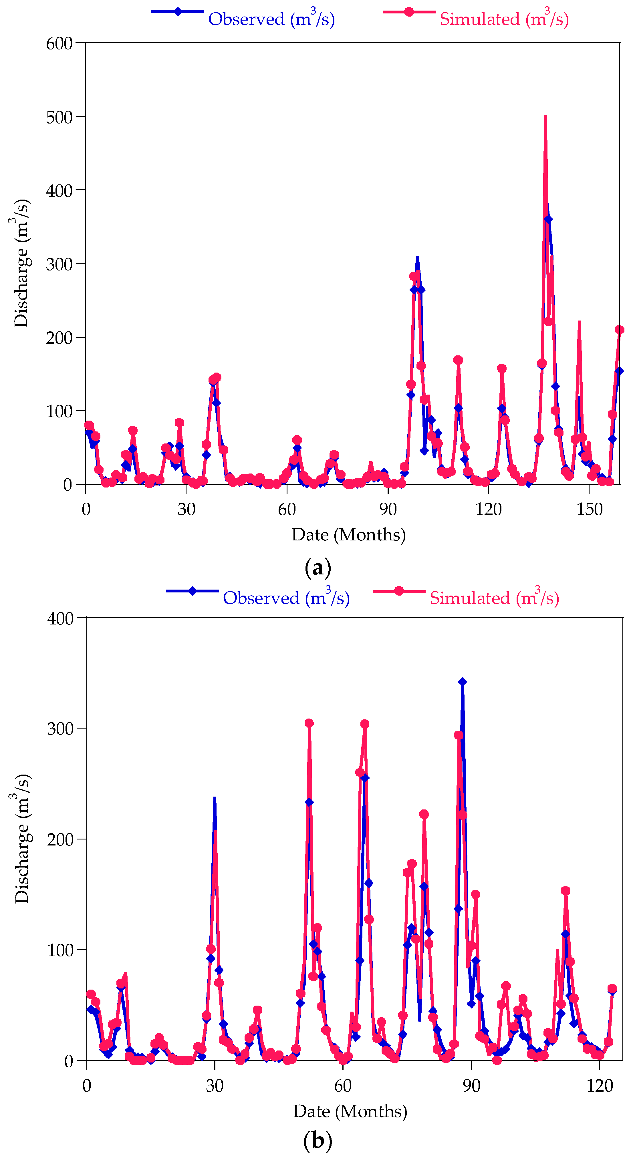
3.1. Calibration and Validation of the SWAT Model

The simulated and observed streamflow for the calibration period (January 1988–December 2001) and the validation period (January 2002–December 2013) are compared in Figure 3. A good match is revealed between the simulated and observed streamflow. The performance statistics values are shown in

Table 5. Monthly time step calibration and validation performance statistics.

Model Stage	Evaluation Statistics *
	R2	NSE	RSR	PBIAS (%)
Calibration (1988–2001)	0.89	0.88	0.34	−11.49
Validation (2002–2013)	0.78	0.67	0.57	−20.69

Notes: * R²: Coefficient of determination; NSE: Nash-Sutcliffe efficiency; RSR: RMSE observation standard deviation ratio; PBIAS: Percent bias.

. From Table 5, NSE and R² values for both the calibration and validation period are greater than 0.6, and the PBIAS values are in the range of ±10%, indicating a good model performance [33]. Notwithstanding the satisfactory model performance, SWAT overestimated the observed streamflow by 11.49% during the calibration period and by 20.69% in the validation period. This is exemplified in the negative values of PBIAS.

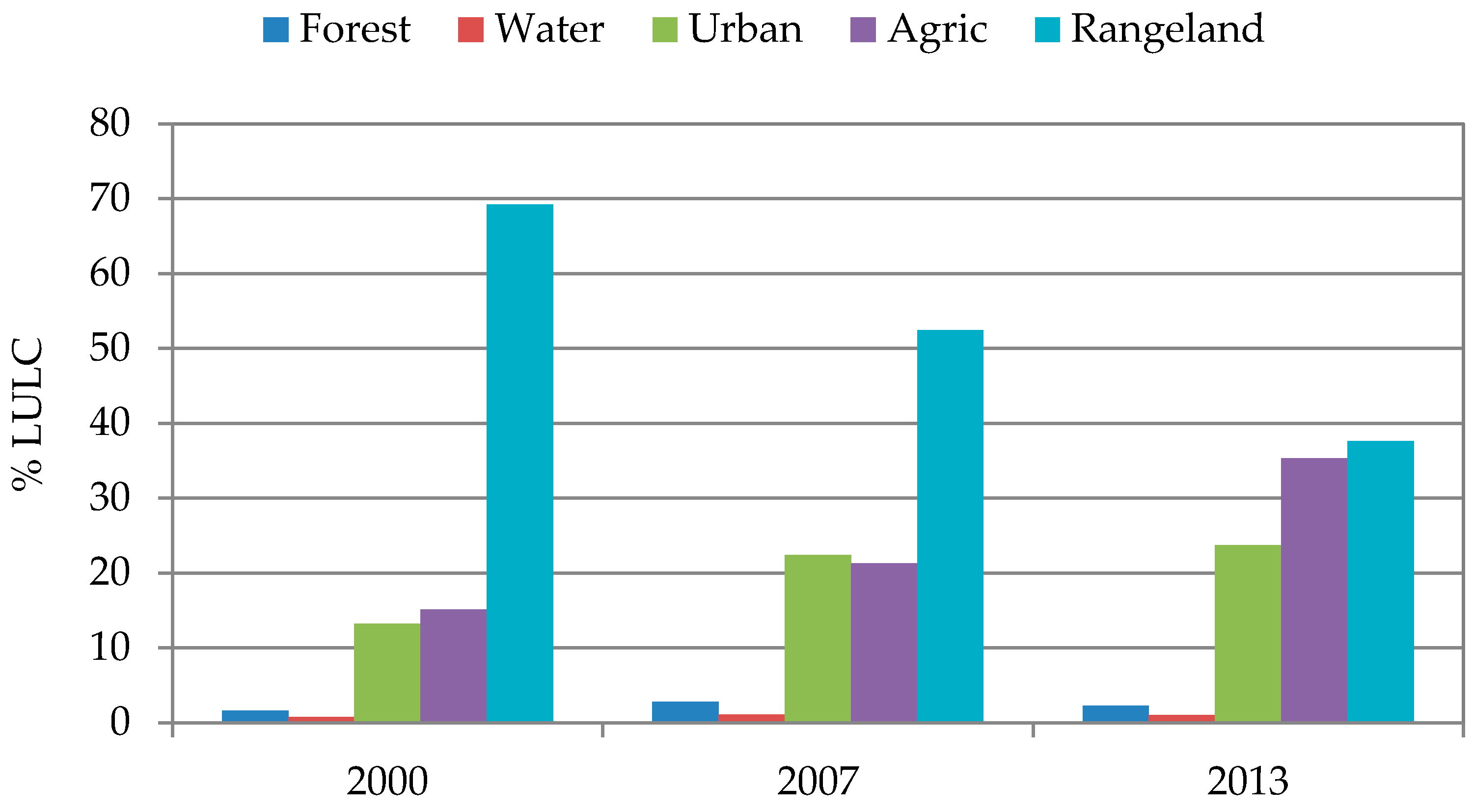
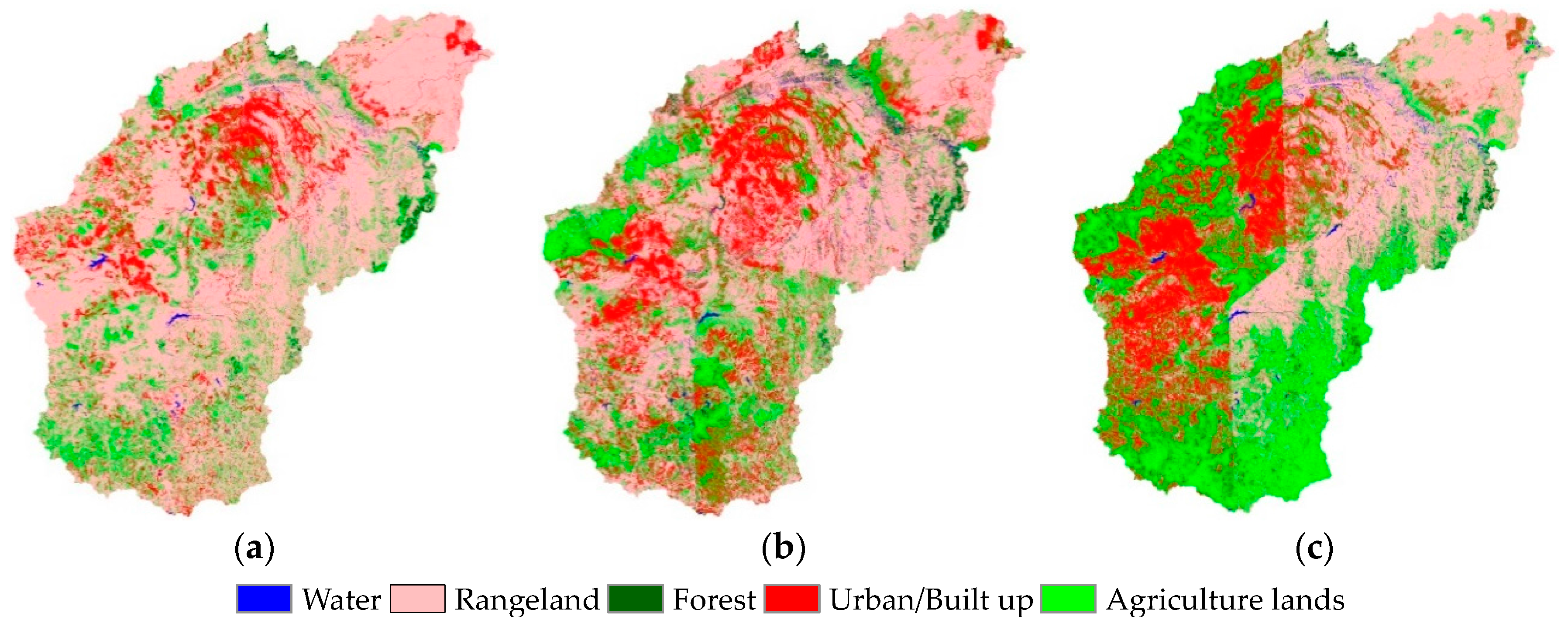
3.2. Land Use Change Detection

LULC observed in the Olifants basin for the period 2000 to 2013 are shown in Figure 4 with classification accuracies presented in

Table 6. Summary of Landsat classification accuracies (%) for 2000, 2007 and 2013.

Land Cover Class	2000		2007		2013
	Producers’	Users’	Producers’	Users’	Producers’	Users’
Urban/Built up	65.63	80.77	87.50	94.23	84.00	84.00
Rangeland	97.50	89.14	97.69	88.81	89.01	82.65
Water	100.0	100.00	100.00	100.00	100.00	85.71
Agriculture	76.36	87.50	86.27	86.27	88.54	88.54
Forest	71.43	100.00	41.18	87.50	30.77	80.00
Overall accuracy	88.28		89.45		85.16
Kappa	77.43		83.00		78.28

. The accuracy statistics were estimated from generated error matrices of the classified images. Evidently, a satisfactory land use classification was achieved with overall accuracy statistics of 88.28%, 89.45% and 85.16% for 2000, 2007 and 2013 respectively. The overall accuracy statistics obtained in the classification process are in conformance with the minimum threshold of 85% suggested by Anderson et al. [30] for land use classification. The kappa statistics were respectively 77.43%, 83.00% and 78.28% for 2000, 2007 and 2013 classified images which are also in accordance with acceptable ranges of 61%–99% [37]. From Figure 4, it is apparent that changes occurred in all land use classes. Nonetheless, most significant changes were observed in three land use classes, namely urban areas, agricultural lands and rangelands. Urban and agricultural areas continually increased for all the years under review. Urban area extent of 13.2% in 2000 increased to 22.4% in 2007. Urban areas gradually increased again from 22.4% in 2007 to 23.7% in 2013. Similarly, from 2000 to 2007, agricultural areas increased from 15.2% to 21.3%. Further expansion in agriculture lands were observed, increasing from 21.3% in 2007 to 35.3% in 2013. Unlike agriculture and urban areas, rangeland continually decreased from 69.2% to 52.4% between the period 2000 to 2007. By the end of 2013, rangeland had decreased from 52.4% in 2007 to 37.6% making it the land use type to have received the most significant reduction for the period under study. The reduction in rangeland was mainly due to its conversion into agricultural and urban land uses. This is exemplified in the southern portion of the basin where rangelands in 2000 had given way to agricultural activities in 2013 (see Figure 2). The urban sprawl is connected with the numerous industrial activities that are domiciled and much concentrated within the southern and middle portions of the basin [38].

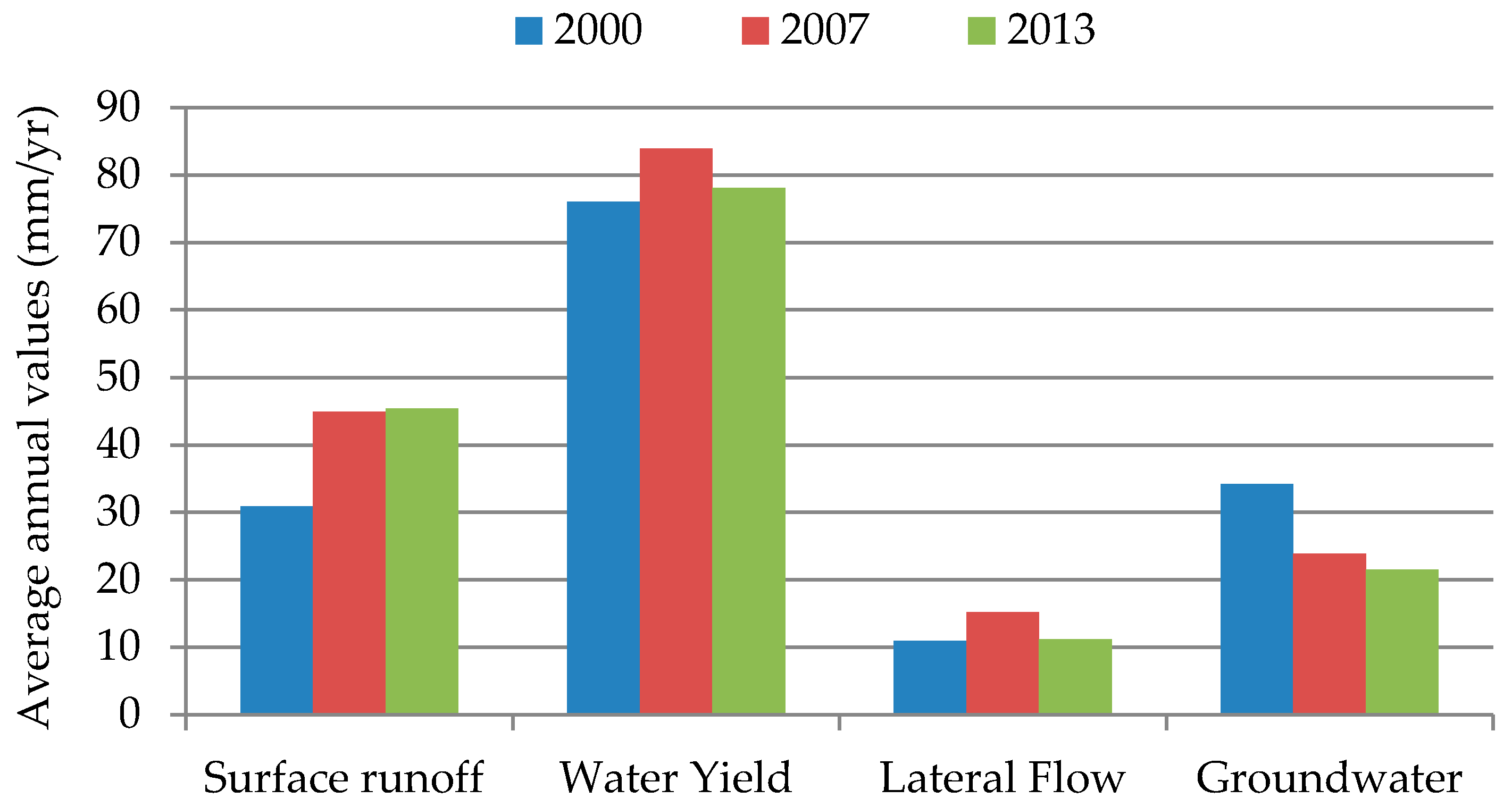
3.3. Hydrological Responses to Different Land Use Scenarios at the Basinal Scale

The calibrated SWAT models were used to simulate the impact of LULC change on the hydrological responses of the Olifants Basin considering three different land use scenarios. The average annual values of four hydrological components (surface runoff, water yield, lateral flow and groundwater) are shown in Figure 5 and

Table 7. Changes in four hydrological components based on three land use change scenarios.

Hydrologic Component	LULC Scenario
	2000	2007	2013
Surface runoff (mm)	30.91	44.91	45.43
Water yield (mm)	76.04	83.92	78.11
Lateral flow (mm)	10.92	15.18	11.18
Groundwater (mm)	34.21	23.84	21.5
Evapotranspiration (mm)	518.40	546.60	531.40

. It is evident from Figure 5 and Table 7 that the utmost impact of LULC change was on the amount of runoff generated. This finding is consistent with Ghaffari et al. [9] in which, among the three hydrologic components studied (streamflow, groundwater and baseflow), streamflow was the most affected by LULC changes. Compared to the LULC in 2000, the average annual surface runoff over the basin is 14.00 mm higher in 2007 and 14.52 mm higher in 2013: an increase of 45.3% and 46.9% respectively. Average water yield in 2000 was 76.00 mm, increasing to 83.92 mm with LULC in 2007 (increase of 10.4%). However, there was a reduction in average water yield by 2.7% in 2013. A similar trend as detected in water yield was evident for lateral flow. The average lateral flow increased from 10.92 mm with LULC in 2000 to 15.18 mm with LULC in 2007 (increase of 39.0%). With LULC of 2013, the average lateral flow reduced by 26.4% from 15.18 mm to 11.18 mm with LULC of 2007.

A unique trend of continuous groundwater decline was noticed (Figure 5 and Table 7). From 2000 to 2007, the annual groundwater recharge decreased by 10.37 mm (30.3%). A further decline in groundwater recharge of 12.71 mm (37.2%) was observed in 2013. A similar decline in groundwater recharge has been reported by other studies [3,9,39]. The declining trend seen in the average groundwater recharge can be attributed to increases in surface runoff, less soil infiltration and higher evapotranspiration. It is also the case that groundwater resources within the basin are sourced for several activities, including household water use, industrial uses, animal husbandry and irrigation [40,41]. A resulting effect of these uses of groundwater may account for the continuous decline in groundwater recharge due to overexploitation of the resource over the years. The reduction in groundwater recharge as depicted by the model results is indeed consistent with the findings of Calow and MacDonald [42] where they asserted that groundwater is a preferred source of water over surface water due to the high inter-annual variations in precipitation which tend to affect surface water availability. This is particularly the case in semi-arid environments in Africa and so is the case of the Olifants Basin [43].

A comparison of the variations in surface runoff under the three LULC change scenarios shows that the basin is under flashier flow regime influence which results in the conversion of rainfall to runoff. The increases in surface runoff are linked to the significant changes in watershed cover, resulting mainly from the conversion of rangeland to urban and agricultural areas (Figure 4) and consequently causing increases in impervious surface covers [44].

Findings from other studies indicate similar effects of urbanization on stream hydrology through flashier flow regimes [45,46,47]. Although surface runoff increased for all the LULC change scenarios, water yield reduced in 2013 probably due to the reduction in groundwater recharge and lateral flow. Baker and Miller [3] also found a similar relationship between increases in surface runoff and proportionate decline in groundwater recharge. In addition to simulating surface runoff, water yield and groundwater, the SWAT model also gave good predictions of evapotranspiration (ET). ET increased from 518.4 mm in 2000 to 546.6 mm in 2007 (an increase of 5.4%). Post 2007 saw a decline in ET from 546.6 mm to 531.4 mm in 2013 (decrease of 2.8%). The increases and decline in ET (Table 7) coincide with increases and decline in forest cover and water (Figure 4) for the same period under consideration. This is so because trees that make up forest generally have the ability to access soil moisture from greater depths for transpiration and also have greater canopy cover for interception of precipitation which eventually culminates into the higher observed ET [4].

3.4. Alterations in Water Balance Ratios

Water balance ratios provide a framework for the assessment of the partitioning of rainfall into different components based on changes in watershed conditions.

Table 8. Potential ratios of basin hydrology simulated on three LULC scenarios based on the hydrological year (October–September).

LULC Scenario	Water Balance Ratios *
	B/TF	SR/TF	SF/P	PC/P	DR/P	ET/P
2000	0.26	0.74	0.07	0.1	0.05	0.78
2007	0.25	0.75	0.09	0.05	0.04	0.82
2013	0.24	0.76	0.09	0.08	0.03	0.80

Notes: * B/TF: Baseflow/Total flow; SR/TF: Surface runoff/Total flow; SF/P: Streamflow/Precipitation; PC/P: Percolation/Precipitation; DR/P: Deep Recharge/Precipitation; ET/P: Evapotranspiration/Precipitation.

elucidates the water balance ratios for the Olifants Basin under three LULC change scenarios. The baseflow index (BFI) simulated by the model (Table 8) was compared with that obtained using the Web-based Hydrograph Analysis Tool (WHAT) on observed stream flow. Results from the WHAT analysis indicate that about 33% (0.33) of observed streamflow is made of baseflow and 67% (0.67) of surface runoff. Simulated results on the BFI, although not the same as those observed, indicated a closer range of 24%–26% (0.24–0.26) baseflow component of streamflow with a decline from 2000 to 2013. The decreasing orders of dominance in rainfall partitioning were evapotranspiration, stream flow, percolation and deep aquifer recharge. The simulated average annual evapotranspiration accounted for 78%–82% (ratios of 0.78–0.80) of basin-wide estimated precipitation, thus making evapotranspiration a key determining factor of water resources availability in the basin. This result is also consistent with the findings of Department of Water Affairs (DWA) [41] who stated that evapotranspiration in the Olifants Basin is approximately 70%. Schulze et al. [48] also alluded to the high incidence of evapotranspiration, terming it as the highest water consumer within the basin. Evapotranspiration was highest in the period from October to May and reached minimum values in July and August. The seasonal trend in evapotranspiration conforms to the general seasonality in rainfall within the basin.

Groundwater recharge constituted between 3% and 5% (ratios of 0.03–0.05) of basin-wide mean annual precipitation (MAP). Likewise, DWA [49] reported 3%–6% of MAP as contributions to groundwater recharge within the basin. The changes observed in the water balance ratios generally follow the trend of the impact of LULC changes on hydrological components already discussed.

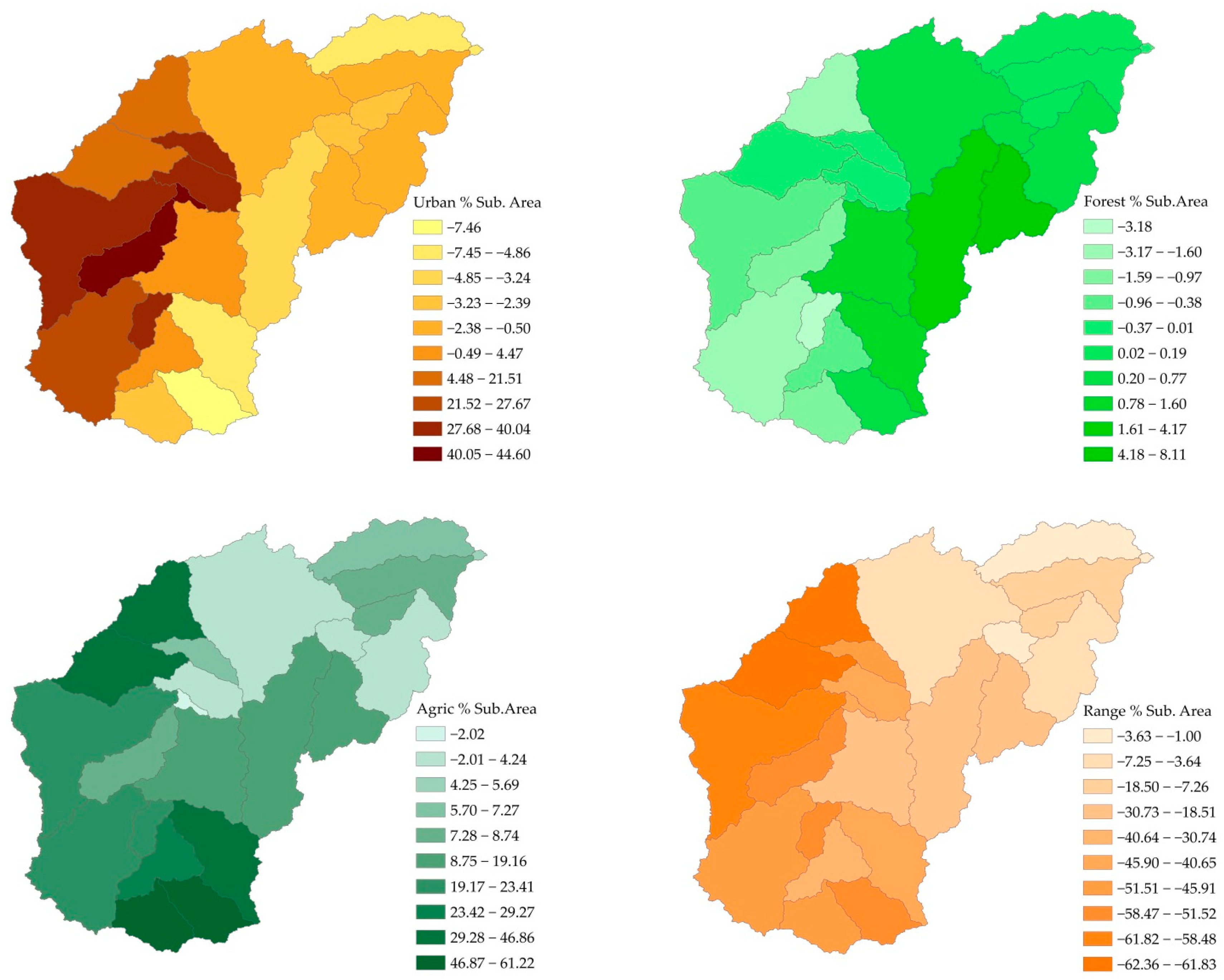
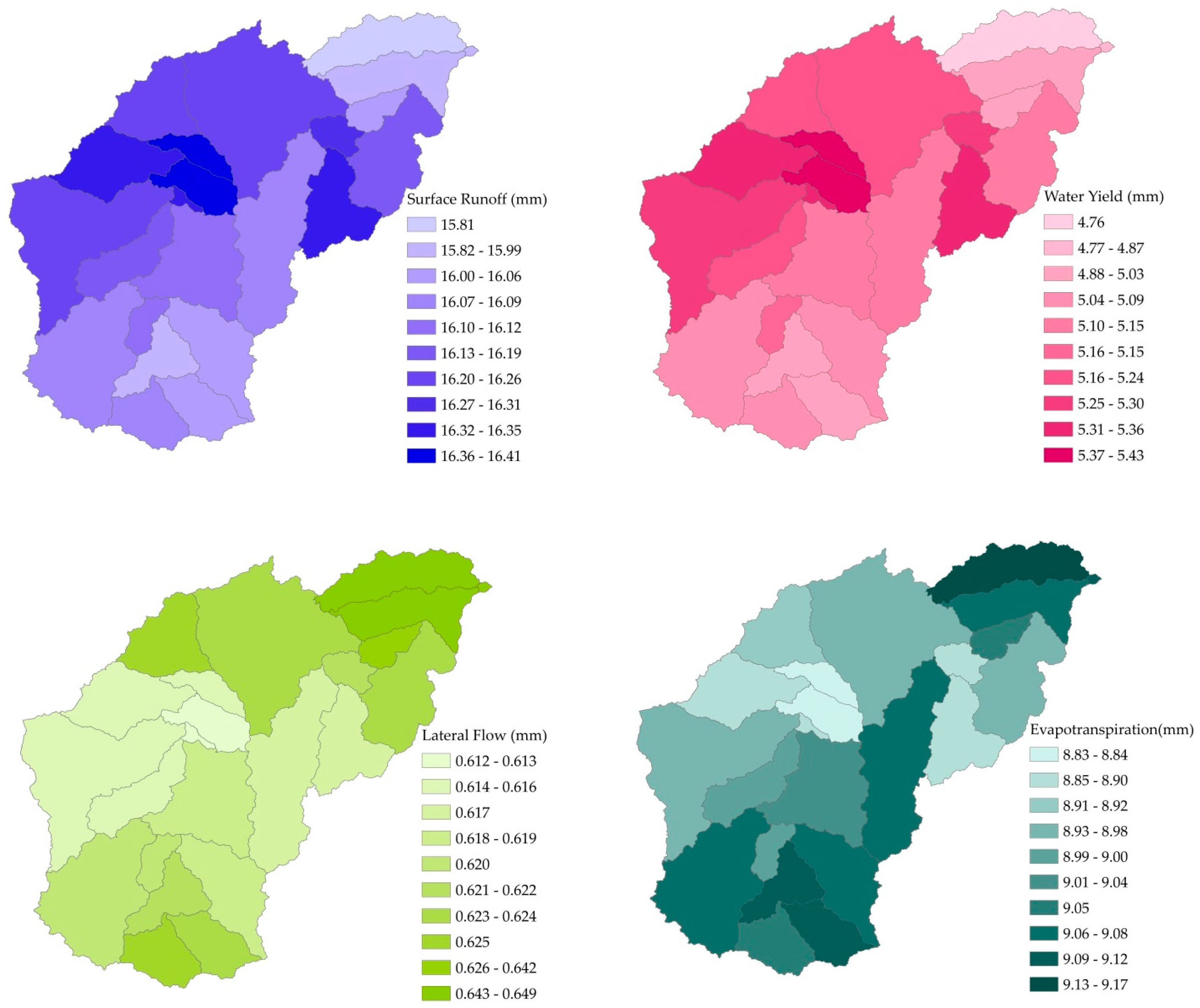
3.5. Contributions of Changes in Individual LULCs on Hydrological Components at the Sub-Basinal Scale

Shown in Figure 6 and Figure 7 are the spatial distribution of changes in four land use types (i.e., urban, agriculture, forest and rangeland) and four simulated hydrologic components (i.e., surface runoff, water yield, lateral flow and evapotranspiration) between 2000 and 2013. Urban expansion mainly occurred in the north-western and south-eastern part of the basin. Expansion in agriculture was observed to be high in the north-western and southern parts of the basin. The expansions in urban areas and agriculture were due to the invasion of rangelands. This is confirmed by the negative high correlation between urban, agriculture and rangelands (

Table 9. Bivariate Pearson correlation for changes in four LULC types and four hydrological components between 2000 and 2013 ^a. Bold numbers are for p < 0.05.

	SURQ	WYLD	ET	LAT Q	FRST	URHD	AGRL	RNGB
SURQ	1.00
WYLD	0.98	1.00
ET	−0.99	−0.96	1.00
LAT Q	−0.72	0.81	0.65	1.00
FRST	0.09	0.13	0.05	−0.15	1.00
URHD	0.88	0.82	−0.24	0.36	−0.44	1.00
AGRL	0.61	0.54	0.15	−0.31	0.00	0.43	1.00
RNGB	−0.15	−0.22	0.08	0.42	0.21	−0.85	−0.83	1.00

Notes: ^a SURQ: Surface Runoff; WYLD: Water Yield; ET: Evapotranspiration; LAT Q: Lateral Flow; FRST: Forest; URHD: Urban area; AGRL: Agriculture; RNGB: Rangelands.

). Increases in forest cover occurred mainly in the east of the basin. Although rangeland decreased across all the sub-basins, the reduction was predominant at the north-western section of the basin, buttressing the conversion of this land use type to urban and agricultural areas.

The most significant increases in hydrologic components of surface runoff and water yield occurred mainly in the north-western part of the basin, corresponding to a large extent with the spatial distribution in urban and agricultural expansions. This is explicit in the positive correlation surface runoff has with urban and agriculture areas (Table 9). Similarly, water yield correlates positively with urban and agricultural areas. Generally, evapotranspiration (ET) increased across all the sub-basins, however significant increases were observed in the northern corner, eastern and south-eastern part of the basin. The spatial distribution of the significant increases in ET somewhat matches fairly with the areas detected to be covered by forest and agriculture lands. Trees and plants in forest and agriculture lands take up much water for transpiration and photosynthetic purposes, which may result in increases in ET. Although major increases in ET occurred in forest and agricultural areas, the correlation analysis (Table 9) suggests a weak relationship between ET and all the land use types. This suggests that there is a more complex mechanism that controls changes in ET. ET is a key water availability determinant in the basin, as it negatively influences surface runoff and water yield (Table 9). Although lateral flow across sub-basins increased, the increase was marginal. The spatial distribution of lateral flow demonstrates predominant occurrence in the northern part of the basin, which happens to be the downstream end. This may possibly be explained by the fact that more runoff from upstream after fulfilling transmission and storage losses are channeled into lateral flow.

To examine the effects of each land use type on hydrologic response, all four land use types were regressed stepwise against each of the four hydrologic components (i.e., surface runoff, water yield, lateral flow and evapotranspiration) and the results are summarized in

Table 10. Responses of four hydrologic components to individual LULC types (predictors), values represent partial R² with +/– indicating direction of influence.

Responses	Predictors				R2
	Urban	Agric	Forest	Rangeland
Surface runoff	0.48(+)	0.13(+)			0.61
Water yield	0.54(+)	0.13(+)		0.08(−)	0.75
Lateral flow		0.14(+)		0.53(+)	0.67
ET	0.48(+)		0.15(+)		0.63

Notes: Bold numbers are for p < 0.05 for all F tests.

. Alterations in surface runoff were mainly caused by expansions in urban and agriculture areas. Cumulatively, urban and agricultural expansion explained 61% of the total variance observed in surface runoff. Urban expansion was found to be the strongest positive contributor to changes in surface runoff with partial variance of 48%. Comparable to surface runoff, urban and agriculture expansion together explained 75% of the total variance in water yield from 2000 to 2013. Of the two LULC types, urban expansion exhibited the strongest contribution to changes in water yield with partial variance of 54%. Surface runoff constitutes approximately 76% of water yield, hence LULC types that influenced surface runoff generation were to be expected to influence water yield as well. However, the magnitudes of the influence were different as shown in Table 10. Previous studies found urbanization and agriculture expansion to have a greater influence on surface runoff [4,23].

Lateral flow was mostly influenced by agriculture and rangelands with the latter having a greater influence of 53% of the total variance observed in lateral flow. The cumulative variance in lateral flow resulting from agriculture and rangelands was 67%. Rangelands, unlike forest cover, have low transpiration demands, thus causing more water availability compared to increases in forest cover. Subsequently, lateral flows may be enhanced after transmission losses are satisfied. This explains the positive effects that rangelands have on lateral flow. A similar explanation holds true for the positive relation between agriculture lands and lateral flow, comparing the former with forest cover. Changes in urban and forest cover were identified as the strongest contributor (positive) to the changes in ET from 2000 to 2013. The positive impact of urbanization and forest cover on ET is expected because urbanization increases surface runoff thus causing forest cover to abstract more water for transpiration purposes. Increases in ET from 2000 to 2013 are attributed to the increases in urban and forest covers.

Elsewhere, ET is reported to have reduced by 69% and 81% when forest cover was replaced with barley and pasture respectively [11]. The reasons ascribed to the reduction in ET were linked to the shorter vegetation period of barley and pasture compared to forest resulting in less water uptake for transpiration and eventually culminating in ET reduction. Equally, in the upper San Pedro watershed in USA, Nie et al. [23] found ET to be less in areas covered by grassland than in areas covered by shrubs and woodland and attributed the difference to the relatively low transpiration demands of grassland compared to shrubs and woodland. These findings suggest that ET is less in areas with low plants transpiration demands and vice versa. An implication of alterations in hydrological responses, especially in surface runoff generation, is felt on sediment yield dynamics as reported by Gyamfi et al. [50].

4. Conclusions

This paper investigated the hydrological responses of a semi-arid watershed to current land cover dynamics for the period from 2000 to 2013. The study quantified the magnitude and direction of variations in major hydrological components resulting from land use and land cover (LULC) changes by coupling hydrologic simulations in SWAT with a multi-regression analysis. The SWAT model demonstrated versatility in modelling the effects of LULC changes on watershed hydrology with satisfactory accuracy. Urbanization and agriculture expansion were dominant land use types and subsequently the highest contributors to the hydrodynamics of the study basin. A 31.6% decrease in rangeland with concomitant increases in agriculture lands (20.1%), urban areas (10.5%) and forest (0.7%) led to a 46.97% increase in surface runoff generation. Further analyses indicate urbanization as the strongest contributor to increases in surface runoff generation, water yield and evapotranspiration (ET). ET was found to be a key water availability determinant as it has a high negative impact on surface runoff and water yield. Increases in ET were linked to expansions in forest and urban areas. Urbanization and agriculture are considered as the most essential environmental factors influencing water resources of the basin with ET playing a major role. The output of the paper indicates the usefulness of SWAT as a decision support tool (DST) in evaluating the impacts of land use changes on water resources. It again emphasizes the need for the use of simplistic assessment methods and tools in investigating the impacts of dynamic environmental factors on water resources in order to aid in the adaptation of more pragmatic and sustainable water resources strategies.

References

1. Githui, F.; Mutua, F.; Bauwens, W. Estimating the impacts of land cover change on runoff using the soil and water assessment tool (SWAT): Case study of Nzoia catchment, Kenya. Hydrol. Sci. J. 2010, 54, 899–908. [Google Scholar] [CrossRef]
2. Cai, T.; Li, Q.; Yu, M.; Lu, G.; Cheng, L.; Wei, X. Investigation into the impacts of land use change on sediment yield characteristics in the upper Huaihe River basin, China. Phys. Chem. Earth B 2012, 53–54, 1–9. [Google Scholar] [CrossRef]
3. Baker, T.J.; Miller, S.N. Using the Soil and Water Assessmnent Tool (SWAT) to assess land use impact on water resources in an East African watershed. J. Hydrol. 2013, 486, 100–111. [Google Scholar] [CrossRef]
4. Yan, B.; Fang, N.F.; Zhang, P.C.; Shi, Z.H. Impacts of land use change on watershed streamflow and sediment yield: An assessment using hydrologic modelling and partial least squares regression. J. Hydrol. 2013, 484, 26–37. [Google Scholar] [CrossRef]
5. Woldesenbet, T.A.; Elagib, N.A.; Ribbe, L.; Heinrich, J. Hydrological responses to land use/cover changes in the source region of the Upper Blue Nile Basin, Ethiopia. Sci. Total Environ. 2016, in press. [Google Scholar] [CrossRef] [PubMed]
6. Singh, R.; Van Werkhoven, K.; Wagener, T. Hydrological impacts of climate change in gauged and ungauged watersheds of the Olifants basin: A trading-space-for-time approach. Hydrol. Sci. J. 2014, 59, 29–55. [Google Scholar] [CrossRef]
7. Uhlenbrook, S.; McDonnell, J.; Leibundgut, C. Run-off generation and implications for river basin modelling special issue. Hydrol. Process. 2003, 17, 197–198. [Google Scholar] [CrossRef]
8. Wang, S.; Kang, S.; Zhang, L.; Li, F. Modelling hydrological response to different land use and climate change scenarios in the Zamu River basin of the northwest China. Hydrol. Process. 2008, 22, 2502–2510. [Google Scholar] [CrossRef]
9. Ghaffari, G.; Keesstra, S.; Ghodousi, J.; Ahmadi, H. SWAT–Simulated hydrological impact of land use change in the Zanjanrood Basin, Northwest Iran. Hydrol. Process. 2010, 24, 892–903. [Google Scholar] [CrossRef]
10. Karvonen, T.; Koivusalo, H.; Jauhiainen, M. A hydrological model for predicting runoff from different land use areas. J. Hydrol. 1999, 217, 253–265. [Google Scholar] [CrossRef]
11. Fohrer, N.; Haverkamp, S.; Eckhardt, K.; Frede, H.G. Hydrologic response to land use changes on the catchment scale. Phys. Chem. Earth B 2001, 26, 577–582. [Google Scholar] [CrossRef]
12. Felix, N.; Simon, S.; Markus, W.A. Process based assessment of the potential to reduce flood runoff by land use change. J. Hydrol. 2002, 267, 74–79. [Google Scholar]
13. Niraula, R.; Meixner, T.; Norman, L. Determining the importance of model calibration for forecasting absolute/relative changes in streamflow from LULC and climate changes. J. Hydrol. 2015, 522, 439–451. [Google Scholar] [CrossRef]
14. Wu, Y.; Liu, S.; Qiu, L.; Sun, Y. SWAT-DayCent coupler: An integration tool for simultaneous hydro-biogeochemical modeling using SWAT and DayCent. Environ. Model. Softw. 2016, 86, 81–90. [Google Scholar] [CrossRef]
15. Tuo, Y.; Duan, Z.; Disse, M.; Chiogna, G. Evaluation of precipitation input for SWAT modeling in Alpine catchment: A case study in the Adige river basin (Italy). Sci. Total Environ. 2016, 573, 66–82. [Google Scholar] [CrossRef] [PubMed]
16. Muenich, R.L.; Chaubey, I.; Pyron, M. Evaluating potential water quality of a fish regime shift in the Wabash River using the SWAT model. Ecol. Model. 2016, 340, 116–125. [Google Scholar] [CrossRef]
17. Zhang, X.; Ren, L.; Kong, X. Estimating spatiotemporal varaibility and sustainability of shallow groundwater in a well-irrigated plain of the Haihe River basin uisng SWAT model. J. Hydrol. 2016, 541, 1221–1240. [Google Scholar] [CrossRef]
18. Briak, H.; Moussadek, R.; Aboumaria, K.; Mrabet, R. Assessing sediment yield in Kalaya gauged watershed (Northern Morocco) using GIS and SWAT model. Int. Soil Water Conserv. Res. 2016, 4, 177–185. [Google Scholar] [CrossRef]
19. Stoll, S.; Franssen, H.; Butts, M.; Kinzelbach, W. Analysis of the impact of climate change on groundwater related hydrologicalfluxes: A multi-model approach including different downscaling methods. Hydrol. Earth Syst. Sci. 2011, 15, 21–38. [Google Scholar] [CrossRef] [Green Version]
20. Cuo, L.; Lettenmaier, D.P.; Mattheussen, B.V.; Storck, P.; Wiley, M. Hydrological prediction for urban watersheds with the distributed hydrology soil vegetation model. Hydrol. Process. 2008, 22, 4205–4213. [Google Scholar] [CrossRef]
21. Qi, S.; Sun, G.; Wang, Y.; McNulty, S.G.; Myers, J.A.M. Streamflow response to climate and landuse changes in a coastal watershed in North Carolina. Trans. ASABE 2009, 52, 739–749. [Google Scholar] [CrossRef]
22. Stathis, D.; Sapountzis, M.; Myronidis, D. Assessment of land use change effect on a design storm hydrograph using the SCS curve number method. Fresenius Environ. Bull. 2010, 19, 1928–1934. [Google Scholar]
23. Nie, W.; Yuan, Y.; Kepner, W.; Nash, M.S.; Jackson, M.; Erickson, C. Assessing impacts of land use and land cover changes on hydrology for the upper San Pedro watershed. J. Hydrol. 2011, 407, 105–114. [Google Scholar] [CrossRef]
24. Department of Water Affairs. Draft National Water Resource Strategy 2 (NWRS 2): Managing Water for an Equitable and Sustainable Future; DWA: Pretoria, South Africa, 2012.
25. Gyamfi, C.; Ndambuki, J.M.; Salim, R.W. A historical analysis of rainfall trend in the Olifants Basin in South Africa. Earth Sci. Res. 2016, 5, 129–142. [Google Scholar] [CrossRef]
26. Food and Agriculture Organization. Digital Soil Map of the World and Derived Soil Properties of the World; Food and Agricultural Organization of the United Nations: Rome, Italy, 2005. [Google Scholar]
27. McCartney, M.P.; Yawson, D.K.; Magagula, T.F.; Seshoka, J. Hydrology and Water Resources Development in the Olifants River Catchment: Working Paper 76; International Water Management Institute (IWMI): Colombo, Sri Lanka, 2004. [Google Scholar]
28. Arnold, J.G.; Fohrer, N. Current capabilities and research opportunities in applied watershed modeling. Hydrol. Process. 2005, 19, 563–572. [Google Scholar] [CrossRef]
29. Arnold, J.G.; Srinivasan, R.; Muttiah, R.S.; Williams, J.R. Large area hydrologic modeling and assessment—Part 1: Model development. J. Am. Water Res. Assoc. 1998, 34, 73–89. [Google Scholar] [CrossRef]
30. Anderson, J.R.; Hardy, E.E.; Roach, J.T.; Witmer, W.E. A Land Use and Land Cover Classification System for Use with Remote Sensor Data; USGS (United States Geological Survey): Washington, VI, USA, 1976; Volume 964, pp. 138–145.
31. Di Luzio, M.; Johnson, G.L.; Daly, C.; Eischeid, J.K.; Arnold, J.G. Constructing retrospective gridded daily precipitation and temperature datasets for the conterminous United States. J. Appl. Meteorol. Clim. 2008, 47, 475–497. [Google Scholar] [CrossRef]
32. Gyamfi, C.; Ndambuki, J.M.; Salim, R.W. Application of SWAT Model to the Olifants Basin: Calibration, Validation and Uncertainty Analysis. J. Water Res. Prot. 2016, 8, 397–410. [Google Scholar] [CrossRef]
33. Moriasi, D.N.; Arnold, J.G.; Van Liew, M.W.; Bingner, R.L.; Harmel, R.D.; Veith, T.L. Model evaluation guidelines for systematic quantification of accuracy in Watershed Simulations. Trans. ASABE 2007, 50, 885–900. [Google Scholar] [CrossRef]
34. Wang, G.; Xia, J.; Chen, J. Quantification of the effects of climate variations and human activities on runoff by a monthly water balance model: A case study of the Chaobai River Basin in Northern China. Water Res. 2009, 45, W00A11. [Google Scholar] [CrossRef]
35. Tang, L.H.; Yang, D.W.; Hu, H.P.; Gao, B. Detecting the effect of land use change on streamflow, sediment and nutrient losses by distributed hydrological simulation. J. Hydrol. 2011, 409, 172–182. [Google Scholar] [CrossRef]
36. Lin, B.; Chen, X.; Yao, H.; Chen, Y.; Liu, M.; Gao, L.; James, A. Analysis of landuse change impacts on catchment runoff using different time indicators based on SWAT model. Ecol. Indic. 2015, 58, 55–63. [Google Scholar] [CrossRef]
37. Viera, A.J.; Garrett, J.M. Understanding inter-observer agreement: The Kappa statistic. Fam. Med. 2005, 37, 360–363. [Google Scholar] [PubMed]
38. Department of Water Affairs. Development of a Reconciliation Strategy for the Olifants River Water Supply System: Summary Report; Report No. P WMA 04/B50/00/8310/2; DWA: Pretoria, South Africa, 2010.
39. Tripathi, M.P.; Panda, R.K.; Raghuwanshi, N.S. Development of effective management plan for critical subwatersheds using SWAT model. Hydrol. Process. 2005, 19, 809–826. [Google Scholar] [CrossRef]
40. De Lange, M.; Merrey, D.J.; Levite, H.; Svendsen, M. Water Resources Planning and Management in the Olifants Basin of South Africa: Past, Present and Future; IWMI: Pretoria, South Africa, 2003. [Google Scholar]
41. Department of Water Affairs. Development of a Reconciliation Strategy for the Olifants River Water Supply System. Groundwater Options Report; Report no. PWMA 04/B50/00/8310/10; DWA: Pretoria, South Africa, 2011.
42. Calow, R.C.; Macdonald, A.M. What Will Climate Change Mean for Groundwater Supply in Africa? Background Note; Overseas Development Institute (ODI): London, UK, 2009. [Google Scholar]
43. Calow, R.C.; Robins, N.S.; Macdonald, A.M.; Macdonald, D.M.J.; Gibbs, B.R.; Orpen, W.R.G.; Mtembezeka, P.; Andrews, A.J.; Appiah, S.O. Groundwater management in drought-prone areas of Africa. Int. J. Water Res. Dev. 1997, 13, 241–262. [Google Scholar] [CrossRef]
44. Paul, M.J.; Meyer, J.L. Streams in the urban landscape. Ann. Rev. Ecol. Evol. Syst. 2001, 32, 333–365. [Google Scholar] [CrossRef]
45. Poff, N.L.; Bledsoe, B.P.; Cuhaciyan, C.O. Hydrologic variation with land use across the contiguous United States: Geomorphic and ecological consequences for stream ecosystems. Geomorphology 2006, 79, 264–285. [Google Scholar] [CrossRef]
46. Roy, A.H.; Freeman, M.C.; Freeman, B.J.; Wenger, S.J.; Ensign, W.E.; Meyer, J.L. Investigating hydrologic alterations as a mechanism of fish asssemblages shifts in urbanizing streams. J. N. Am. Benthol. Soc. 2005, 24, 656–678. [Google Scholar] [CrossRef]
47. Walsh, C.J.; Roy, A.H.; Feminella, J.W.; Cottingham, P.D.; Groffman, P.M.; Morgan, R.P. The urban stream syndrome: Current knowledge and the search for a cure. J. N. Am. Benthol. Soc. 2005, 24, 706–723. [Google Scholar] [CrossRef]
48. Schulze, R.E.; Maharaj, M.; Lynch, S.D.; Howe, B.J.; Melvil-Thomson, B. South African Atlas for Agrohydrology and Climatology; University of Natal: Pietermaritzburg, South Africa, 1997. [Google Scholar]
49. Department of Water Affairs. Water Resources Planning of the Olifants River Basin—Study of Development Potential and Management of the Water Resources; DWA: Pretoria, South Africa, 1991.
50. Gyamfi, C.; Ndambuki, J.M.; Salim, R.W. Simulation of Sediment Yield in a Semi-Arid River Basin under Changing Land Use: An integrated approach of hydrologic modelling and principal component analysis. Sustainability 2016, 8, 1133. [Google Scholar] [CrossRef]
Figure 1. Study area within the context of South Africa (a), study extent (b) and weather stations (c).
Water 08 00588 g001
Figure 2. Land use maps for (a) 2000, (b) 2007 and (c) 2013 in the Olifants Basin.
Water 08 00588 g002
Figure 3. Observed and simulated monthly streamflow for (a) calibration and (b) validation periods.
Water 08 00588 g003
Figure 4. Land use and land cover dynamics in the Olifants Basin (2000–2013).
Water 08 00588 g004
Figure 5. Average annual basin values of surface runoff, water yield, lateral flow and groundwater for three land use and land cover scenarios in the Olifants Basin.
Water 08 00588 g005
Figure 6. Spatial distribution of land use changes at the sub-basinal scale between 2000 and 2013.
Water 08 00588 g006
Figure 7. Spatial distribution of hydrologic components at the sub-basinal scale between 2000 and 2013.
Water 08 00588 g007